Experimental Lagrangian structure functions in turbulence

Abstract

Lagrangian properties obtained from a Particle Tracking Velocimetry experiment in a turbulent flow at intermediate Reynolds number are presented. Accurate sampling of particle trajectories is essential in order to obtain the Lagrangian structure functions and to measure intermittency at small temporal scales. The finiteness of the measurement volume can bias the results significantly. We present a robust way to overcome this obstacle. Despite no fully developed inertial range we observe strong intermittency at the scale of dissipation. The multifractal model is only partially able to reproduce the results.

I Introduction

Turbulent flow still continues to puzzle. Whereas the study of turbulence in the Eulerian framework has gone through a fruitful period of discovery the main focus today is on the more subtle Lagrangian properties of fluid particle behavior. Global issues such as dispersion of pollutants, cloud dynamics, oceanic food chain dynamics and a variety of applications ranging from aerodynamics to combustion need accurate modelling and demand the latest knowledge on Lagrangian behavior. During the last 10 years we have experienced a bloom in studies of Lagrangian statistics of turbulence in fluid flow. Direct Numerical Simulation (DNS) studies Yeung (2002); Gotoh et al. (2002); Biferale et al. (2004); Bec et al. (2006a, b); Yeung et al. (2007) and laboratory experiments (mainly Particle Tracking Velocimetry (PTV)) Ott and Mann (2000); Porta et al. (2001); Mordant et al. (2001); Lüthi et al. (2005); Ayyalasomayajula et al. (2006); Bourgoin et al. (2006); Berg et al. (2006); Lüthi et al. (2007); Xu et al. (2006a) have played an important role in revealing the physics governing the behavior of particles at the smallest scales in a turbulent flow. Along with this, the theoretical understanding has improved: the multifractal model Frisch (1995), originally introduced in the Eulerian framework, has now turned into a promising phenomenological model for Lagrangian observations  Arnèodo et al. (2008).

In this contribution we present a Lagrangian analysis of small scale statistical behavior through higher order velocity structure functions. From a PTV experiment we obtain particle trajectories and from these we construct structure functions of velocity along the trajectories. This exercise is common in the field of turbulence and the above mentioned references all have the Lagrangian structure functions as the starting point. Studies of the smallest time scales of the flow has revealed intermittent behavior. The first signs were observed with DNS. Only within the last couple of years has it been possible to measure Lagrangian intermittency in a physical flow with PTV and hence quantitatively describe the extreme statistics present in the Lagrangian data Mordant et al. (2001, 2004); Biferale et al. (2004); Xu et al. (2006a, b).

The joint work by the International Collaboration of Turbulence presented in  Arnèodo et al. (2008) showed that the big picture is the same, whether you use DNS or PTV. DNS and physical flows does, however, have both quantitative and qualitative differences. DNS has the disadvantage that at present, due to limited computer power, the largest structures in the flow can only be simulated a few times, and hence the statistics becomes very poor on large scales. As we will argue in this paper, this could have an influence on even the smallest structures in the flow. In contrast we can do many independent realizations of the flow with PTV and make long runs so that all scales are well resolved and statistically well represented in the many ensembles. Unfortunately, measuring in a finite volume of the flow can bias the results significantly: fast particles will leave the volume early and hence statistics for long times are primarily based on slow particles. These differences along with a few more should not be neglected when analyzing data since wrong conclusions could then easily be made. These issues are the major motivation behind this paper. We will present a thoroughly way through the jungle of random errors and bias and try to quantify the importance of each.

The paper is structured as follows: the technique of PTV is explained and the flow is characterized in Section II. In Section III we present a robust way to quantify at which scale the finite volume bias sets in. We calculate the final structure functions in Section IV and finally make a comparison with the multifractal model.

Central to the paper are the Lagrangian structure functions $S_{p}(\tau)$ of order $p$. With the velocity increment along a trajectory

$$\delta_{\tau}\mathbf{v}(\tau)\equiv\mathbf{v}(t+\tau)-\mathbf{v}(t),$$ (1)

we define a structure function of order $p$ as

$$S_{p}(\tau)=\langle|\mathbf{e}\cdot\delta_{\tau}\mathbf{v}(\tau)|^{p}\rangle,$$ (2)

with $\langle\cdot\rangle$ denoting ensemble averaging as well as averaging over all possible directions of the axes, i.e. the random unit vector $\mathbf{e}$:

$$S_{p}(\tau) = \langle|\delta_{\tau}\mathbf{v}(\tau)|^{p}|\cos(\delta_{\tau}\mathbf{v}(\tau),\mathbf{e})|^{p}\rangle$$

$$= \langle|\delta_{\tau}\mathbf{v}(\tau)|^{p}\rangle\langle|\cos(\delta_{\tau}\mathbf{v}(\tau),\mathbf{e})|^{p}\rangle$$

$$= \frac{1}{p+1}\langle|\delta_{\tau}\mathbf{v}(\tau)|^{p}\rangle,$$

where we have used

$$\int_{0}^{\pi}d\theta\sin\theta|\cos^{p}\theta|=\frac{2}{1+p}.$$ (4)

We thus present $S_{p}(\tau)$ in a way independent of any particular choice of coordinate system since we have included all possible rotations around the center of some spherical volume. With this definition the ensemble is close to isotropic. For the flow studied in this paper isotropy is actually only strictly present in the center of the tank. The use of this ensemble does have several advantages. We can compare with other experiments and DNS regardless of any degree of anisotropy and hence move closer towards a general understanding of any universal behavior regardless of anisotropy; deviations from theories such as the multifractal model will not be explained by the presence of anisotropy. Since isotropy is a key element in the foundation of the multifractal model any such analysis must therefore refer to isotropic behavior and hence isotropic ensembles of data. Attempts to develop a framework for anisotropy in turbulence has, however, been done Mann et al. (1999); Biferale and Procaccia (2005).

The time scales relevant for particle motion range from the viscous scale $\tau_{\eta}$ (the Kolmogorov time scale) to the integral time scale $T_{L}$. The Reynolds number, measuring the strength of the turbulence, scales like $Re_{\lambda}\sim T_{L}/\tau_{\eta}$. Two-time particle statistics, where the time lag $\tau=t_{1}-t_{2}$ is less than the integral time scale, but larger than the Kolmogorov time scale $\tau_{\eta}$, are said to be in the inertial subrange. From an experimentalist’s point of view this means that Lagrangian inertial subrange scaling is very difficult to obtain compared to Eulerian statistics where the size of the inertial subrange grows as $Re_{\lambda}^{3/2}$.

K41 similarity scaling predicts that for time lags in the inertial range $S_{p}(\tau)\sim\varepsilon^{p/2}\tau^{p/2},$ where $\varepsilon$ is the mean kinetic energy dissipation. The lack of similarity introduces corrections to K41 similarity scaling. These are due to intermittent events. The multifractal model Frisch (1995) is today the most used model of intermittency. The lack of an inertial subrange of $S_{p}(\tau)$ observed in experiments and DNS indicates that the Reynolds number is not the crucial factor for observing intermittency and data from a range of Reynolds numbers have also been observed to follow each other closely Arnèodo et al. (2008).

II Particle Tracking Velocimetry

II.1 Experimental Setup

We have performed a Particle Tracking Velocimetry (PTV) experiment in an intermediate Reynolds number turbulent flow. PTV is an experimental method suitable for obtaining Lagrangian statistics in turbulent flows. Lagrangian trajectories of fluid particles in water are obtained by tracking neutrally buoyant particles in space and time. The flow is generated by eight rotating propellers, which change their rotational direction in fixed intervals in order to suppress a mean flow, placed in the corners of a tank with dimensions $32\times 32\times 50\mathrm{cm}^{3}$ (see Fig 1).

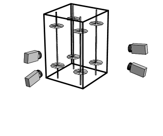
Figure 1: Experimental setup

The data acquisition system consists of four commercial CCD cameras with a maximum frame rate of $50\mathrm{Hz}$ at $1000\times 1000$ pixels. The measurement volume covers roughly $1000\mathrm{cm}^{3}$. We use polystyrene particles with size $\sim 400\mathrm{\mu m}$ and density very close to $1\mathrm{g}/\mathrm{cm}^{3}$. We record $\mathcal{O}(800)$ particles at each time step with an accuracy in the estimation of the particle position of $0.05$ pixels corresponding to a standard deviation $\sigma_{jitter}\sim 10\mathrm{\mu m}.$ The particles are illuminated by a $250\mathrm{W}$ flash lamp.

The Stokes number $St=\tau_{R}/\tau_{\eta}$ measures the ratio between the relaxation time, $\tau_{R}$, of particle motion relative to the fluid and the Kolmogorov time scale, $\tau_{\eta}$. Here $\tau_{R}=(1/18)(\rho_{p}/\rho_{f})(d_{p}^{2}/\nu)$ where $\rho_{f}$ is the density of the fluid and $\rho_{p}$ and $d_{p}$ are the density and the size of the particles respectively. We get $St=0.01$ and thus much less than one. The particles can therefore be treated as passive tracers in the flow.

The mathematical algorithms for translating two dimensional image coordinates from the four camera chips into a full set of three dimensional trajectories in time involve several crucial steps: fitting 2d gaussian profiles to the 2d images, stereo matching (line of sight crossings) with a two media (water-air) optical model and construction of 3d trajectories in time by using a kinematic principle of minimum change in acceleration Willneff (2003); Ouellette et al. (2006a).

If a particle can not be observed from at least three cameras the linking ends. Most of the the time this happens because the particles shade for each other. The higher the seeding density of particles the higher the risk of shadowing. Since the seeding is relatively high we obtain shorter tracks than we would have in the case of only a few particles in the tank. Since the particles most often only disappear from one or two cameras for a few time steps, a new track starts when the particle is again in view from at least three cameras. The track is hence broken into smaller segments. Through kinematic prediction we are able to connect the broken track segments into longer tracks. We use the method of Xu (2008). The result is satisfactory with a substantial increase in the mean length of the tracks.

The flow characteristics are presented in Table 1. With $\tau_{\eta}=0.08\mathrm{s}$ and a recording frequency at $50\mathrm{Hz}$ the temporal resolution is $\sim 4\mathrm{frames}/\tau_{\eta}$. The mean flow is axisymmetric with a significant vertical straining on the largest scales and no significant differences from the flow reported in (Berg et al., 2006; Lüthi et al., 2007), where properties of the mean flow can be found.

We choose a coordinate system centered approximately in the center of the tank where the velocity standard deviation $\sigma_{u}$ has a global minimum. The radial distribution of particles in the measuring volume is presented by the stars in Figure 2. We see that for distances from the center less than $50\mathrm{mm}$, represented by the vertical dashed line, the particles are uniformly distributed. We therefore choose a ball, $B$, with same the center and a radius of $50\mathrm{mm}$, as the volume for all future studies in this paper.

Figure 2: Pdf $p(r)$ of the radial position of particles in the measuring volume ($\star$ symbol). The symbols $\Box$ and $\circ$ represent respectively particles starting and ending a trajectory. The black solid line has a slope equal to two and therefore represent the uniform distribution.

In addition we see that both the start and end position of trajectories are also uniformly distributed within the ball, $B$. This means that tracking failure is independent of position. Trajectories may move in and out of $B$ but only positions inside the sub-volume are considered in the data analysis.

To see whether the particles are statistically independent we check the data against a Poisson distribution. For every tenth frame we place 100 balls of varying radius randomly within the flow and count the number of particles inside. The result is presented in Figure 3. The top figures show two examples; one for particles inside balls of radius $10\mbox{ mm}$ and one where the ball radius is $30\mbox{ mm}$. From the bottom figure we conclude that the particles obey a Poisson statistic within 8% which is a bit better than the PTV experiment presented in Jørgensen et al. (2005). This means that the particles either cluster or repel each other.

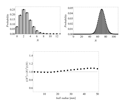
Figure 3: Top: PDF histogram of number of particles within randomly positioned balls of radius $10\mbox{ mm}$ (left) and $30\mbox{ mm}$ (right). The dots represent a Poisson distribution. Bottom: Variation of the ratio $(\langle N^{2}\rangle-\langle N\rangle^{2})/\langle N\rangle$ as function of ball radius. The horizontal line represent the Poisson value of unity.

$\sigma_{u}$	$\varepsilon$	$\eta$	$L$	$\tau_{\eta}$	$T_{E}$	$Re_{\lambda}$
$20.00\mathrm{mm/s}$	$145\mathrm{mm^{2}/s^{3}}$	$0.26\mathrm{mm}$	$55.17\mathrm{mm}$	$0.08\mathrm{s}$	$2.76\mathrm{s}$	136

Table 1: Turbulence characteristics: $\varepsilon$ is the mean kinetic energy dissipation, $\eta\equiv(\nu^{3}/\varepsilon)^{1/4}$ is the Kolmogorov length scale with the kinematic viscosity $\nu=0.89\mathrm{mm}^{2}/\mathrm{s}$ of water. $\tau_{\eta}\equiv(\nu/\varepsilon)^{1/2}$ is the Kolmogorov time scale and $\sigma_{u}^{2}=\frac{1}{3}(\sigma_{u_{x}}^{2}+\sigma_{u_{y}}^{2}+\sigma_{u_{z}}^{2})$ is the standard deviation of velocity. The integral length scale is defined as $L=\sigma_{u}^{3}/\varepsilon$ while $T_{E}$ is the eddy turnover time $T_{E}=L/\sigma_{u}$. The Reynolds number is defined as $Re_{\lambda}=\frac{\lambda\sigma_{u}}{\nu}$ with the Taylor micro scale $\lambda=\sqrt{\frac{15\nu\sigma_{u}^{2}}{\varepsilon}}$

The database of trajectories is compiled from $73$ runs performed under identical conditions. Each run consists of $10000$ consecutive frames. After the recording of a run the system was paused for three minutes before a new run was recorded. We therefore consider the $73$ individual runs to be statistically independent. Throughout the paper error bars will therefore be calculated as statistical standard errors of the mean.

II.2 Binomial filtering

Even though we know the position error $\epsilon_{pos}$ to be very small, we choose to filter the data. We choose a binomial filter which has the convenient property of compact support. Using a binomial filter instead of a conventional Gaussian, does not seem to have a large effect (not shown). The weights $w_{k}$ in a binomial filter of length $N$ is given by

$$w_{k}=2^{1-N}\binom{N-1}{k}\hskip 14.22636ptk=0,1,...,N-1$$ (5)

The width of the filter is $\sigma_{filter}=\Delta t\sqrt{N-1}/2$. We apply the binomial filter on the position measurements treating each dimension separately. The velocity and acceleration are then simply given by finite differences

$$\tilde{v}_{i}(t+\Delta t/2) = \frac{\tilde{x}_{i}(t+\Delta t)-\tilde{x}_{i}(t)}{\Delta t}$$ (6)

$$\tilde{a}_{i}(t) = \frac{\tilde{x}_{i}(t+\Delta t)-2\tilde{x}_{i}(t)+\tilde{x}_{i}(t-\Delta t)}{\Delta t^{2}},$$

where $\tilde{\cdot}$ denotes filtered quantities.

We inspect filters with a length from $N=1$ (unfiltered) to $N=20$ and look at the standard deviation and flatness of velocity and acceleration as functions of the filter standard deviation relative to the Kolmogorov time scale $\tau_{\eta}$. These are displayed in figure 4. While velocity seems to be unaltered by the filtering the acceleration is very dependent on filter length. This is a general problem with measurements of accelerations.

Figure 4: left: $\sigma_{u}$ ($\star$) and $\sigma_{a}$ ($\bullet$) as functions of filter width $\sigma_{filter}$ divided by Kolmogorov time scale $\tau_{\eta}$. right: Flatness $F_{u}$ ($\star$) and $F_{a}$ ($\bullet$). The dotted vertical lines denote a filter of length $N=4$ corresponding to $0.23\tau_{\eta}$.

Both the standard deviation and flatness are functions of the filter width. The amount of filtering is a trade off between eliminating noise and eliminating the real signal. The figure does not give a clear indication of which filter to use. We therefore also look at the acceleration pdf. Since this is the limiting PDF for velocity increments $\delta\mathbf{v}(\tau)$ it might seem important for the outcome of results on Lagrangian structure functions. In figure 5 we show the pdf of acceleration as a function of the filter length.

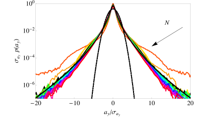
Figure 5: Acceleration pdf $p(a_{y})$ for the component along the axis of forcing in the tank. The pdf is normalized with the standard deviation of acceleration $\sigma_{a_{y}}$ for the same component. The different colors represent the different filter lengths $N$ ranging from $1$ to $20$ following the direction of the arrow. The two black curves are the gaussian distribution and a stretched exponential fitted to the curve for $N=4$ (only partly visible as the thin black curve below the fitted stretched exponential).

From $N=4$ the shape of the pdf becomes more or less constant with $N$. The fat tails of the pdf based on unfiltered data ($N=1$) are likely to be due to noise and perhaps bad connection of tracks. Filtering removes the noisy tails and makes it possible to estimate moments up to $\langle a^{8}\rangle$. The critical filter length for which convergence is achieved is $N=4$. $N=4$ corresponds to a filter width of $0.23\tau_{\eta},$ i.e. well below the Kolmogorov scale. It should be emphasized that choosing $N=4$ is still somewhat arbitrary since there is no rigorous way to determine the optimal filter. Unless otherwise stated $N=4$ has been used in the remainder of the paper.

We have fitted a stretched exponential of the form $p(a)=N_{f}\exp(-a^{2}/((1+|a\beta_{f}/\sigma_{f}|)^{\gamma_{f}})\sigma_{f}^{2})$ to the pdf of scaled acceleration for $N=4$. With $\beta_{f}=0.65,$ $\sigma_{f}=0.55$ and $\gamma_{f}=1.40$ the fit is excellent. The same functional fit for $p(a)$ was used by Porta et al. (2001) with slightly different fit parameters. We can also give an estimate for the dimensionless constant $a_{0}$ in the Heisenberg-Yaglom relation $\langle a_{i}a_{j}\rangle=a_{0}\varepsilon^{3/2}\nu^{-1/2}\delta_{ij}$. In principle $a_{0}$ is not a constant but a function of Reynolds number. It has been well studied in the literature and it is closely connected to Lagrangian stochastic models. Sawford et al. (2003) fits functional forms of $a_{0}$ as function of Reynolds number to data obtained from DNS and high Reynolds number PTV. The values obtained from the PTV data are approximately $30\%$ larger than for the corresponding DNS data. In addition strong anisotropy is observed in the PTV data. We get $a_{0}=4.5\pm 0.3$ for the component averaged acceleration variance while only $a_{0}=3.8\pm 0.2$ for the component along the axis of forcing. For the axial component Sawford et al. (2003) suggest $a_{0}=6.5(1+134Re_{\lambda}^{-1})^{-1}$ giving $a_{0}=3.3$ for the present Reynolds number. The construction of our apparatus does, however, not give us the opportunity to investigate a large span in Reynolds numbers which would be necessary to verify functional forms of $a_{0}$.

As already mentioned the filtering has a large impact on acceleration. Besides that, there is a slight chance that we might underestimate accelerations since variations at the smallest temporal scales simply cannot be resolved. In the PTV data presented in Sawford et al. (2003); Porta et al. (2001) the ratio between $\tau_{\eta}$ and sampling frequency is $\sim 23\mbox{ frames}/\tau_{\eta}$ (for $Re_{\lambda}\sim 870$) compared to only $\sim 4\mbox{ frames}/\tau_{\eta}$ in our experiment. Their data is, however, much noisier, so that their chosen filter width of $\sigma_{filter}/\tau_{\eta}=0.15$ is close to our of $0.23$ for $N=4$.

The motivation behind filtering the trajectories was to eliminate noise, i.e. the error, $\epsilon_{pos}$, associated with determining the position of a particle. Even though $\epsilon_{pos}$ might be both random, unbiased and uncorrelated it still contributes to, for example, the Lagrangian structure functions. To see this we assume that $x_{i}(t)=\hat{x}_{i}(t)+\epsilon_{pos}(t)$. $x_{i}(t)$ is a measured component of position on a trajectory while $\hat{x}_{i}(t)$ is the true position. Furthermore we assume $\langle\epsilon_{pos}(t)\rangle=0$ and $\langle\epsilon_{pos}(t_{1})\epsilon_{pos}(t_{2})\rangle=\sigma_{jitter}^{2}$ if $t_{1}=t_{2}$ and zero otherwise.

The correction to the structure functions is now straight forward to calculate. Since a different number of particle positions are involved in the calculation as a function of time lag, $\tau$, the correction becomes a function of the time lag, $\tau$, itself. With filter $N=4$ we get for the second order measured structure function $S_{2}^{m}(\tau)$

$$S_{2}^{m}(\tau)=S_{2}(\tau)+\sigma^{2}_{error}(\tau)$$ (7)

where $\sigma^{2}_{error}(\tau)$ is given by

$$\sigma^{2}_{error}(\tau)=\begin{cases}\frac{3}{16}\frac{\sigma_{jitter}^{2}}{\Delta t^{2}}&\text{for $\tau=\pm\Delta t$},\\ \frac{7}{16}\frac{\sigma_{jitter}^{2}}{\Delta t^{2}}&\text{for $\tau=\pm 2\Delta t$},\\ \frac{7}{16}\frac{\sigma_{jitter}^{2}}{\Delta t^{2}}&\text{for $\tau=\pm 3\Delta t$},\\ \frac{11}{16}\frac{\sigma_{jitter}^{2}}{\Delta t^{2}}&\text{for $\tau=\pm 4\Delta t$},\\ \frac{5}{16}\frac{\sigma_{jitter}^{2}}{\Delta t^{2}}&\text{for $\tau=\pm n\Delta t,$ $n\geq 5$}.\\ \end{cases}$$ (8)

We find that the correction to the measured higher order structure functions $S_{p}^{m}(\tau)$ is given by

$$S_{p}^{m}(\tau)=S_{p}(\tau)+A_{p}\sigma^{2}_{error}(\tau)S_{p-2}^{m}(\tau),$$ (9)

with $S_{0}=1$ for all time lags $\tau$. We have omitted terms of higher order in $\sigma_{error}$. $A_{p}$ is given by

$$A_{p}=\frac{p^{2}-p}{2}.$$ (10)

With $\sigma_{jitter}\sim 10\mu\mathrm{m}$ the corrections $\sigma^{2}_{error}(\tau)$ are of order $10^{-3}\mathrm{mm}^{2}/\mathrm{s}^{2}$.

III Bias of Lagrangian statistics

A practical property of the present experiment is the stationarity of Eulerian velocity statistics. The Lagrangian statistics are, on the other hand, not stationary in the measurement volume, $B$.

A particle which enters $B$ will loose kinetic energy during its travel inside $B$. This reflects the non-uniform forcing in space in our experiment. On average the particles gain kinetic energy close to the propellers located outside $B$. During their subsequent motion the particles lose kinetic energy until they again come close to the propellers which are constantly spinning. Thus there is a flux of kinetic energy into $B$. Inside the volume the kinetic energy is dissipated and hence we have $\frac{1}{2}\frac{d}{dt}\langle\mathbf{v}^{2}\rangle\sim-\varepsilon$  Ott and Mann (2005). The equation can be derived directly from the Navier-Stokes equation by assuming global homogeneity Mann et al. (1999) which, as already mentioned, is only approximately true for this experiment.

In DNS the random forcing occurs in fourier space and is hence globally homogeneous. We therefore have $d\langle v^{2}\rangle/dt=0$ and consequently Lagrangian stationarity. However, most physical flows encountered in nature, as for example the atmospheric boundary layer, will seen in a finite volume be Lagrangian non-stationary.

Particles with fast velocity tend to leave the measurement volume after only a short amount of time. This means that those particles that stays in the volume for long times often are those with the smallest velocity. The effect is a bias for long times towards slow particles. It should be emphasized that this is a systematic error whereas the Lagrangian non-stationarity is a genuine property of the flow.

Exactly how one should compensate for the systematic error is an open question. In this paper we will build on the ideas first presented by Ott and Mann (2005). Here the Lagrangian structure functions $S_{p}(\tau)$ are expressed through the mean Greens function $G(\mathbf{r},\tau)$ as

$$S_{p}(\tau)=\int_{\mathcal{R}^{3}}S_{p}(\tau|\mathbf{r})G(\mathbf{r},\tau)d^{3}r,$$ (11)

where $S_{p}(\tau|\mathbf{r})$ is the conditional Lagrangian structure function of order $p$ defined as the mean of $|\delta v|^{p}$ conditioned on the distance travelled $\mathbf{r}$ after a time lag $\tau$. The mean Greens function for one-particle diffusion $G(\mathbf{r},\tau)$ is the probability density of getting $\mathbf{r}$ after a time lag $\tau$. The relation is evidently exact. However, when the field of view is limited the integration on the right hand side is truncated which leads to systematic errors. It is truncated by a filter $W(r)$ that expresses the probability that a point $\mathbf{x}_{2}$ separated a distance $r$ from another point $\mathbf{x}_{1}$ lies inside a ball with radius $R$. Here $\mathbf{x}_{1}$ is chosen randomly inside the ball. Assuming homogeneity $W(r)$ is a purely geometric factor of the distance $|\mathbf{x}_{1}-\mathbf{x}_{2}|=r$. It is given by

$$W(r)=\begin{cases}(1-\frac{r}{2R})^{2}(1+\frac{r}{4R})&\text{for $r<2R$},\\ 0&\text{for $r>2R$}.\end{cases}$$ (12)

If we neglect the finite measurement volume and just average the velocity differences that we have actually measured, the experimental structure function becomes

$$S_{p,meas}(\tau)=\frac{\int W(r)S_{p}(\tau|r)4\pi r^{2}G(r,\tau)dr}{\int W(r)4\pi r^{2}G(r,\tau)dr}.$$ (13)

Ott and Mann proposed an improved method where $W(r)$ is removed from eqn. 13: each pair is binned with weight $1/W(r)$. Since $W(2R)=0,$ pairs with separations very close to $2R$ should be disregarded since they would otherwise make the compensation explode. We therefore limit separations to $2R-\delta$. In the present case $2R=100\mathrm{mm}$ and $\delta=5\mathrm{mm}$.

Including compensation we can now write eqn. 13 as

$$S_{p,meas}(\tau)=\frac{\int_{0}^{2R-\delta}S_{p}(\tau|r)4\pi r^{2}G(r,\tau)dr}{\int_{0}^{2R-\delta}4\pi r^{2}G(r,\tau)dr}.$$ (14)

Figure 6: Mean Greens function $G(r,\tau)$ as a function of $r$ at three different time lags $\tau$. Increasing towards the right, time lags are $\tau=\{5,13,35\}\tau_{\eta}$ with (solid lines) and without (dashed lines) compensation through $W(r)$.

We will use this framework to estimate an upper time lag below which Lagrangian structure functions are not biased by the finite measurement volume. To put it simple we need to figure out whether or not $2R-\delta$ is enough to cover the support of the integrands in eqn. 14.

In Fig. 6 we show the mean Greens function $G(r,\tau)$ as a function of $r$. For the small time lag $\tau=5\tau_{\eta}$ the curves almost collapse indicating that finite volume effects are almost vanishing. Increasing $\tau$ to $13\tau_{\eta}$ we see that finite volume effects are significant as the curves no longer collapse. Both curves, however, go to zero for large values of $r$, which means that the integrand in eqn. 14 converges. This means that for this specific time lag we can calculate finite volume unbiased structure functions if we include compensation. For the largest time lag, $\tau=35\tau_{\eta}$ we see that the compensated $G(r,\tau)$ no longer converges. This means that even the compensation fails.

We now assume $G(r,\tau)$ to be Gaussian and self similar, that is $G(r,\tau)=\exp(-(r/\sigma_{x}(\tau))^{2}/2)/(2\pi^{3/2}\sigma_{x}(\tau)^{3})$. Furthermore we assume that $S_{p}(\tau|r)\sim r^{p}$ for large $r$ and large $\tau$. Figure 7 shows log-log plots of $S_{p}(\tau|r)$ for $p=2,4,6,8$. We observe an approximately agreement with $S_{p}(\tau|r)\sim r^{p}$. Ott and Mann (2005) calculated $S_{2}$ for a gaussian displacement process and found that $S_{2}(\tau|r)\sim r^{2}$ for large $r$. The implications for $S_{p}$ is evident: only the slightest deviation from zero in $G(r,\tau)$ for large $r$ will cause the integrand in the numerator of eqn. 14 not to converge. With the made assumptions we can calculate the relative error on $S_{p}$ from the finite volume.

Figure 7: $\log S_{p}(\tau|r)/S_{p}(\tau)$ as a function of $\log r/\sigma_{x}(tau)$ for $\tau\in(15;25)\tau_{\eta}$. The four panels represents $p=2,4,6,8$ with fits $r^{p}$ for large $r/\sigma_{x}(tau)$.

For the compensated structure function the relative error given by $1-S_{p,meas}/S_{p}$. $S_{p,meas}$ can be calculated from eqn. 14 while $S_{p}$ is given by eqn. 11 integrating all the way to infinity. Likewise we can calculate the error without compensation. In this case $S_{p,meas}$ can be calculated from eqn. 13. The results are presented in Figure 8 for $p$=2,4,6 and 8. The solid lines represent the compensated structure functions while the dashed lines represent the uncompensated. The error is a function of the non dimensional variable $\sigma_{x}/R$.

Figure 8: Relative error estimates for $S_{p}$ for $p=2,4,6$ and 8. Dashed lines are without compensation while solid lines are with compensation

It is evident that without compensation we get large, systematic errors even for quite small values of $\sigma_{x}/R$ while the compensation works up to a point where the upper limit of integration ($2R-\delta$) is felt, and the compensation rapidly deteriorates as we move beyond this limit. The upper limit on $\sigma_{x}(\tau)/R$ defines a critical time lag $\tau_{crit}$ where measurements for $\tau>\tau_{crit}$ exhibit a serious, systematic error. For $p=2$ the critical limit is $\sigma_{x}(\tau_{crit})/R\sim 0.5$ while it is $\sigma_{x}(\tau_{crit})/R\sim 0.4$ for $p=8$. Actually these estimates are optimistic because $G$ in practice tends to have fatter tails than a Gaussian. This is shown in Figure 9.

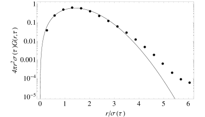
Figure 9: $G(r,\tau)$ for $\tau=10\tau_{\eta}$. The full line is a Gaussian.

In order to get an estimate of $\tau_{crit}$ we set $\sigma_{x}(\tau)\sim\sigma_{u}\tau$ leading to

$$\frac{\tau_{crit,p}}{\tau_{\eta}}\sim C_{p}\,\frac{R}{\sigma_{u}\tau_{\eta}}=15^{-1/2}C_{p}\frac{R}{L}\,R_{\lambda}$$ (15)

with $C_{2}\sim$0.6, $C_{4}\sim$0.53, $C_{6}\sim$0.49 and $C_{8}\sim$0.45 and the integral scale $L=\sigma^{3}/\varepsilon$. $L$ was chosen because it is defined by the geometry of the apparatus used independent of $R_{\lambda}$. From (15) we see that $\tau_{crit}/\tau_{\eta}$ increases with $R_{\lambda}$, thus making it easier to measure at high Reynolds numbers. In other respects, such as the demand on frame speed, it of course gets harder. If we wish to study large time scales, the ratio $\tau_{crit,p}/T_{L}$, where $T_{L}=\sigma^{2}/\varepsilon$ is the Lagrangian integral time scale, could be more relevant and we can note that

$$\frac{\tau_{crit,p}}{T_{L}}=C_{p}\frac{R}{L}.$$ (16)

In other words, finite size effects are not affected by the Reynolds number at large time scales.

Using eqn. 15 with the present data we find $\tau_{crit,2}/\tau_{\eta}=18$, $\tau_{crit,4}/\tau_{\eta}=16$, $\tau_{crit,6}/\tau_{\eta}=14$ and $\tau_{crit,8}/\tau_{\eta}=13$. This is when a 5% error is accepted. Inspection of the data shows that at these values the (compensated) integrands in eqn. 14 are indeed just covered within $2R-\delta$. Without compensation we find very small critical limits: $\tau_{crit,2}/\tau_{\eta}=3.3$, $\tau_{crit,4}/\tau_{\eta}=2.0$, $\tau_{crit,6}/\tau_{\eta}=1.6$ and $\tau_{crit,8}/\tau_{\eta}=1.2$.

Other studies have also looked at the bias effect of Lagrangian statistics Mordant et al. (2004); Biferale et al. (2008); Jørgensen et al. (2005). The criterion in eqn. 15 and eqn. 16 are the strictest yet presented in the literature. The most important lesson is, however, not the limits suggested by the equations themselves, but the compensation: without this, even small time lag statistics are heavily biased as seen in Figure 8.

IV Inertial range scaling

IV.1 Presentation of data

The linear dependence of $Re_{\lambda}$ on $T_{L}/\tau_{\eta}$ implies that a very high Reynolds number is needed in order to obtain a clear Lagrangian inertial range. Yeung (2002) concluded, based on extrapolations from Eulerian fields in DNS, that at least $Re_{\lambda}\sim 600-700$ is needed. Experimental flows at $Re_{\lambda}=1000$ Mordant et al. (2004) and $Re_{\lambda}=815$ Ouellette et al. (2006b) do, however, not show a very pronounced range with a linear regime in the second-order structure function, $S_{2}(\tau)=C_{0}\varepsilon\tau$, and one could speculate if such a range exists at all. $C_{0}$ plays a crucial role in stochastic models (Sawford, 2001) and has been shown to reflect anisotropy in the large-scale forcing (Ouellette et al., 2006b). In Figure 10 we present results of $C_{0}$ for the isotropic ensemble as well as for the three directions.

Figure 10: $C_{0}:$ The circles represent the two horizontal directions while the squares represents the axial direction. The stars are the mean (eqn. I). The arrow indicates the maximum $C_{0}=4.46$ at $\tau=2.96\tau_{\eta}$.

According to $S_{2}(\tau)$, $C_{0}$ should be determined from a plateau in the inertial range. The inertial range is almost vanishing in our experiment. The $\star$ symbols are calculated from eqn. I. The maximum is $C_{0}=4.46$ at a time lag $\tau/\tau_{\eta}=2.96$ and therefore mainly associated with small scales. The $\circ$ symbols represent the horizontal directions ($C_{0}=4.88$ and $C_{0}=4.69$) while the $\Box$ symbols represent the axial direction ($C_{0}=3.83$). A rough estimate of the error on $C_{0}$ is $0.3$, originating from a $10\%$ error in the determination of the kinetic energy dissipation $\varepsilon$. The statistical error is essentially zero.

It is interesting to see that the slight anisotropy in the forcing is manifested all the way down to $\tau\sim\tau_{\eta}$. The propellers forcing the flow are attached to four rods placed in the corners of the tank. The reason for the horizontal components being different is probably small differences in the vertical placement of the propellers on the rods. The lack of small-scale isotropy in the current experiment should not necessarily be taken as a failure of Kolmogorov’s hypothesis of local isotropy. For such a statement the Reynolds number in our experiment is simply not high enough. Other experiments at much higher Reynolds number do, however, all indicate that the large scale inhomogeneities are also present at smaller scales although with smaller amplitude Shen and Warhaft (2000, 2002); Ouellette et al. (2006b). These findings are striking and may suggest that the hypothesis of local isotropy and the concept of locality should be reviewed Tsinober (2001).

A theory that demands isotropy, as is the case of most K41-like predictions can literarily not be falsified, since the perfect experiment with isotropic forcing and hence isotropy on the smallest scales can not be constructed. This was one of the motivations behind the construction of the isotropic ensemble given in eqn. I.

Alternatively one can calculate $C_{0}$ from the velocity spectrum. Arguments put forward by Lien and D’Asaro (2002) state the inertial range scaling is easier to obtain in Fourier space through the velocity spectrum. However, no difference was observed in the present data set through such an analysis (not shown).

We now look at the higher order structure functions. We want to quantify the degree of intermittency through anomalous scaling exponents. The structure functions $S_{p}(\tau)$ for $p=2,4,6,8$ are displayed in Figure 11. It should be remembered that the data are heavily influenced by finite volume bias for time lags $\tau\geq\tau_{crit}$. The most important conclusion to state from the plot is the evident lack of power law behavior and hence a $K41$ scaling regime.

Figure 11: Lagrangian structure functions $S_{p}(\tau)$ as a function of time lag $\tau$. $p$ is increasing upwards with $p=2,4,6,8$. The different structure functions have been shifted vertically for clarity.

Motivated by the lack of a clear inertial range in accessible turbulent data, Benzi et al. (1993) introduced Extended Self Similarity (ESS). Even though it was originally applied to Eulerian data it in can easily be adapted to Lagrangian. Instead of plotting $S_{p}(\tau)$ against time lag $\tau$, $S_{p}(\tau)$ is plotted against the structure function not affected by intermittency for the corresponding time lag.

In more general terms we define in the ESS context the anomalous scaling exponents $\zeta_{p}(\tau)$ through

$$\zeta_{p}(\tau)=\frac{d\log{[S_{p}(\tau)]}}{d\log{[S_{2}(\tau)]}}.$$ (17)

It has obvious advantages compared to conventional ad hoc power law fitting procedures Arnèodo et al. (2008). It can, however, be difficult to quantify from experimental data due to the derivative which is very sensitive to noise.

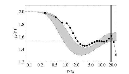
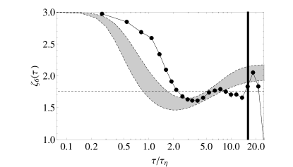
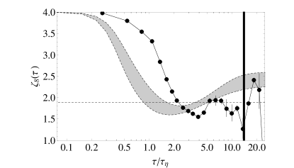
Figure 12: $\zeta_{p}(\tau)$. Top: $p=4$, middle: $p=6$ and bottom: $p=8$ (solid curves). The shaded areas represent the the multifractal predictions: the upper boundary is based on longitudinal Eulerian structure functions while the lower boundary is based on transverse Eulerian structure functions. The thick black vertical lines denote the critical time lags according to Section III. We find the large time lag saturation levels to be $1.53,1.76,1.93$ for $p=4,6,8$. The error bars refer to statistical errors.

$\zeta_{p}(\tau)$ for $p=4,6,8$ are plotted in Figure 12. Two general trends are observed in all three figures.

A dip around $2\tau_{\eta}\leq\tau\leq 5\tau_{\eta}$ is observed. Hereafter a plateau is reached. For increasing order $p$ the dip becomes larger and $\zeta_{p}$ saturates at a higher level in agreement with the findings and speculations by Arnèodo et al. (2008). The saturation levels are displayed with horizontal lines at $1.53$, $1.76$ and $1.93$ respectively. At time lags around $\tau_{crit}$ we see that the error bars grow significantly at least for $p=8$. With increasing $p$ it even happens before $\tau_{crit}$ as also suggested in Section III and makes a plateau hard to observe.

The dip has been associated with vortex trapping Biferale et al. (2005) where particles are trapped in strong vortices with time scale close to $\tau_{\eta}$. An example of such a particle is displayed in Fig. 13. At around $t\sim 50\tau_{\eta}$ the particle experiences extreme accelerations (around $10$ times the rms value) and seems to be caught in a vortex-like structure.

We thus support the findings already reported in Biferale et al. (2005); Porta et al. (2001) in studies of much more vivid flow. However, we demonstrate that the value of the Reynolds number is not necessarily crucial in order to observe characteristic turbulence features in the Lagrangian frame as is also known from low Reynolds number DNS. Differences in DNS and physical flows are, however, notable and careful analysis of both is therefore important in order to obtain a complete picture.

It is also striking that the maximum of $S_{2}(\tau)/\tau$ is at $\tau=2.96\tau_{\eta}$ which is very close to the position of the viscous dip of $\zeta_{4}(\tau)$. Whether this has any significance is not at all clear. If so, it is a challenge for stochastic models, which do not take the viscous dip into account.

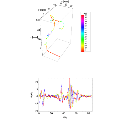
Figure 13: Top Sample particle. The color denotes the magnitude of the acceleration. Bottom Particle acceleration in units of the standard deviation $\sigma_{a}$ for all three components.

IV.2 Multifractal model

In Fig. 12 we have also plotted the multifractal prediction. The multifractal model is developed in the Eulerian frame by Parisi and Frisch (1983) to characterize the spatial structure of dissipation in turbulence it was later adapted in the Lagrangian frame by Borgas (1993). It gives a translation between the two frames and as such works as a bridge between them. Work presented in Biferale et al. (2004, 2005); Chevillard et al. (2003); Mordant et al. (2002, 2004); Xu et al. (2006b) has shed light on the issue of multifractals in the Lagrangian frame through a number of high Reynolds number experiments and DNS which were well captured by the theory through ESS scaling relationships for time lags $\tau\geq\tau_{\eta}$. With the extension by Chevillard et al. (2003) the multifractal framework is now capable of taking into account also the vortex trapping behavior taking place at time lags $\tau\sim\tau_{\eta}$.

In Arnèodo et al. (2008) it was shown for $\zeta_{4}(\tau)$ how the multifractal model matches results from experimental and numerical data on all time scales independently of Reynolds number. The data set used in this paper is the one denoted EXP 1 in that paper. Here we show that for $p=6$ and $p=8$ the multifractal model seems somewhat less perfect.

In the multifractal model the flow is assumed to possess a range of scaling exponents $h_{min},...,h_{max}$ with a certain probability so that the velocity difference by separation $r$ is $\delta_{r}u\sim r^{h}$. For each scaling exponent $h$ there is a fractal set with a $h$-dependent dimension $D(h)$. The embedding dimension is three $(r\in\mathcal{R}^{3})$ and hence $D(h)\leq 3$ for all $h$. The probability $P_{h}(r)$ of having an exponent $h$ at separation $r$ is therefore proportional to $3-D(h)$. From dimensional arguments the Eulerian velocity fluctuation $\delta_{r}u$ is related to a Lagrangian time lag $\tau$. That is $\tau\sim r/\delta_{r}u$. Recently focus on this relation has cast serious doubt on its usage Homann et al. (2007); Yakhot (2008); Kamps et al. (2008). In Kamps et al. (2008) it is shown how the relation $\tau\sim r/\delta_{r}u$ is the limiting case of something more general. In three dimensional turbulence they show that Lagrangian statistics is much more influenced by Eulerian integral and dissipation scales than the simple picture suggest, where the time lag $\tau$ is only associated with eddies of size $r$. This is also what we already know from Figure 6 and from eqn. 11 where contributions from all scales is included in the integral. The conclusion must be that good statistics of all Eulerian scales are necessary in order to calculate Lagrangian structure function - even at small time lags. At present DNS does not resolve the statistics of the largest scales sufficiently. PTV experiments do not have this problem.

Following Arnèodo et al. (2008) closely we can calculate the multifractal prediction for $p=4,6,8$. We choose the same model constants and functional form of $D(h)$ as in Arnèodo et al. (2008) since these were shown to fit a large number of experiments and DNS simulations for $p=4$.

We again take a look at Figure 12. The result in Arnèodo et al. (2008) ($p=4$) is reproduced: Following the multifractal longitudinal curve (upper) in the dip quite close, $\zeta_{4}(\tau)$ saturates at a value close to the multifractal transverse curve (lower). For $p=6$ and $p=8$ the multifractal predicted curves does not fit the data. First, the plateau in the data does not reach the level of the multifractal prediction before finite volume bias effects become important. This bias has the effect of lowering the value of $\zeta_{p}(\tau)$. Second, for both moments the dip is shifted towards the left. The dip minimum does, however, seem to match the data. In the multifractal model there is a free parameter included in the model definition of the dissipative time scale. We have set this constant, $t_{scale}$ equal to $7$. Its only job is to scale the $\tau/\tau_{\eta}$ axis. The same constant value was used in Arnèodo et al. (2008) in order to fit the model prediction to data for $p=4$. Since $t_{scale}$ must be independent of $p$, we could equally well have fitted $t_{scale}$ to the data for $p=6$ or $p=8$. If we had done so we would encounter a bad match for $p=4$ and $p=8$ or $p=4$ and $p=6$ respectively.

Why the multifractal model fail to predict the different moments of $\zeta_{p}(\tau)$ is a relevant question. We could speculate that the temporal resolution in our experiment is not high enough to resolve the smallest scale. In order to investigate this we look at the importance of filtering. We picture the increase of filter length as a way of decreasing the temporal resolution and calculate $\zeta_{p}(\tau))$ as a function of filter length, $N$. For $N\leq 10$ the resuls are presented in Figure 14.

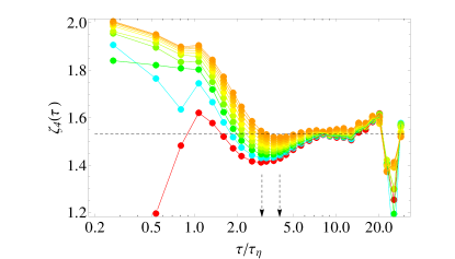
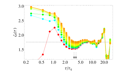
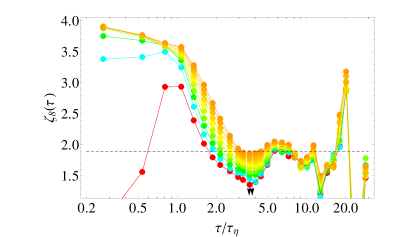
Figure 14: $\zeta_{p}(\tau)$. Top: $p=4$, middle: $p=6$ and bottom: $p=8$ (solid curves). The colors denote different filter $N$ (increasing upwards from $N=1$ (red)). Arrows indicate minimum position for $N=1$ (left arrow) and $N=10$ (right arrow).

With increasing filter length we see that the dip region is depleted and the position of the minimum on the $\tau$ axis is shifted to the right (the arrows indicate the position of the local minimum for $N=1$ and $N=10$). The shift in position is decreasing with increasing $p$ and hardly observable for $p=8$. The saturation level is more or less constant with $N$. Both the quantitative and qualitative shape of the dip region of $\zeta_{p}(\tau)$ are therefore quite sensitive to the filter length $N$. How does this relate to the multifractal model? In Figure 12 we see that the dip position of the multifractal model is almost constant with $p$, while the data show a shift towards smaller time lags when $p$ is increased. On the other hand, we observe in Figure 14 that for $p=4$ the shift is towards larger time lags whereas it is almost non-existing for $p=8$. That is, for a higher resolution, here pictured as a lower filter, the multifractal model would work even worse.

V Discussion and conclusions

Analyzing Lagrangian data uncritically can lead to substantial biases. Building on the ideas first presented by Ott and Mann (2005) we have found a robust way to compensate for the finite volume bias. We show that the time lags for which finite volume bias can be neglected are limited. We also saw that the finite volume effects increase for increasing order $p$ of the structure functions. Observing extreme statistics might therefore be very difficult. We are convinced that the present study and its consequences should be kept in mind when designing future experiments for measuring Lagrangian statistics: in a high Reynolds number flow the separation between the integral scale and the Kolmogorov length is very large. In order to follow particles and measure the Lagrangian structure functions for large time lags without finite volume bias the camera chip needs to be extremely big, which is currently a technical obstacle. Alternative setups where different camera systems focus on the small and the large scales simultaneous could be the solution to this problem. DNS does not suffer from finite volume bias. On the other hand DNS may still have problems with small time lags due to interpolation from the Eulerian flow field Biferale et al. (2008).

In particular we have studied one-particle statistics in terms of Lagrangian structure functions. We have looked at the small time scale behavior which seems to be affected by the large-scale inhomogeneities present in our flow. This led us to work with isotropic ensembles. In this way we can test our data against theories developed in an isotropic frame such as the multifractal model.

We do not observe any signs of an inertial range and K41 scaling but by Extended Self-Similarity we are able to extract a quantitative measure of the structure functions of high order. From the local slopes of these we calculate the Lagrangian anomalous scaling exponents and find excellent agreement with already published results.

Measured local slopes of the Lagrangian structure functions are quite similar to results obtained with the multifractal model for $p=4$. With the assumptions and physical reasoning leading to the development of the multifractal model in mind, this is actually a bit surprising. Many of the crucial assumptions behind the multifractal model in the Lagrangian frame are not fulfilled. First of all the multifractal model is motivated by the invariance of the Navier-Stokes equation to an infinite number of scaling groups in the limit of infinite Reynolds number far from present in our data. Second, an exact result such as the 4/5 law does not exist in the Lagrangian frame. The phenomenological picture of the multifractal model with the flow region consisting of active and inactive regions in direct contrast to the Richardson picture where eddies are space filling does, however, fit observed flow features such as a dip region in $\zeta_{p}(\tau)$ and anomalous scaling.

For $\zeta_{6}(\tau)$ and $\zeta_{8}(\tau)$ the situation is different. The multifractal model fails to describe the data: although the qualitative behavior is similar to $\zeta_{4}(\tau)$ the shift in dip position as a function of $p$ is much more pronounced in our data than in the multifractal model. We are curious to see results from other experiments and DNS simulations for $p>4$. The simple bridging relation, where a time lag is solely associated to the time scale, $\tau$ for the local eddy of size $r$, assumed in the multifractal model might be too crude. Also the filtering was shown to have an effect on the dip region: the strength for all orders of $p$ while the position was only dependent on filtering up to $p=6$. Since almost all data sets, both from physical experiments and from DNS, are noisy and hence must be filtered, conclusions on $\zeta_{p}(\tau)$ should therefore be made with great care.