Perfect simulation of spatial point processes
using dominated coupling from the past with
application to a multiscale area-interaction
point process

Abstract

We consider perfect simulation algorithms for locally stable point processes based on dominated coupling from the past. A version of the algorithm is developed which is feasible for processes which are neither purely attractive nor purely repulsive. Such processes include multiscale area-interaction processes, which are capable of modelling point patterns whose clustering structure varies across scales. We prove correctness of the algorithm and existence of these processes. An application to the redwood seedlings data is discussed.

1 Introduction

One of the long standing problems in Markov chain Monte Carlo is that it is rarely possible to know when the Markov chain we are using for simulation has reached equilibrium. For certain classes of problem, this problem was solved by the introduction of coupling from the past (CFTP) [16, 17]. More recently, methods based on CFTP have been developed for perfect simulation of spatial point process models (see for example [13, 12, 10, 14]).

Exact CFTP methods are therefore attractive, as one does not need to rigorously check convergence or worry about burn-in, or use complicated methods to find appropriate standard errors for Monte Carlo estimates based on correlated samples. Independent and identically distributed samples are now available, so estimation reduces to the simplest case. Unfortunately, this simplicity comes at a price. These methods are notorious for taking a long time to return just one exact sample and are often difficult to code, leading many to give up and return to nonexact methods.

In response to these issues, in the first part of this paper we present a dominated CFTP algorithm for the simulation of locally stable point processes which potentially requires far fewer evaluations per iteration than the existing method in the literature [14].

It is often the case that advancements in statistical theory are inspired by applications, and this is no exception. There are several classes of model for stochastic point processes, for example simple Poisson processes, cluster processes such as Cox processes, and processes defined as the stationary distribution of Markov point processes, such as Strauss processes [19] and area-interaction processes [3].

All of the above mentioned point process models are capable of modelling either clustered or regular point patterns. They are not, however, well suited to modelling point patterns whose clustering structure varies across scales, for example clusters of regularly spaced points or regularly spaced clusters of points. In the second part of the paper we introduce a new multiscale area-interaction process which is capable of modelling either of these types of point pattern. We then demonstrate how the algorithm developed in the first part of the paper may be used to generate samples from this process.

The structure of this papers is as follows. In Section 2 we discuss perfect simulation, beginning with ordinary coupling from the past (CFTP) and moving on to dominated CFTP for spatial point processes. We then introduce and justify our perfect simulation algorithm. In Section 3 we first review the standard area-interaction process. We then introduce our multiscale process, describe how to use our new perfect simulation algorithm to simulate from it, and discuss a method for inferring the parameter values from data. An application to the Redwood seedlings data is presented in Section 4, and some areas for future work are discussed in Section 5.

2 Perfect simulation

2.1 Coupling from the past

The principle behind CFTP is the following. Suppose that it is desirable to sample from the stationary distribution of an ergodic Markov chain $\{Z_{t}\}$ on some (finite) state space $X$ with states $1,\ldots,n$. It is clear that if it were possible to go back an infinite amount in time, start the chain running (in state $Z_{-\infty}$) and then return to the present, the chain would (with probability 1) be in its stationary distribution when one returned to the present (i.e. $Z_{0}\sim\pi$, where $\pi$ is the stationary distribution of the chain).

Suppose now that we were to set not one, but $n$ chains $\{Z^{(1)}_{t}\},\ldots,\{Z^{(n)}_{t}\}$ running at a fixed time $-M$ in the past, where $Z^{(i)}_{-M}=i$ for each chain $\{Z^{(i)}_{t}\}$. Now let all the chains be coupled so that if $Z^{(i)}_{s}=Z^{(j)}_{s}$ at any time $s$ then $Z^{(i)}_{t}=Z^{(j)}_{t}\hskip 10.00002pt\forall t\geq s$. Then if all the chains ended up in the same state $j$ at time zero (i.e. $Z^{(i)}_{0}=j\hskip 10.00002pt\forall i\in X$), we would know that whichever state the chain passing from time minus infinity to zero was in at time $-M$, the chain would end up in state $j$ at time zero. Thus $j$ must be a sample from the stationary distribution of the Markov chain in question.

When performing CFTP, a useful property of the coupling chosen is that it be stochastically monotone as in the following definition.

Definition 1

Let $\{Z^{(i)}_{t}\}$ and $\{Z^{(j)}_{t}\}$ be two Markov chains obeying the same transition kernel. Then a coupling of these Markov chains is stochastically monotone with respect to a partial ordering $\leq$ if whenever $Z^{(i)}_{t}\leq Z^{(j)}_{t}$, then $Z^{(i)}_{t+k}\leq Z^{(j)}_{t+k}$ for all positive $k$.

Whenever the coupling used is stochastically monotone and there are maximal and minimal elements with respect to $\leq$ then we need only simulate chains which start in the top and bottom states, since chains starting in all other states are sandwiched by these two. This is an important ingredient of the dominated coupling from the past algorithm introduced in the next section.

Although attempts have been made to generalise CFTP to continuous state spaces (notably [15] and [9], as well as [14], discussed in Section 2.2), there is still much work to be done before exact sampling becomes universally, or even generally applicable. For example, there are no truly general methods for processes in high, or even moderate, dimensions.

2.2 Dominated coupling from the past

Dominated coupling from the past was introduced as an extension of coupling from the past which allowed the simulation of the area-interaction process [13], though it was soon extended to other types of point processes and more general spaces [14]. We give the formulation for locally stable point processes.

Suppose that we wish to obtain a sample of a spatial point process with density $f$ with respect to the unit rate Poisson process, whose Papangelou conditional intensity, $\lambda_{f}(u;X)$, is uniformly bounded above by some constant $\lambda$:

$$\lambda_{f}(u;X)=\frac{f(X\cup\{u\})}{f(X)}\leq\lambda.$$

The uniform bound on the Papangelou conditional intensity is required in order for the point process to be locally stable, so this is not imposing any additional constraint.

Then the algorithm given in [14] is as follows.

1. Obtain a sample of the Poisson process with rate $\lambda$.

2. Evolve a Markov process $D(T)$ backwards until some fixed time $-T$, using a birth-and-death process with death rate equal to 1 and birth rate equal to $\lambda$. The configuration generated in step 1 is used as the initial state.

3. Mark all of the points in the process with U[0,1] marks. We refer to the mark of point $x$ as $P(x)$.

4. Recursively define upper and lower processes, $U$ and $L$ as follows. The initial configurations at time $-T$ for the processes are

   $$U_{-T}(-T) = \left\{x\;:x\in D(-T)\right\}$$

   $$L_{-T}(-T) = \left\{\boldsymbol{0}\right\}$$

5. Evolve the processes forwards in time to $t=0$ in the following way.

   Suppose that the processes have been generated up a given time, $u$, and suppose that the next birth or death to occur after that time happens at time $t_{i}$. If a birth happens next then we accept the birth of the point $x$ in $U_{-T}$ or $L_{-T}$ if the point’s mark, $P(x)$, is less than

   $$\min\left\{\frac{\lambda_{f}(x;X)}{\lambda}:L_{-T}(t_{i})\subseteq X\subseteq U_{-T}(t_{i})\right\}$$ or (1)

   $$\max\left\{\frac{\lambda_{f}(x;X)}{\lambda}:L_{-T}(t_{i})\subseteq X\subseteq U_{-T}(t_{i})\right\}$$

   respectively, where $x$ is the point to be born.

   If, however, a death happens next then if the event is present in either of our processes we remove the dying event, setting $U_{-T}(t_{i})=U_{-T}(u)\setminus\{x\}$ and $L_{-T}(t_{i})=L_{-T}(u)\setminus\{x\}$.

6. Define $U_{-T}(u+\varepsilon)=U_{-T}(u)$ and $L_{-T}(u+\varepsilon)=L_{-T}(u)$ for $u<u+\varepsilon<t_{i}$.

7. If $U_{-T}$ and $L_{-T}$ are identical at time zero (i.e. if $U_{-T}(0)=L_{-T}(0)$), then we have the required sample from the area-interaction process with rate parameter $\lambda$ and attraction parameter $\gamma$. If not, go to step 2 and repeat, extending the underlying Poisson process back to $-(T+S)$ and generating additional $U[0,1]$ marks (keeping the ones already generated).

This algorithm involves calculation of $\lambda(u;X)$ for each configuration that is both a subset of $U(T)$ and a superset of $L(T)$. Since calculation of $\lambda(u;X)$ is typically expensive, this calculation may be very costly. The method proposed in Section 2.3 uses an alternative version of step 5 which only requires us to calculate $\lambda(u;X)$ for upper and lower processes.

The more general form given in [14] may be obtained from the above algorithm by replacing the evolving Poisson process $D(T)$ with a general dominating process on a partially ordered space $(\Omega,\preceq)$ with a unique minimal element $\boldsymbol{0}$. The partial ordering in the above algorithm is that induced by the subset relation $\subseteq$. Step 5 is replaced by any step which preserves the sandwiching relations

$$L_{-T}(u)\preceq X_{-T}(u)\preceq U_{-T}(u)\preceq D(u)$$ and (2)

$$L_{-T}(t)=U_{-T}(t)\;\text{ if }\;L_{-T}(s)=U_{-T}(s)$$ (3)

for $s\leq t\leq 0$, and the funnelling property

$$L_{-T}(u)\preceq L_{-(T+S)}(u)\preceq U_{-(T+S)}(u)\preceq U_{-T}(u)$$ (4)

for all $u<0$ and $T,S>0$. In equation (2), $X_{-T}(u)$ is the Markov chain or process from whose stationary distribution we wish to sample.

2.3 A new perfect simulation algorithm

Suppose that we wish to sample from a locally stable point process with density

$$p(X)=\alpha\prod_{i=1}^{m}f_{i}(X),$$ (5)

where $\alpha\in(0,\infty)$ and $f_{i}:\mathfrak{R}^{f}\to\mathbb{R}$ are positive valued functions which are monotonic with respect to the partial ordering $\preceq$ induced by the subset relation and have uniformly bounded Papangelou conditional intensity:

$$\lambda_{f_{i}}(u;\mathbf{x})=\frac{f_{i}(\mathbf{x}\cup\{u\})}{f_{i}(\mathbf{x})}\leq K.$$

Then clearly

$$\lambda_{p}(u;\mathbf{x})\leq\lambda=\prod_{i=1}^{m}\max_{X,\{x\}}\lambda_{f_{i}}(x;X)$$ (6)

for all $u$ and $\mathbf{x}$, and $\lambda$ is finite. Thus we may use the algorithm in Section 2.2 to simulate from this process using a Poisson process with rate $\lambda$ as the dominating process.

However, as previously mentioned, calculation of $\lambda_{p}(u;\mathbf{x})$ is typically expensive, increasing at least linearly in $n(\mathbf{x})$. Thus to calculate the expressions in display (1), we must in general perform $2^{n(U_{-T}(t_{i}))-n(L_{-T}(t_{i}))}$ of these calculations, making the algorithm non-polynomial. In practice it is clearly not feasible to use this algorithm in all but the most trivial of cases, so we must look for some way to reduce the computational burden in step 5 of the algorithm.

This can be done by replacing step 5 with the following alternative.

1. Evolve the processes forwards in time to $t=0$ in the following way.

   Suppose that the processes have been generated up a given time, $u$, and suppose that the next birth or death to occur after that time happens at time $t_{i}$. If a birth happens next then we accept the birth of the point $x$ in $U_{-T}$ or $L_{-T}$ if the point’s mark, $P(x)$, is less than

   $$\prod_{i=1}^{m}\left[\max\left\{\lambda_{f_{i}}(u;U(T)),\lambda_{f_{i}}(u;L(T))\right\}\left/\lambda\right.\right]$$ or (7)

   $$\prod_{i=1}^{m}\left[\min\left\{\lambda_{f_{i}}(u;U(T)),\lambda_{f_{i}}(u;L(T))\right\}\left/\lambda\right.\right]$$ (8)

   respectively, where $x$ is the point to be born.

   If, however, a death happens next then if the event is present in either of our processes we remove the dying event, setting $U_{-T}(t_{i})=U_{-T}(u)\setminus\{x\}$ and $L_{-T}(t_{i})=L_{-T}(u)\setminus\{x\}$.

Lemma 1

Step 5’ obeys properties (2), (3) and (4) and is thus a valid dominated coupling from the past algorithm.

Proof Property (2) follows by noting that

$$(\ref{gen-low})\leq\lambda_{p}(u;X)\leq(\ref{gen-up})\leq 1.$$

Property (3) is trivial. Property (4) follows from the monotonicity of the $f_{i}$’s. $\Box$ $\Box$

Theorem 1

Suppose that we wish to simulate from a locally stable point process whose density $p(X)$ with respect to the unit rate Poisson process is representable in form (5). Then by replacing Step 5 by Step 5’ it is possible to bound the necessary number of calculations of $\lambda_{p}(u;X)$ per iteration in the dominated coupling from the past algorithm independently of $n(X)$.

Proof Step 5’ clearly involves only a constant number of calculations, so by Lemma 1 above and Theorem 2.1 of [14] the result holds. $\Box$ $\Box$

In the case where it is possible to write $p(X)$ in form (5) with $m=1$, Step 5’ is identical to Step 5. This is the case for models which are either purely attractive or purely repulsive, such as the standard area-interaction process discussed in Section 3.1. It is not the case for the multiscale process discussed in Section 3.2, or the model studied in [1].

The proof of Theorem 2.1 in [14] does not require that the initial configuration of $L_{-T}$ be the minimal element $\mathbf{0}$, only that it be constructed in such a way as properties (2), (3) and (4) are satisfied. Thus we may refine our method further by modifying step 4 so that the initial configuration of $L_{-T}$ is given by

$$L_{-T}(-T)=\left\{x\in D(-T):P(x)\leq\prod_{i=1}^{m}\left[\min_{X,\{x\}}\lambda_{f_{i}}(x;X)\left/\lambda\right.\right]\right\},$$ (9)

which clearly satisfies the necessary requirements.

3 Area-interaction processes

3.1 Standard area-interaction process

In the standard case, the area-interaction process has density

$$p(X)=\alpha\lambda^{N(X)}\gamma^{-m(X\oplus G)}$$ (10)

with respect to the unit rate Poisson process, where $\alpha$ is a normalising constant, $\lambda>0$ is the rate parameter, $N(X)$ is the number of points in the configuration $X$, $\gamma>0$ is the clustering parameter, $G$ is some compact set in $\mathbb{R}^{d}$ and $X\oplus G$ is Minkowski addition:

$$X\oplus G=\{a\in\mathbb{R}^{d}\mathrel{:}a=x+z\text{, where }x\in X\text{ and }z\in G\}.$$

Here $0<\gamma<1$ is the repulsive case, while $\gamma>1$ is the attractive case. The case $\gamma=1$ reduces the a homogeneous Poisson process with rate $\lambda$.

Figure 1 gives an example of the construction when $G$ is a disc.

Figure 1: An example of some events together with circular “grains” $G$. The events in the above diagram would be the actual members of the process. The circles around them are to show what the set $X\oplus G$ would look like. If $\gamma$ were large, the point configuration on the right would be favoured, whereas if $\gamma$ were small, the configuration on the the left would be favoured.

3.2 A multiscale area-interaction process

The area-interaction process is a flexible model which allows for a good range of models, from regular through total spatial randomness to clustered. Unfortunately it does not allow for models whose behaviour changes at different resolutions, for example repulsion at small distances and attraction at large distances. Some real-world examples of places where we see this sort of behaviour are the distribution of trees on a hillside, or the distribution of zebra in a patch of savannah. A physical example of large scale attraction and small scale repulsion is the interaction between the strong nuclear force and the electro-magnetic force between two oppositely charged particles. The physical laws governing this behaviour are different from those governing the behaviour of the area-interaction class of models, though they may be sufficiently similar so as to provide a useful approximation.

We propose the following model to capture these types of behaviour.

Definition 2

The multiscale area-interaction process has density

$$p(X)=\alpha\lambda^{N(X)}\gamma_{1}^{-m(X\oplus G_{1})}\gamma_{2}^{-m(X\oplus G_{2})},$$ (11)

where $\alpha$, $\lambda$ and $N(X)$, are as in equation (10); $\gamma_{1}\in[1,\infty)$ and $\gamma_{2}\in(0,1]$; and $G_{1}$ and $G_{2}$ are balls of radius $r_{1}$ and $r_{2}$ respectively.

The process is clearly Markov of range $\max\{r_{1},r_{2}\}$. If $G_{1}\supset G_{2}$, we will have small scale repulsion and large scale attraction. If $G_{1}\subset G_{2}$, we will have small scale attraction and large scale repulsion.

Theorem 2

The density (11) is both measurable and integrable.

This is a straightforward extension of the proof of Baddeley and van Lieshout [3] for the standard area-interaction process. For completeness, it is given in Appendix A.

3.3 Perfect simulation of the multiscale process

Perfect simulation of the multiscale process (11) is possible using the method introduced in Section 2.3. Since (11) is already written as a product of three monotonic functions with uniformly bounded Papangelou conditional intensities, we need only substitute into equations (6–9) as follows.

Substituting into equation (6), we find that the rate of a suitable dominating process is

$$\lambda\gamma_{2}^{-m(G_{2})}.$$

The initial configurations of the upper and lower process $U$ and $L$ are then found by simulating this process, thinning with a probability of

$$\gamma_{1}^{-m(G_{1})}\gamma_{2}^{m(G_{2})}$$

for $L$.

As $U$ and $L$ evolve towards time $0$, we accept points $x$ in $U$ with probability

$$\gamma_{1}^{-m((x\oplus G_{1})\setminus U_{-T}(u)\oplus G_{1})}\gamma_{2}^{m(G_{2})-m((x\oplus G_{2})\setminus L_{-T}(u)\oplus G_{2})}$$ (12)

and accept events in $L$ whenever

$$P(x)\leq\gamma_{1}^{-m((x\oplus G_{1})\setminus L_{-T}(u)\oplus G_{1})}\gamma_{2}^{m(G_{2})-m((x\oplus G_{2})\setminus U_{-T}(u)\oplus G_{2})}.$$ (13)

Figure 2 gives examples of the construction $(x\oplus G)\setminus Y_{-T}(u)\oplus G$.

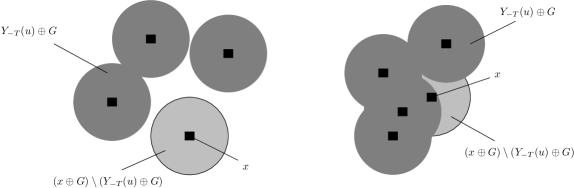
Figure 2: Another look at Figure 1 with some shading added to show the process of simulation. Dark shading shows $Y_{-T}(u)\oplus G$ where $Y_{-T}(u)$ is the state of either $U$ or $L$ immediately before we add the new event and $G$ could be either $G_{1}$ or $G_{2}$. Light shading shows the amount added if we accept the new event. In the configuration on the left, $x\oplus G=(x\oplus G)\setminus(Y_{-T}(u)\oplus G)$, so that the attractive term in (12) or (13) will be very small, whereas the repulsive term will be large. In the configuration on the right we are adding very little area to $(Y_{-T}(u)\oplus G)$ by adding the event, so the attractive term will be larger and the repulsive term will be smaller.

3.4 Parametric inference

We use maximum pseudo-likelihood [5, 6, 7, 11] to estimate the parameters $\lambda$, $\gamma_{1}$ and $\gamma_{2}$.

As we saw in Section 3.3, the Papangelou conditional intensity of our process is

$$\lambda(u;X)=\lambda\gamma_{1}^{-m((u\oplus G_{1})\setminus X\oplus G_{1})}\gamma_{2}^{-m((u\oplus G_{2})\setminus X\oplus G_{2})}.$$

Thus the pseudo-likelihood equations for this model are

$$\sum_{x_{i}\in A}\frac{1}{\lambda}\;=\; \int_{A}\gamma_{1}^{-m((u\oplus G_{1})\setminus X\oplus G_{1})}\gamma_{2}^{-m((u\oplus G_{2})\setminus X\oplus G_{2})}du,$$ (14)

$$\sum_{x_{i}\in A}\frac{m((x_{i}\oplus G_{1})\setminus X\oplus G_{1})}{\gamma_{1}}\;=\; \int_{A}m((u\oplus G_{1})\setminus X\oplus G_{1})\times$$

$$\hskip 16.00008pt\lambda\gamma_{1}^{-m((u\oplus G_{1})\setminus X\oplus G_{1})}\gamma_{2}^{-m((u\oplus G_{2})\setminus X\oplus G_{2})}du$$ (15)

and

$$\sum_{x_{i}\in A}\frac{m((x_{i}\oplus G_{2})\setminus X\oplus G_{2})}{\gamma_{2}}\;=\; \int_{A}m((u\oplus G_{2})\setminus X\oplus G_{2})\times$$

$$\hskip 16.00008pt\lambda\gamma_{1}^{-m((u\oplus G_{1})\setminus X\oplus G_{1})}\gamma_{2}^{-m((u\oplus G_{2})\setminus X\oplus G_{2})}du,$$ (16)

where we recall that $A$ is an arbitrary subset of the window in which we observe the point process. Clearly the main difficulty is in estimating the integrals on the right hand side of equations (14) to (16). This problem may be tackled directly [2] by noting that the integral in the log pseudo-likelihood

$$\log\text{PL}(\theta;X)=\sum_{x_{i}\in A}\log\lambda(x_{i};X)-\int_{A}\lambda(u;X)du$$

can be approximated by

$$\int_{A}\lambda(u;X)du\simeq\sum_{j=1}^{m}\lambda(u_{j};X)w_{j},$$

where $u_{j}$ are points in $A$ and $w_{j}$ are quadrature weights. Using and extending an observation made by [4], [2] note that if the set $\{u_{j}:j=1,\ldots,m\}$ contains all the events $\{x_{i}:i=1,\ldots,n(X)\}$, then the log pseudo-likelihood may be approximated by

$$\log\text{PL}(\theta;X)\simeq\sum_{j=1}^{m}(y_{j}\log\lambda_{j}-\lambda_{j})w_{j},$$ (17)

where $\lambda_{j}=\lambda(X,u_{j})$, $y_{j}=z_{j}/w_{j}$ and

$$z_{j}=\left\{\begin{array}[]{ccl}1&\text{if}&u_{j}\in\{x_{i}:i=1,\ldots,n(X)\}\\ 0&\text{if}&u_{j}\not\in\{x_{i}:i=1,\ldots,n(X)\}.\end{array}\right.$$

For a fixed point pattern $X$ the right hand side of (17) is equivalent to the log likelihood of independent Poisson variables $Y_{k}\sim\textrm{Poisson}(\lambda_{k})$ taken with weights $w_{k}$, so (17) can therefore be maximised using standard software for fitting Generalised Linear Models, such as that in R.

In order to put the estimation procedure above into practice, we must have values for $r_{1}$ and $r_{2}$, the radii of $G_{1}$ and $G_{2}$ respectively. Following the lead of [2], we suggest fitting the model for a variety of values of these “nuisance parameters” which do not fit into the exponential family model, and choosing the values which maximise the pseudo-likelihood. It may be wise to plot estimates of some standard functions such as $K$ and $G$ in order to narrow the search somewhat.

4 Redwood seedlings data

Figure 3: Redwood seedlings data. Left: The data, selected by [18] from a larger data set analysed by [19]. Right: Plot of the $L$ function for the redwood seedlings. There seems to be interaction at 3 different scales: (very) small scale repulsion followed by attraction at a moderate scale and then repulsion at larger scales.

We take a brief look at a data set which has been much analysed in the literature, the Redwood seedlings data first considered by [19]. We examine a subset of the original data chosen by [18] and later analysed by [8] among others. The data are plotted in Figure 3. We wish to model this data using the multiscale model we have introduced. From an inspection of the estimated $K$-function (right pane in Figure 3) of the data using Ripley’s edge correction scheme [18] we estimate values of $R_{1}$ and $R_{2}$ as $0.07$ and $0.013$ respectively, giving repulsion at small scales and attraction at moderate scales. It also seems that there is some repulsion at slightly larger scales, so it may be possible to use $R_{2}=0.2$ and to model the large scale interaction rather than the small scale interaction as we have chosen.

Figure 4: $L$ and $T$ function plots of the redwood seedlings data. Left: $L$-function plots of the data together with simulations of the multiscale model with parameters $R_{1}=0.07$, $R_{2}=0.013$, $\lambda=0.118$, $\gamma_{1}=2000$ and $\gamma_{2}=10^{-200}$. Dotted lines give an envelope of 19 simulations of the model, the solid line is the redwood seedlings data and the dashed line is the average of the 19 simulations. Right: The same for the $T$ function.

Fitting the remaining parameters by eye again, we chose values $\lambda=0.118$, $\gamma_{1}=2000$ and $\gamma_{2}=10^{-200}$. The remarkably small value of $\gamma_{2}$ was necessary because the value of $R_{2}$ was also very small. It is clear from these numbers that it would be more natural to define $\gamma_{1}$ and $\gamma_{2}$ on a logarithmic scale. Figure 4 shows $K$ and $T$ function plots for 19 simulations from this model, providing approximate 95% Monte-Carlo confidence envelopes for the values of the functions. It can be seen that on the basis of these functions, the model appears to fit the data reasonably well.

The plots show several things: Firstly that the model fits reasonably well, but that it is possible that we chose a value of $R_{1}$ which was slightly too large. Perhaps $R_{1}=0.06$ would have been better. Secondly, it seems that the large scale repulsion may be an important factor which should not be ignored. Thirdly, in this case we have gained little new information by plotting the $T$ function — the third order behaviour of the data seems to be similar in nature to the second order structure.

5 Discussion and future work

We have developed a new method for perfect simulation of locally stable point processes. The main advantage of our method is that it allows acceptance probabilities to be computed in $O(n)$ instead of $O(2^{n})$ steps for models which are neither purely attractive nor purely repulsive. Because of the exponential dependence on $n$, the algorithm of [14] is not feasible in these situations.

We have also developed a multiscale area-interaction process which incorporates both repulsion and attraction and given a method of simulating this process exactly. In addition, we have described a method of parametric inference for model fitting and given a small application to the redwood seedlings data [19].

The practical work of the paper has focused on two-scale models but it is clear that in practice it is possible to extend the work to multiscale models in the general sense. For example, the sample $L$-function of the redwood seedlings might, if the sample size were larger, indicate the appropriateness of a three scale model

$$p(X)=\alpha\lambda^{N(X)}\gamma_{1}^{-m(X\oplus G_{1})}\gamma_{2}^{-m(X\oplus G_{2})}\gamma_{3}^{-m(X\oplus G_{3})}.$$ (18)

The proof given in Appendix A can easily be extended to show the existence of this process, and (18) is also amenable to perfect simulation using the method of Section 2.3. Because of the small size of the redwood seedlings data set a model of this complexity is not warranted, but the fitting of such models, and even higher order multiscale models in appropriate circumstances, would be an interesting topic for future research.

Acknowledgement

The first author would like to thank Guy Nason and Paul Northrop for helpful discussions.

Appendix A Proof of Theorem 2

We prove a slightly more general result.

Definition 3

The generalised multiscale area-interaction process has density

$$p(X)=\alpha\lambda^{N(X)}\gamma_{1}^{-\nu_{1}(U_{1}(X))}\gamma_{2}^{-\nu_{2}(U_{2}(X))},$$ (19)

where $\alpha$, $\lambda$ and $N(X)$, are as in equation (10); $\gamma_{1}\in[1,\infty)$ and $\gamma_{2}\in(0,1]$; $\nu_{1}$ and $\nu_{2}$ are Borel regular measures; $Z_{1}$ and $Z_{2}$ are myopically continuous functions and $U_{j}=\bigcup_{x_{i}\in X}Z_{j}(x_{i})$.

Theorem 3

The density (19) is both measurable and integrable.

Proof If $\gamma_{1}=1$ then (19) is simply the repulsive case of the area-interaction process and the result holds. If $\gamma_{2}=1$ then (19) is simply the attractive case of the area-interaction process and again the result holds. We now consider the case $\gamma_{1}>1$ and $\gamma_{2}<1$.

Let $t>0$ and consider $V=\{X\in\mathfrak{R}^{f}:\nu_{1}(U_{1}(X))<t\}$. We will show that $V$ is open in the weak topology with respect to the function $U_{1}$, and thus that $\nu_{1}(U_{1}(X))$ is weakly upper semicontinuous. Since we know that upper or lower semicontinuous functions are measurable it is then a short road to showing that (19) is measurable.

Pick $X\in V$. Then since $\nu_{1}$ is regular there is an open set $G\subset\chi$ containing $U_{1}(X)$ such that $\nu_{1}(G)<t$ as well. Now clearly $X$ has no events in the set $H=\{x\in\chi:Z_{1}(x)\cap G^{c}\neq\phi\}$, and $Z_{1}(H)\subset J=\{K\in\mathcal{K}:K\cap G^{c}\neq\phi\}$, which is a closed set in the myopic topology. Clearly $Z_{1}^{-1}(J)=H$, and since $Z_{1}$ is a myopically continuous function this shows that $H$ is also closed. It is now easy to see that $W=\{Y\in\mathfrak{R}^{f}:N(Y_{H})=0\}$ (where $Y_{H}$ is the restriction of the configuration $Y$ to the set $H$) is open in the weak topology with respect to the function $U_{1}$, and since $V$ is the union of a collection of sets of the form $W$ then $V$ is also open.

This shows that $X\to\nu_{1}(U_{1}(X))$ is weakly upper semicontinuous. Thus the map $X\to\exp(-\nu_{1}(U_{1}(X))\log\gamma_{1})$ is weakly lower semicontinuous. Thus $X\to\exp(-\nu_{1}(U_{1}(X))\log\gamma_{1})$ is measurable.

By a similar argument, the map $X\to\exp(-\nu_{2}(U_{2}(X))\log\gamma_{2})$ is weakly upper semicontinuous, and thus $X\to\exp(-\nu_{2}(U_{2}(X))\log\gamma_{2})$ is measurable. Since $\lambda^{N(X)}$ is clearly measurable this means that (19) is measurable.

To see that (19) is integrable note that

$$0\leq\nu_{1}(U_{1}(X))\leq\nu(\chi)<\infty$$ and

$$0\leq\nu_{2}(U_{2}(X))\leq\nu(\chi)<\infty.$$

Now the function $f(X)=\lambda^{N(X)}$ is integrable, since this is simply the Radon-Nikodým derivative of the Poisson process with rate $\lambda$ with respect to the unit rate Poisson process. Hence (19) is dominated by an integrable function and is therefore integrable. In fact this shows the stronger result that the generalised area-interaction process measure is uniformly absolutely continuous with respect to the $\lambda$-rate Poisson process measure and so its Radon-Nikodým derivative is uniformly bounded. $\Box$ $\Box$

References

- [1] Ambler, G. K. and Silverman, B. W. (2004). Perfect simulation for Bayesian wavelet thresholding with correlated coefficients. Technical report 04:01. Department of Mathematics University of Bristol.
- [2] Baddeley, A. and Turner, R. (2000). Practical maximum pseudolikelihood for spatial point patterns. Australian and New Zealand Journal of Statistics 42, 283–322.
- [3] Baddeley, A. J. and van Lieshout, M. N. M. (1995). Area-interaction point processes. Annals of the Institute for Statistical Mathematics 47, 601–619.
- [4] Berman, M. and Turner, R. (1992). Approximating point process likelihoods with GLIM. Applied Statistics 41, 31–38.
- [5] Besag, J. (1974). Spatial interaction and the statistical analysis of lattice systems. Journal of the Royal Statistical Society, Series B 36, 192–236.
- [6] Besag, J. (1975). Statistical analysis of non-lattice data. The Statistician 24, 179–195.
- [7] Besag, J. (1977). Some methods of statistical analysis for spatial data. Bulletin of the International Statistical Institute 47, 77–92.
- [8] Diggle, P. J. (1978). On parameter estimation for spatial point processes. Journal of the Royal Statistical Society, Series B 40, 178–181.
- [9] Green, P. J. and Murdoch, D. J. (1998). Exact sampling for Bayesian inference: towards general purpose algorithms (with discussion). In Bayesian Statistics 6. ed. J. M. Bernardo, J. O. Berger, A. P. Dawid, and A. F. M. Smith. Oxford University Press. pp. 301–321. Presented as an invited paper at the 6th Valencia International Meeting on Bayesian Statistics, Alcossebre, Spain, June 1998.
- [10] Häggström, O., van Lieshout, M. N. M. and Møller, J. (1999). Characterisation results and Markov chain Monte Carlo algorithms including exact simulation for some spatial point processes. Bernoulli 5, 641–658.
- [11] Jensen, J. L. and Møller, J. (1991). Pseudolikelihood for exponential family models of spatial point processes. Annals of Applied Probability 1, 445–461.
- [12] Kendall, W. S. (1997). On some weighted Boolean models. In Advances in Theory and Applications of Random Sets. ed. D. Jeulin. World Scientific Publishing Company. pp. 105–120.
- [13] Kendall, W. S. (1998). Perfect simulation for the area-interaction point process. In Probability Towards 2000. ed. L. Accardi and C. C. Heyde. Springer. pp. 218–234.
- [14] Kendall, W. S. and Møller, J. (2000). Perfect simulation using dominated processes on ordered spaces, with applications to locally stable point processes. Advances in Applied Probability 32, 844–865.
- [15] Murdoch, D. J. and Green, P. J. (1998). Exact sampling from a continuous state space. Scandinavian Journal of Statistics 25, 483–502.
- [16] Propp, J. G. and Wilson, D. B. (1996). Exact sampling with coupled Markov chains and applications to statistical mechanics. Random Structures and Algorithms 9, 223–252.
- [17] Propp, J. G. and Wilson, D. B. (1998). How to get a perfectly random sample from a generic Markov chain and generate a random spanning tree of a directed graph. Journal of Algorithms 27, 170–217.
- [18] Ripley, B. D. (1977). Modelling spatial patterns (with discussion). Journal of the Royal Statistical Society, Series B 39, 172–212.
- [19] Strauss, D. J. (1975). A model for clustering. Biometrika 62, 467–475.