Perfect simulation for Bayesian wavelet thresholding with correlated coefficients

Abstract

We introduce a new method of Bayesian wavelet shrinkage for reconstructing a signal when we observe a noisy version. Rather than making the usual assumption that the wavelet coefficients of the signal are independent, we allow for the possibility that they are locally correlated in both location (time) and scale (frequency). This leads us to a prior structure which is, unfortunately, analytically intractable. Nevertheless, it is possible to draw independent samples from a close approximation to the posterior distribution by an approach based on Coupling From The Past, making it possible to use a simulation-based approach to fit the model.

1 Introduction

Consider the the standard nonparametric regression problem

$$y_{i}=g(t_{i})+\varepsilon_{i}.$$ (1)

where we observe a noisy version of an unknown function $g$ at regularly spaced intervals $t_{i}$. The noise, $\varepsilon_{i}$ is assumed to be independent and Normally distributed with zero mean and variance $\sigma^{2}$.

The standard wavelet-based approach to this problem is based on two properties of the wavelet transform:

1. A large class of “well-behaved” functions can be sparsely represented in wavelet-space.

2. The wavelet transform transforms independent, identically distributed noise to independent, identically distributed wavelet coefficients.

These two properties combine to suggest that a good way to remove noise from a signal is to transform the signal into wavelet space, discard all of the small coefficients (i.e. threshold), and perform the inverse transform. Since the true (noiseless) signal had a sparse representation in wavelet space, the signal will essentially be concentrated in a small number of large coefficients. The noise, on the other hand, will still be spread evenly among the coefficients, so by discarding the small coefficients we must have discarded mostly noise and will thus have found a better estimate of the true signal.

The problem then arises of what to choose as a threshold value. General methods that have been applied in the wavelet context are SureShrink (Donoho and Johnstone,, 1995), cross-validation (see Nason,, 1996) and False discovery rates (see Abramovich and Benjamini,, 1996). The BayesThresh approach (Abramovich et al.,, 1998) proposes a Bayesian hierarchical model for the wavelet coefficients, using a mixture of a point mass at $0$ and a $N(0,\tau^{2})$ density as their prior. The marginal posterior median of the population wavelet coefficient is then used as the estimate. This gives a thresholding rule, since the point mass at $0$ in the prior gives non-zero probability that the population wavelet coefficient will be zero.

Most Bayesian approaches to wavelet thresholding model the coefficients independently. In order to capture the notion that nonzero wavelet coefficients may be in some way clustered, we allow prior dependency between the coefficients by modelling them using an extension of the area-interaction process of Baddeley and van Lieshout, (1995). The basic idea is that if a coefficient is nonzero then it is more likely that its neighbours (in a suitable sense) are also non-zero.

The disadvantage of this prior is that it is no longer possible to compute the estimates explicitly, and a method like Markov chain Monte Carlo (MCMC) has to be used. A key problem with the use of MCMC is that one can rarely be absolutely sure that the Markov chain which is used for a given simulation has converged to its stationary distribution. Propp and Wilson, (1996) introduced coupling from the past (CFTP) as an approach to solve this problem and produce exact realisations from the stationary distribution of a Markov chain. We use an extension of this method to sample from the posterior distribution of our model.

An outline of the paper is as follows. In Section 2 we briefly survey the area-interaction process and introduce our model for the wavelet coefficients. In Section 3 we discuss coupling from the past, and an extension which allows us to sample from the posterior distribution of our model. In Section 4 we present a simulation study to compare our method with the others introduced in this section. Section 5 presents some conclusions and discusses possible avenues for future work.

2 A Bayesian model for wavelet thresholding

2.1 The Area-interaction point process

The area-interaction point process (Baddeley and van Lieshout,, 1995) is a spatial point process capable of producing both moderately clustered and moderately ordered patterns dependent on the value of its clustering parameter. It was introduced primarily to fill a gap left by the Strauss point process (Strauss,, 1975), which can only produce ordered point patterns (Kelly and Ripley,, 1976).

The definition of the area-interaction process depends on a specification of the neighbourhood of any point in the space $\chi$ on which the process is defined. Given any $x\in\chi$ we denote by $B(x)$ the neighbourhood of the point $x$. Given a set $X\subseteq\chi$, the neighbourhood $U(X)$ of $X$ is defined as $\bigcup_{x\in X}B(x)$. The general area-interaction process is defined by Baddeley and van Lieshout, as follows.

Let $\chi$ be some locally compact complete metric space and $\mathfrak{R}^{f}$ be the space of all possible configurations of points in $\chi$. Suppose that $m$ be a finite Borel regular measure on $\chi$ and $B:\chi\to\mathscr{K}$ be a myopically continuous function (Matheron,, 1975), where $\mathscr{K}$ is the class of all compact subsets of $\chi$. Then the probability density of the general area-interaction process is given by

$$p(X)=\alpha\lambda^{N(X)}\gamma^{-m\{U(X)\}}$$ (2)

with respect to the unit rate Poisson process, where $N(X)$ is the number of points in configuration $X=\{x_{1},\ldots,x_{N(X)}\}\in\mathfrak{R}^{f}$, $\alpha$ is a normalising constant and $U(X)=\bigcup_{i=1}^{N(X)}B(x_{i})$ as above.

In the following section we define the particular special case of this point process that we use as our prior. In the context of the rest of the paper, $\chi$ is a discrete space, so the technical conditions required of $m(\cdot)$ and $B(\cdot)$ are trivially satisfied.

2.2 Model specification

Abramovich et al., (1998) consider the problem where the true wavelet coefficients are observed subject to Gaussian noise with zero mean and some variance $\sigma^{2}$,

$$\widehat{d}_{jk}|d_{jk}\sim N(d_{jk},\sigma^{2}),$$

where $\widehat{d}_{jk}$ is the value of the noisy wavelet coefficient (the data) and $d_{jk}$ is the value of the true coefficient.

Their prior distribution on the true wavelet coefficients is a mixture of a Normal distribution with zero mean and variance dependent on the level of the coefficient, and a point mass at zero as follows:

$$d_{jk}\sim\pi_{j}N(0,\tau_{j}^{2})+(1-\pi_{j})\delta(0),$$ (3)

where $d_{jk}$ is the value of the $k$th coefficient at level $j$ of the discrete wavelet transform, and the mixture weights $\{\pi_{j}\}$ are constant within each level. An alternative formulation of this can be obtained by introducing auxiliary variables $Z=\{\zeta_{jk}\}$ with $\zeta_{jk}\in\{0,1\}$ and independent hyperpriors

$$\zeta_{jk}\sim\text{Bernoulli}(\pi_{j}).$$ (4)

The prior given in equation (3) is then expressed as

$$d_{jk}|Z\sim N(0,\zeta_{jk}\tau_{j}^{2}).$$ (5)

The starting point for our extension of this approach is to note that $Z$ can be considered as being a point process on the discrete space, or lattice, $\chi$ of indices $(j,k)$ of the wavelet coefficients. The points of $Z$ give the locations at which the prior variance of the wavelet coefficient, conditional on $Z$, is nonzero. From this point of view, the hyperprior structure given in equation (4) is equivalent to specifying $Z$ to be a Binomial process with rate function $p(j,k)=\pi_{j}$.

Our general approach will be to replace $Z$ by a more general lattice process $\xi$ on $\chi$. We allow $\xi$ to have multiple points at particular locations $(j,k)$, so that the number $\xi_{jk}$ of points at $(j,k)$ will be a non-negative integer, not necessarily confined to $\{0,1\}$. We will assume that the prior variance is proportional to the number of points of $\xi$ falling at the corresponding lattice location. So if there are no points, the prior will be concentrated at zero and the corresponding observed wavelet will be treated as pure noise; on the other hand, the larger the number of points, the larger the prior variance and the less shrinkage applied to the observed coefficient. To allow for this generalisation, we extend (5) in the natural way to

$$d_{jk}|\xi\sim N(0,\tau^{2}\xi_{jk}),$$ (6)

where $\tau^{2}$ is a constant.

We now consider the specification of the process $\xi$. While it is natural to expect that the wavelet transform will produce a sparse representation, the time-frequency localisation properties of the transform also make it natural to expect that the representation will be clustered in some sense. The existence of this clustered structure can be seen clearly in Figure 1, which shows the discrete wavelet transform of several common test functions represented in the natural binary tree configuration.

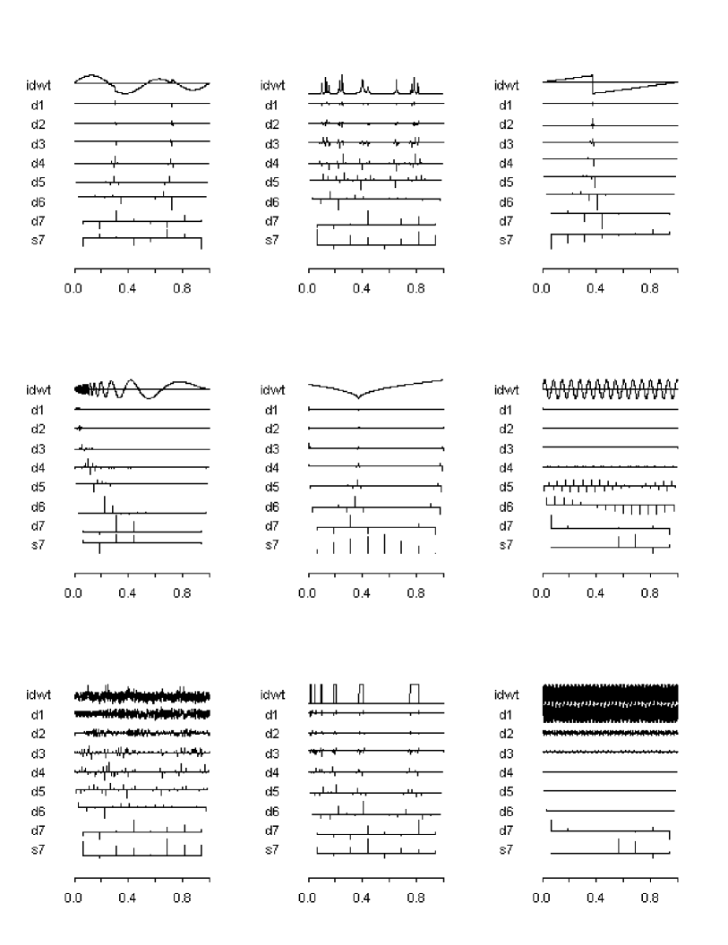
Figure 1: Examples of the discrete wavelet transform of some test functions. There is clear evidence of clustering in most of the graphs. The original functions are shown above their discrete wavelet transform each time.

With this clustering in mind, we model $\xi$ as an area-interaction process on the space $\chi$. The choice of the neighbourhoods $B(x)$ for $x$ in $\chi$ will be discussed below. Given the choice of neighbourhoods, the process will be defined by

$$p(\xi)=\alpha\lambda^{N(\xi)}\gamma^{-m\{U(\xi)\}}$$ (7)

where $p(\xi)$ is the intensity relative to the unit rate independent auto-Poisson process (Cressie,, 1993). If we take $\gamma>1$ this gives a clustered configuration. Thus we would expect to see clusters of large values of $d_{jk}$ if this were a reasonable model — which is exactly what we do see in Figure 1.

A simple application of Bayes theorem tells us that the posterior for our model is

$$p(\xi,\mathbf{d}|\widehat{\mathbf{d}}) = p(\xi)\prod_{j,k}p(d_{jk}|\xi_{jk})\prod_{j,k}p(\widehat{d}_{jk}|d_{jk},\xi_{jk})$$ (8)

$$= \alpha\lambda^{N(\xi)}\gamma^{-m\{U(\xi)\}}\prod_{j,k}\frac{\exp(-d_{jk}^{2}/2\tau^{2}\xi_{jk})}{\sqrt{2\pi\tau^{2}\xi_{jk}}}\prod_{j,k}\frac{\exp\left\{-(\widehat{d}_{jk}-d_{jk})^{2}/2\sigma^{2}\right\}}{\sqrt{2\pi\sigma^{2}}}.$$

Clearly (8) is not a standard density, and in Section 3 we will discuss an extension of coupling from the past which will help us to sample from it.

2.3 Specifying the neighbourhood structure

In order to complete the specification of our area-interaction prior for $\xi$, we need a suitable interpretation of the neighbourhood of a location $x=(j,k)$ on the lattice $\chi$ of indices $(j,k)$ of wavelet coefficients. This lattice is a binary tree, and there are many possibilities. We decided to use the parent, the coefficient on the parent’s level of the transform which is next-nearest to $x$, the two adjacent coefficients on the level of $x$, the two children and the coefficients adjacent to them, making a total of nine coefficients (including $x$ itself). Figure 2 illustrates this scheme, which captures the localisation of both time and frequency effects. Figure 2 also shows how we dealt with boundaries: we assume that the signal we are examining is periodic, making it natural to have periodic boundary conditions in time.

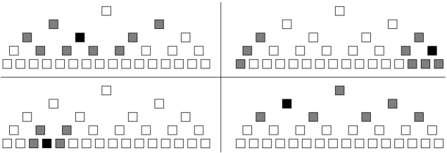
Figure 2: The four plots give examples of what we used as $B(\cdot)$ for four different example locations showing how we dealt with boundaries. Grey boxes are $B(x)\setminus\{x\}$ for each example location $x$, while $x$ itself is shown as black.

If $B(x)$ overlaps with a frequency boundary we simply discard those parts which have no locations associated with them. The simple counting measure used has $m\{B(x)\}=9$ unless $x$ is in the bottom row or one of the top two rows.

Other possible neighbourhood functions include using only the parent, children and immediate sibling and cousin of a coefficient as $B(x)$, or a variation on this taking into account the length of support of the wavelet used. Though we have chosen to use periodic boundary conditions, our method is equally applicable without this assumption.

3 Simulation

In this section, we develop a practical approach to simulation from a close approximation to the posterior density (8). We begin by reviewing the general approach of coupling from the past, and then explore the way in which this concept can be applied to our particular application.

3.1 Coupling from the past

The motivation behind coupling from the past (CFTP) is the following. Suppose that it is desirable to sample from the stationary distribution of an ergodic Markov chain $\{Z_{t}\}$ on some (finite) state space $X$ with states $1,\ldots,n$. It is clear that if it were possible to go back an infinite amount in time, start the chain running (in state $Z_{-\infty}$) and then return to the present, the chain would (with probability 1) be in its stationary distribution when one returned to the present (i.e. $Z_{0}\sim\pi$, where $\pi$ is the stationary distribution of the chain). This is clearly not feasible in practice! Propp and Wilson, (1996) showed that in fact we can achieve the same goal by going back a finite (random) amount of time only.

Consider a finite state space with $n$ states, and that we set not one, but $n$ chains $\{Z^{(1)}_{t}\},\ldots,\{Z^{(n)}_{t}\}$ running at a fixed time $-M$ in the past, where $Z^{(i)}_{-M}=i$ for each chain $\{Z^{(i)}_{t}\}$. Now let all the chains be coupled (see Lindvall,, 1992) so that if $Z^{(i)}_{s}=Z^{(j)}_{s}$ at any time $s$ then $Z^{(i)}_{t}=Z^{(j)}_{t}\hskip 10.00002pt\forall t\geq s$. Then if all the chains ended up in the same state $j$ at time zero (i.e. $Z^{(i)}_{0}=j\hskip 10.00002pt\forall i\in X$), we would know that whichever state a chain passing from time minus infinity to zero was in at time $-M$, the chain would end up in state $j$ at time zero. Thus $j$ must be a sample from the stationary distribution of the Markov chain in question.

Kendall, (1998) extended CFTP to cover simulation of the area-interaction process discussed in Section 2.1, which has an infinite state space. The method makes use of a monotone coupling and stochastic domination. A coupling is monotone if whenever $Z^{(i)}_{t}\geq Z^{(j)}_{t}$ then $Z^{(i)}_{t+k}\geq Z^{(j)}_{t+k}\;\;\forall k>0$. Given a monotone coupling and unique minimum and maximum elements we need only simulate Markov chains starting in the maximum and minimum states and check that these two have coalesced at time $0$, since chains starting in all other states would be sandwiched between these two. As there is no natural maximum element for the area-interaction process, Kendall, used a Poisson process which stochastically dominates the area interaction process of interest to generate a maximum process. More recently, Kendall and Møller, (2000) extended these techniques to more general classes of point processes.

Ambler and Silverman, (2004) explain why the method of Kendall and Møller, (2000) is not practically feasible for some classes of point process models, and provide an alternative method which makes it possible to simulate from densities such as equation (8). We describe their method in the following section.

3.2 Perfect simulation of spatial point processes

We now move to spatial point processes defined on a set like the unit square $[0,1]\times[0,1]\subseteq\mathbb{R}^{2}$. Suppose that we wish to sample from such a spatial point process with density

$$p(X)=\alpha\prod_{i=1}^{m}f_{i}(X),$$

with respect to the unit rate Poisson process, where $\alpha\in(0,\infty)$ and $f_{i}:\mathfrak{R}^{f}\to\mathbb{R}$ are positive valued functions which are (a) monotonic with respect to the partial ordering induced by the subset relation, i.e. for any $X$ and $Y$ related by $X\subseteq Y$, $f_{i}(X)\leq f_{i}(Y)\;\forall i$, and (b) whose conditional intensity

$$\lambda_{f}(u;X)=\frac{f(X\cup\{u\})}{f(X)}$$

is uniformly bounded. Ambler and Silverman, (2004) show that this is possible using the following algorithm.

Let $D$ be a two-dimensional Poisson process with rate equal to

$$\lambda=\prod_{i=1}^{m}\max_{X,\{x\}}\lambda_{f_{i}}(x;X),$$ (9)

evolving over time according to a birth-death process with birth rate equal to (9) and unit death rate. Let $D(T)$ be the configuration of points in process $D$ at time $T$. For simplicity of notation, constrain this function to be right-continuous, so that if there is a birth in $D$ at time $T$ then $D(T)$ is the configuration which existed in $D$ immediately prior to the birth.

Now let $U$ be a birth-death process which is started from an initial configuration equal to that of $D$ at some time in the past, and $L$ be a birth-death process which is started from an initial configuration equal to a thinned version of $D$, where points are accepted with probability

$$\frac{1}{\lambda}\prod_{i=1}^{m}\min_{X,\{x\}}\lambda_{f_{i}}(x;X)$$

The processes $U$ and $L$ evolve through time as follows. If a point $\{u\}$ is born in $D$ at time $T$ then $\{u\}$ is also born in $U$ at time $T$ with probability

$$\frac{1}{\lambda}\prod_{i=1}^{m}\max\left\{\lambda_{f_{i}}[u;U(T)],\lambda_{f_{i}}[u;L(T)]\right\}.$$ (10)

The point $\{u\}$ is born in $L$ at time time $T$ with probability

$$\frac{1}{\lambda}\prod_{i=1}^{m}\min\left\{\lambda_{f_{i}}[u;U(T)],\lambda_{f_{i}}[u;L(T)]\right\}.$$ (11)

If a point dies in $D$ then if it existed in $U$ or $L$ then it dies there also.

Finally, generate $D$ backwards in time from zero to some time $-T$ and start $U$ and $L$ there. Now run them forward to time zero. If $U(0)=L(0)$ then the configuration $U(0)$ (or equivalently $L(0)$) is a sample from the required spatial point process. If not, we must generate $D$ further back in time and try again, keeping the probabilities used for acceptance/rejection in the first round.

In our case, we are simulating from a process on a lattice rather than the unit square, and in the next section, we set out a modified version more appropriate to that context.

3.3 Exact posterior sampling for lattice processes

One of the advantages of the Normal model we propose in Section 2.2 is that it is possible to integrate out $d_{jk}$ and work only with the lattice process $\xi$. Performing this calculation, we see that equation (8) can be rewritten as

$$p(\xi|\widehat{\mathbf{d}}) \!\!\!=\!\!\! p(\xi)\prod_{j,k}\int\frac{\exp(-d_{jk}^{2}/2\tau^{2}\xi_{jk})}{\sqrt{2\pi\tau^{2}\xi_{jk}}}\frac{\exp\left\{-(\widehat{d}_{jk}-d_{jk})^{2}/2\sigma^{2}\right\}}{\sqrt{2\pi\sigma^{2}}}dd_{jk}$$

$$\!\!\!=\!\!\! p(\xi)\prod_{j,k}\int\frac{\exp\left[-\left\{d_{jk}^{2}(\sigma^{2}+\tau^{2}\xi_{jk})-2d_{jk}\widehat{d_{jk}}\tau^{2}\xi_{jk}+\widehat{d_{jk}}\tau^{2}\xi_{jk}\right\}/2\tau^{2}\xi_{jk}\sigma^{2}\right]}{\sqrt{4\pi^{2}\tau^{2}\xi_{jk}\sigma^{2}}}dd_{jk}$$

$$\!\!\!=\!\!\! p(\xi)\prod_{j,k}\frac{\exp\left\{\frac{-\widehat{d_{jk}}^{2}}{2(\sigma^{2}+\tau^{2}\xi_{jk})}\right\}}{\sqrt{4\pi^{2}\tau^{2}\xi_{jk}\sigma^{2}}}\int\exp\left\{-\left(\frac{\sigma^{2}+\tau^{2}\xi_{jk}}{2\tau^{2}\xi_{jk}\sigma^{2}}\right)\left(d_{jk}-\frac{\widehat{d_{jk}}\tau^{2}\xi_{jk}}{\sigma^{2}+\tau^{2}\xi_{jk}}\right)^{2}\right\}dd_{jk}$$

$$\!\!\!=\!\!\! p(\xi)\prod_{j,k}\frac{\exp\left\{\frac{-\widehat{d_{jk}}^{2}}{2(\sigma^{2}+\tau^{2}\xi_{jk})}\right\}}{\sqrt{4\pi^{2}\tau^{2}\xi_{jk}\sigma^{2}}}\left(\frac{2\pi\sigma^{2}\tau^{2}\xi_{jk}}{\sigma^{2}+\tau^{2}\xi_{jk}}\right)^{1/2}$$

$$\!\!\!=\!\!\! p(\xi)\prod_{j,k}\frac{\exp\left\{-\widehat{d_{jk}}^{2}/2(\sigma^{2}+\tau^{2}\xi_{jk})\right\}}{\sqrt{2\pi(\sigma^{2}+\tau^{2}\xi_{jk})}}.$$

We now see that it is possible to sample from the posterior by simulating only the process $\xi$ and ignoring the marks $\mathbf{d}$. This lattice process is amenable to perfect simulation using the method of Ambler and Silverman, (2004). Let

$$f_{1}(\xi)= \;\lambda^{N(\xi)},$$

$$f_{2}(\xi)= \;\gamma^{-m\left\{U(\xi)\right\}},$$

$$f_{3}(\xi)= \;\prod_{j,k}\exp\left\{-\widehat{d_{jk}}^{2}\left/\right.2(\sigma^{2}+\tau^{2}\xi_{jk})\right\}\text{ and}$$

$$f_{4}(\xi)= \;\prod_{j,k}\left\{2\pi(\sigma^{2}+\tau^{2}\xi_{jk})\right\}^{-1/2}.$$

Then

$$\lambda_{f_{1}}(u;\xi)= \;\lambda,$$

$$\lambda_{f_{2}}(u;\xi)= \;\gamma^{-m\left\{B(u)\setminus U(\xi)\right\}}\leq 1,$$

$$\lambda_{f_{3}}(u;\xi)= \;\exp\left[\frac{\widehat{d_{u}}^{2}\tau^{2}}{2(\sigma^{2}+\tau^{2}\xi_{u})\left\{\sigma^{2}+\tau^{2}(\xi_{u}+1)\right\}}\right]\leq\exp\left\{\frac{\widehat{d}_{u}^{2}\tau^{2}}{2\sigma^{2}(\tau^{2}+\sigma^{2})}\right\}\text{ and}$$

$$\lambda_{f_{4}}(u;\xi)= \;\left\{\frac{\tau^{2}\xi_{u}+\sigma^{2}}{\tau^{2}(\xi_{u}+1)+\sigma^{2}}\right\}^{1/2}\leq 1.$$

By a slight abuse of notation, in the second and third equations above we use $u$ to refer both to the point $\{u\}$ and the location $(j,k)$ at which it is found. The functions $f_{1},\ldots,f_{4}$ are also monotone with respect to the subset relation, so all of the conditions for exact simulation using the method of Ambler and Silverman, (2004) are satisfied.

In the spatial processes considered in detail in Ambler and Silverman, (2004), the dominating process had constant intensity across the space $\chi$. In the present context, however, it is necessary in practice to use a dominating process which has a different rate at each lattice location, and then use location-specific maxima and minima rather than global maxima and minima. Because we can now use location-specific, rather than global, maxima and minima, we can initialise upper and lower processes that are much closer together than would have been possible with a constant-rate dominating process, and consequently reducing coalescence times to feasible levels. A constant rate dominating process would not have been feasible due to the size of the global maxima, so this modification to the method of Ambler and Silverman, (2004) is essential; see Section 3.5 for details. Ambler, (2002, Chapter 5) gives some other examples of dominating processes with location-specific intensities.

The location-specific rate of the dominating process $D$ is

$$\lambda_{jk}^{dom}=\lambda e^{\widehat{d}_{jk}^{2}\tau^{2}/2\sigma^{2}(\tau^{2}+\sigma^{2})}$$ (12)

for each location $(j,k)$ on the lattice. The lower process is then started as a thinned version of $D$. Points are accepted with probability

$$P(x)=\gamma^{-M(\chi)}\left(\frac{\sigma^{2}}{\tau^{2}+\sigma^{2}}\right)^{1/2}\times\exp\left\{-\frac{\widehat{d}_{x}^{2}\tau^{2}}{2\sigma^{2}(\tau^{2}+\sigma^{2})}\right\},$$

where $M(\chi)=\max_{\chi}[m\{B(x)\}]$. The upper and lower processes are then evolved through time, accepting points as described in Section 3.2 with probability

$$\frac{1}{\lambda_{jk}^{dom}}\lambda_{f_{1}}(u;\xi^{\text{up}})\lambda_{f_{2}}(u;\xi^{\text{up}})\lambda_{f_{3}}(u;\xi^{\text{low}})\lambda_{f_{4}}(u;\xi^{\text{up}})$$

for the upper process and

$$\frac{1}{\lambda_{jk}^{dom}}\lambda_{f_{1}}(u;\xi^{\text{low}})\lambda_{f_{2}}(u;\xi^{\text{low}})\lambda_{f_{3}}(u;\xi^{\text{up}})\lambda_{f_{4}}(u;\xi^{\text{low}})$$

for the lower process. The remainder of the algorithm carries over in the obvious way. There are still some issues to be addressed due to very high birth rates in the dominating process, and this will be done in Section 3.5.

3.4 Using the generated samples

Although $\mathbf{d}$ was integrated out for simulation reasons in Section 2.2 it is, naturally, the quantity of interest. Having simulated realisations of $\xi|\widehat{\mathbf{d}}$ we then generate $\mathbf{d}|\xi,\widehat{\mathbf{d}}$ for each realisation $\xi$ generated in the first step. The sample median of $\mathbf{d}|\xi,\widehat{\mathbf{d}}$ gives an estimate for $\mathbf{d}$. The median is used instead of the mean as this gives a thresholding rule (defined by Abramovich et al.,, 1998, as a rule giving $p(d_{jk}=0|\widehat{\mathbf{d}})>0$).

We calculate $p(\mathbf{d}|\xi,\widehat{\mathbf{d}})$ using logarithms for ease of notation. Assuming that $\xi_{jk}\neq 0$ we find

$$\log p(d_{jk}|\widehat{d}_{jk},\xi_{jk}\neq 0) = \log{p(d_{jk}|\xi_{jk}\neq 0)}+\log{p(\widehat{d}_{jk}|d_{jk},\xi_{jk}\neq 0)}+C$$

$$= \frac{-d_{jk}^{2}}{2\tau^{2}\xi_{jk}}+\frac{-(\widehat{d}_{jk}-d_{jk})^{2}}{2\sigma^{2}}+C_{1}$$

$$= -\frac{(\sigma^{2}+\tau^{2}\xi_{jk})\left(d_{jk}-\frac{\tau^{2}\xi_{jk}\widehat{d}_{jk}}{\sigma^{2}+\tau^{2}\xi_{jk}}\right)^{2}}{2\sigma^{2}\tau^{2}\xi_{jk}}+C_{2}$$

where $C$, $C_{1}$ and $C_{2}$ are constants. Thus

$$d_{jk}|\widehat{d}_{jk},\xi_{jk}\neq 0\sim N\left(\frac{\tau^{2}\xi_{jk}\widehat{d}_{jk}}{\sigma^{2}+\tau^{2}\xi_{jk}},\frac{\sigma^{2}\tau^{2}\xi_{jk}}{\sigma^{2}+\tau^{2}\xi_{jk}}\right).$$

When $\xi_{jk}=0$ we clearly have $p(d_{jk}|\xi_{jk},\widehat{d}_{jk})=0$.

3.5 Dealing with large and small rates

We now deal with some approximations which are necessary to allow our algorithm to be feasible computationally. Recall from equation (12) that if the maximum data value $d_{jk}$ is twenty times larger in magnitude than the standard deviation of the noise (a not uncommon event for reasonable noise levels) then we have

$$\lambda_{dom} = \lambda e^{400\sigma^{2}\tau^{2}/2\sigma^{2}(\tau^{2}+\sigma^{2})}$$

$$= \lambda e^{200\tau^{2}/(\tau^{2}+\sigma^{2})}.$$

Now unless $\tau$ is significantly smaller than $\sigma$, this will result in enormous birth rates, which make it necessary to modify the algorithm appropriately. To address this issue, we noted that the chances of there being no live points at a location whose data value is large (resulting in a value of $\lambda_{dom}$ larger than $e^{4}$) is sufficiently small that for the purposes of calculating $\lambda_{f_{2}}(u;\xi)$ for nearby locations it can be assumed that the number of points alive was strictly positive.

This means that we do not know the true value of $\xi_{jk}$ for the locations with the largest values of $d_{jk}$. This leads to problems since we need to generate $d_{jk}$ from the distribution

$$d_{jk}|\xi_{jk},\widehat{d}_{jk}\sim N\left(\frac{\tau^{2}\xi_{jk}\widehat{d}_{jk}}{\sigma^{2}+\tau^{2}\xi_{jk}},\frac{\sigma^{2}\tau^{2}\xi_{jk}}{\sigma^{2}+\tau^{2}\xi_{jk}}\right),$$

which requires values of $\xi_{jk}$ for each location $(j,k)$ in the configuration. To deal with this issue, we first note that

$$\frac{\tau^{2}\xi_{jk}\widehat{d}_{jk}}{\sigma^{2}+\tau^{2}\xi_{jk}}\hskip 5.0pt\mathop{-\!\!\!\longrightarrow}_{\xi_{jk}\to\infty}\hskip 5.0pt\widehat{d}_{jk}$$

monotonically from below, and that

$$\frac{\tau^{2}\xi_{jk}\sigma^{2}}{\sigma^{2}+\tau^{2}\xi_{jk}}\hskip 5.0pt\mathop{-\!\!\!\longrightarrow}_{\xi_{jk}\to\infty}\hskip 5.0pt\sigma^{2},$$

also monotonically from below. Since $\sigma$ is typically small, convergence is very fast indeed. Taking $\tau=\sigma$ as an example we see that even when $\xi_{jk}=5$ we have

$$\frac{\tau^{2}\xi_{jk}\widehat{d}_{jk}}{\sigma^{2}+\tau^{2}\xi_{jk}}=\frac{5}{6}\widehat{d}_{jk}$$

and

$$\frac{\tau^{2}\xi_{jk}\sigma^{2}}{\sigma^{2}+\tau^{2}\xi_{jk}}=\frac{5}{6}\sigma^{2}.$$

We see that we are already within $\frac{1}{6}$ of the limit. Convergence is even faster for larger values of $\tau$.

We also recall that the dominating process gives an upper bound for the value of $\xi_{jk}$ at every location. Thus a good estimate for $d_{jk}$ would be gained by taking the value of $\xi_{jk}$ in the dominating process for those points where we do not know the exact value. This is a good solution but is unnecessary in some cases, as sometimes the value of $\lambda_{dom}$ is so large that there is little advantage in using this value. Thus for exceptionally large values of $\lambda_{dom}$ we simply use $N(\widehat{d}_{jk},\sigma^{2})$ numbers as our estimate of $d_{jk}$.

4 Simulation Study

We now present a simulation study of the performance of our estimator relative to several established Wavelet-based estimators. Similar to the study of Abramovich et al., (1998), we investigate the performance of our method on the four standard test functions of Donoho and Johnstone, (1994, 1995), namely “Blocks”, “Bumps”, “Doppler” and “Heavisine”. These test functions are used because they exhibit different kinds behaviour typical of signals arising in a variety of applications.

The test functions were simulated at 256 points equally spaced on the unit interval. The test signals were centred and scaled so as to have mean value $0$ and standard deviation $1$. We then added independent $N(0,\sigma^{2})$ noise to each of the functions, where $\sigma$ was taken as $1/10$, $1/7$ and $1/3$. The noise levels then correspond to root signal-to-noise ratios (RSNR) of $10$, $7$ and $3$ respectively. We performed 25 replications. For our method, we simulated 25 independent draws from the posterior distribution of the $d_{jk}$’s and used the sample median as our estimate, as this gives a thresholding rule. For each of the runs, $\sigma$ was set to the standard deviation of the noise we added, $\tau$ was set to $1.0$, $\lambda$ was set to $0.05$ and $\gamma$ was set to $3.0$.

The values of parameters $\sigma$ and $\tau$ were set to the true values of the standard deviation of the noise and the signal, respectively. In practice it will be necessary to develop some method for estimating these values. The value of $\lambda$ was chosen to be $0.05$ because it was felt that not many of the coefficients would be significant. The value of $\gamma$ was chosen based on small trials for the heavisine and jumpsine datasets.

We compare our method with several established wavelet-based estimators for reconstructing noisy signals: SureShrink (Donoho and Johnstone,, 1994), two-fold cross-validation as applied by Nason, (1996), ordinary BayesThresh (Abramovich et al.,, 1998), and the false discovery rate as applied by Abramovich and Benjamini, (1996).

For test signals “Bumps”, “Doppler” and “Heavisine” we used Daubechies least asymmetric wavelet of order 10 (Daubechies,, 1992). For “Blocks” we used the Haar wavelet, as the original signal was piecewise constant. The analysis was carried out using the freely available $R$ statistical package. The WaveThresh package (Nason,, 1993) was used to perform the discrete wavelet transform and also to compute the SureShrink, cross-validation, BayesThresh and false discovery rate estimators.

Table 1: Average mean-square errors ($\times 10^{4}$) for the area-interaction BayesThresh (AIBT), SureShrink (SS), cross-validation (CV), ordinary BayesThresh (BT) and false discovery rate (FDR) estimators for four test functions for three values of the root signal-to-noise ratio. Averages are based on 25 replicates. Standard errors are given in parentheses.

RSNR	Method	Test functions
		Blocks		Bumps		Doppler		Heavisine
	AIBT	25	(1)	84	(2)	49	(1)	32	(1)
	SS	49	(2)	131	(6)	54	(2)	66	(2)
10	CV	55	(2)	392	(21)	112	(5)	31	(1)
	BT	344	(10)	1651	(17)	167	(5)	35	(2)
	FDR	159	(14)	449	(17)	145	(5)	64	(3)
	AIBT	56	(3)	185	(5)	87	(3)	52	(2)
	SS	98	(3)	253	(10)	99	(4)	94	(4)
7	CV	96	(3)	441	(25)	135	(6)	54	(3)
	BT	414	(11)	1716	(21)	225	(6)	57	(2)
	FDR	294	(18)	758	(27)	253	(9)	93	(4)
	AIBT	535	(21)	1023	(15)	448	(18)	153	(6)
	SS	482	(13)	973	(45)	399	(14)	147	(3)
3	CV	452	(11)	914	(34)	375	(13)	148	(6)
	BT	860	(24)	2015	(37)	448	(12)	140	(4)
	FDR	1230	(52)	2324	(88)	862	(31)	148	(3)

The goodness of fit of each estimator was measured by its average mean-square error (AMSE) over the 25 replications. Table 1 presents the results. It is clear that our estimator performs extremely well with respect to the other estimators when the signal-to-noise ratio is moderate or large, but less well, though still competitively, when there is a small signal-to-noise ratio.

5 Conclusions and future work

We have introduced a procedure for Bayesian wavelet thresholding which uses the naturally clustered nature of the wavelet transform when deciding how much weight to give coefficient values. In comparisons with other methods, our approach performed very well for moderate and low noise levels, and reasonably competitively for higher noise levels.

One possible area for future work would be to replace equation (6) with

$$d_{jk}|\xi\sim N(0,\tau^{2}(\xi_{jk})^{z}),$$

where $z$ would be a further parameter. This would modify the number of points which are likely to be alive at any given location and thus also modify the tail behaviour of the prior. The idea behind this suggestion is that when we know that the behaviour of the data is either heavy or light tailed, we could adjust $z$ to compensate. This could possibly also help speed up convergence by reducing the number of points at locations with large values of $d_{jk}$. As inclusion of this extra parameter requires only minor modifications, the software discussed actually includes this option. The results presented in Section 4 were generated by simply setting $z=1$.

A second possible area for future work would be to develop some automatic methods for choosing the parameter values, perhaps using the method of maximum pseudo-likelihood (Besag,, 1974, 1975, 1977).

Software implementing the work described in this paper is available on request from the first author.

6 Acknowledgements

The first author would like to thank Guy Nason and Paul Northrop for helpful discussions.

References

- Abramovich and Benjamini, (1996) Abramovich, F. and Benjamini, Y. (1996). Adaptive thresholding of wavelet coefficients. Computational Statistics and Data Analysis, 22:351–361.
- Abramovich et al., (1998) Abramovich, F., Sapatinas, T., and Silverman, B. W. (1998). Wavelet thresholding via a Bayesian approach. Journal of the Royal Statistical Society, Series B, 60:725–749.
- Ambler, (2002) Ambler, G. K. (2002). Dominated Coupling from the Past and Some Extensions of the Area-Interaction Process. PhD thesis, Department of Mathematics, University of Bristol.