Abstract

In this paper we extend a recent result of Collin-Rosenberg (a solution for the minimal surface equation in the Euclidean disc has radial limits almost everywhere) for a large class of differential operators in Divergence form. Also, we give an alternative proof of Fatou’s Theorem (a harmonic function defined in the Euclidean disc has radial limits almost everywhere) even for harmonic functions that are not bounded. Moreover, we construct an example (in the spirit of [3]) of a minimal graph in $\mathbb{M}^{2}\times\mathbb{R}$, where $\mathbb{M}^{2}$ is a Hadamard surface, over a geodesic disc which has finite radial limits in a mesure zero set.

1 Introduction

It is well known that a bounded harmonic function $u$ defined on the Euclidean disc $D$ has radial limits almost everywhere (Fatou’s Theorem [4]). Moreover, the radial limits can not be plus infinity for a positive measure set. For fixed $\theta\in\hbox{\bb S}^{n-1}$, the radial limit $u(\theta)$ (if it exists) is defined as

$$u(\theta)=\lim_{r\to 1}u(r,\theta),$$

where we paramatrize the Euclidean disc in polar coordinates $(r,\theta)\in[0,1)\times\hbox{\bb S}^{1}$.

In 1965, J. Nitsche [8] asked if a Fatou Theorem is valid for the minimal surface equation, i.e., does a solution for the minimal surface equation in the Euclidean disc have radial limits almost everywhere? This question has been solved recently by P. Collin and H. Rosenberg [3]. Moreover, in the same paper [8], J. Nitsche asked: what is the largest set of $\theta$ for which a minimal graph on $D$ may not have radial limits? Again, this question was solved in [3] if one allows infinite radial limits. That is, they construct an example of a minimal graph in the Euclidean disc with finite radial limits only on a set of measure zero. In this example, the $+\infty$ radial limits (resp. $-\infty$) are taken on a set of measure $\pi$ (resp. $\pi$).

The aim of this paper is to extend both results and give an alternative proof of Fatou’s Theorem for a more general situation. In Section 2, we extend Collin-Rosenberg’s Theorem for a large class of differential operators in divergence form (see Theorem 2.1). Also, we extend Fatou’s Theorem even for harmonic functions that are not bounded (see Theorem 2.2). In particular, as a consequence of this result, we obtain the classical Fatou Theorem (see Corollary 2.1). In Section 3, we construct an example of a minimal graph in $\mathbb{M}^{2}\times\mathbb{R}$ over a geodesic disk $\mathcal{D}\subset\mathbb{M}^{2}$ ($\mathbb{M}^{2}$ is a Hadamard surface) for which the finite radial limits are of measure zero. Also, the $+\infty$ radial limits (resp. $-\infty$) are taken on a set of measure $\pi$ (resp. $\pi$).

2 Fatou’s Theorem

Henceforth $(\hbox{\bb B},g)$ denotes the $n-$dimensional unit open ball, i.e,

$$\hbox{\bb B}=\left\{(r,\theta)\,;\,0\leq r<1,\,\theta\in\hbox{\bb S}^{n-1}\right\},$$

in polar coordinates with respect to $g$, $g$ a $C^{2}-$Riemannian metric on 𝔹. Define $G:=G(r,\theta)=\sqrt{{\rm det}(g)}$. Moreover, we denote by $\nabla$ the Levi-Civita connection associated to $g$ and by ${\rm div}_{g}$ its associated divergence operator. Also, $L^{1}(\hbox{\bb B})$ denotes the set of integrable functions on $(\hbox{\bb B},g)$.

Set $u\in C^{2}(\hbox{\bb B})-$function and $X_{u}$ be a $C^{1}(\hbox{\bb B})-$vector field so that its coordinates depend on $u$, its first derivatives and $C^{1}(\hbox{\bb B})-$functions.

For fixed $\theta\in\hbox{\bb S}^{n-1}$, the radial limit ( if it exists) $u(\theta)$ is defined as

$$u(\theta)=\lim_{r\to 1}u(r,\theta).$$

Theorem 2.1.

Let $(\hbox{\bb B},g,G,u,X_{u})$ be as above. Assume that

• $\alpha\leq G(r,\theta)\leq\beta$ for all $(r,\theta)\in[0,1)\times\hbox{\bb S}^{n-1}$, $\alpha$ and $\beta$ positive constants.

• $|X_{u}|\leq M$ on 𝔹, i.e., $X_{u}$ is bounded on 𝔹.

• $g(\nabla u,X_{u})\geq\delta\,|\nabla u|+h$, where $\delta$ is a positive constant and $h\in L^{1}(\hbox{\bb B})$.

Let $f\in L^{1}(\hbox{\bb B})$. If $u$ is a solution of

$${\rm div}_{g}(X_{u})\geq\,(\,\text{ or }\,\leq\,)\,f\,\text{ on }\,\hbox{\bb B},$$

then $u$ has radial limits almost everywhere.

Proof.

First, let us prove the case

$${\rm div}_{g}(X_{u})\geq\,\,f.$$

For $r<1$ fixed, set $\hbox{\bb B}(r)$ the $n-$dimensional open ball of radius $r$. Let $\eta:\hbox{\bb R}\longrightarrow(0,+1)$ be a smooth function so that $0<\eta^{\prime}(x)<1$ for all $x\in\hbox{\bb R}$. Define $\psi:=\eta\circ u$.

On the one hand, by direct computations and item c), we have

$$\begin{split}{\rm div}_{g}(\psi\,X_{u})&=\psi\,{\rm div}_{g}(X_{u})+g(\nabla\psi,X_{u})\geq\psi\,f+\eta^{\prime}\,g(\nabla u,X_{u})\\[8.53581pt] &\geq\psi\,f+\eta^{\prime}\,\left(\delta\,|\nabla u|+h\right)=\delta\,\eta^{\prime}\,|\nabla u|+\left(\psi\,f+\eta^{\prime}\,h\right)\\ &=\delta\,|\nabla\psi|+\left(\psi\,f+\eta^{\prime}\,h\right),\end{split}$$

thus

$$\int_{\hbox{\bbt B}(r)}{\rm div}_{g}(\psi\,X_{u})\geq\delta\int_{\hbox{\bbt B}(r)}|\nabla\psi|+C$$ (2.1)

where $C$ is some constant. This follows since $f$ and $h$ are $L^{1}-$functions on 𝔹.

On the other hand, by Stokes’ Theorem and items a) and ${\it b)}$, we obtain for $r<1$ fixed

$$\begin{split}\int_{\hbox{\bbt B}(r)}{\rm div}_{g}(\psi\,X_{u})&=\int_{\partial\hbox{\bbt B}(r)}\psi\,g(X_{u},\upsilon)\leq\int_{\partial\hbox{\bbt B}(r)}M\\ &=M\int_{\theta\in\hbox{\bbt S}^{n-1}}G(r,\theta)d\theta\leq M\,\beta\int_{\theta\in\hbox{\bbt S}^{n-1}}\\ &=M\,\beta\,\omega_{n-1},\end{split}$$ (2.2)

where $\upsilon$ is the outer conormal to $\partial\hbox{\bb B}(r)$ and $\omega_{n-1}$ is the volume of $\hbox{\bb S}^{n-1}$.

So, from (2.1), (2.2) and letting $r$ go to one, we conclude that $|\nabla\psi|$ is integrable in 𝔹, i.e.,

$$\int_{\hbox{\bbt B}}|\nabla\psi|<+\infty$$ (2.3)

Since $\dfrac{\partial\psi}{\partial r}\leq|\nabla\psi|$, we have from Fubini’s Theorem and (2.3)

$$\int_{\hbox{\bbt B}}\dfrac{\partial\psi}{\partial r}=\int_{\theta\in\hbox{\bbt S}^{n-1}}\left(\int_{0}^{1}\dfrac{\partial\psi}{\partial r}G(r,\theta)\,dr\right)d\theta<\infty.$$

Thus, as $G(r,\theta)$ is bounded below by a positive constant, for almost all $\theta\in\hbox{\bb S}^{n-1}$,

$$\lim_{r\to 1}\psi(r,\theta)-\psi(0,0)=\int_{0}^{1}\dfrac{\partial\psi}{\partial r}(r,\theta)dr<\infty,$$

that is, $\psi$ has radial limits almost everywhere. Since $\psi=\eta\circ u$, we conclude $u$ has radial limits almost everywhere (which may be $\pm\infty$).

For

$${\rm div}_{g}(X_{u})\leq f,$$

we just have to follow the above proof by changing $\eta:\hbox{\bb R}\longrightarrow(-1,0)$ so that $0<\eta^{\prime}(x)<1$ for all $x\in\hbox{\bb R}$. ∎

As we pointed out in the Introduction, in the spirit of Theorem 2.1, we can give an alternative proof of Fatou’s Theorem even for harmonic function that are not bounded, i.e.,

Theorem 2.2.

Let $(\hbox{\bb B},g,G,u)$ be as above. Assume that $\alpha\leq G(r,\theta)\leq\beta$ for all $(r,\theta)\in[0,1)\times\hbox{\bb S}^{n-1}$, $\alpha$ and $\beta$ positive constants. If $u$ is a solution of

$${\rm div}_{g}(\nabla u)=\,0\,\text{ on }\,\hbox{\bb B},$$

then $u$ has radial limits almost everywhere.

Proof.

For $r<1$ fixed, set $\hbox{\bb B}(r)$ the $n-$dimensional open ball of radius $r$. Let $\eta:\hbox{\bb R}\longrightarrow(0,1)$ be a smooth function so that $0<\eta^{\prime}(x)<1$ for all $x\in\hbox{\bb R}$. Define

$$\phi:=\eta\circ u,\mbox{ and }\psi:=\dfrac{\phi}{\sqrt{1+\left|\nabla u\right|^{2}}}.$$

On the one hand, by direct computations, we have

$$\begin{split}{\rm div}_{g}(\psi\,\nabla u)&=\psi\,{\rm div}_{g}(\nabla u)+\langle\nabla\psi,\nabla u\rangle=\langle\nabla\psi,\nabla u\rangle\\[8.53581pt] &=\eta^{\prime}\dfrac{\left|\nabla u\right|^{2}}{\sqrt{1+\left|\nabla u\right|^{2}}}-\phi\dfrac{\langle\nabla\left|\nabla u\right|^{2},\nabla u\rangle}{2(1+\left|\nabla u\right|^{2})^{3/2}}\\[8.53581pt] &\geq\eta^{\prime}\left|\nabla u\right|-\dfrac{\eta^{\prime}}{\sqrt{1+\left|\nabla u\right|^{2}}}-\phi\dfrac{\langle\nabla\left|\nabla u\right|^{2},\nabla u\rangle}{2(1+\left|\nabla u\right|^{2})^{3/2}}\\[8.53581pt] &\geq\left|\nabla\phi\right|-1-\dfrac{\langle\nabla\left|\nabla u\right|^{2},\nabla u\rangle}{2(1+\left|\nabla u\right|^{2})^{3/2}},\end{split}$$

since

$$\nabla\psi=\eta^{\prime}\dfrac{\nabla u}{\sqrt{1+\left|\nabla u\right|^{2}}}-\phi\dfrac{\nabla\left|\nabla u\right|^{2}}{2(1+\left|\nabla u\right|^{2})^{3/2}}.$$

Let us first bound the term

$$\left|\int_{\hbox{\bbt B}(r)}\dfrac{\langle\nabla\left|\nabla u\right|^{2},\nabla u\rangle}{2(1+\left|\nabla u\right|^{2})^{3/2}}\right|.$$

Set $Y_{u}:=\dfrac{\nabla u}{\sqrt{1+\left|\nabla u\right|^{2}}}$, then

$$\begin{split}{\rm div}_{g}(Y_{u})&=\dfrac{1}{\sqrt{1+\left|\nabla u\right|^{2}}}{\rm div}_{g}(\nabla u)-\dfrac{\langle\nabla\left|\nabla u\right|^{2},\nabla u\rangle}{2(1+\left|\nabla u\right|^{2})^{3/2}}\\ &=-\dfrac{\langle\nabla\left|\nabla u\right|^{2},\nabla u\rangle}{2(1+\left|\nabla u\right|^{2})^{3/2}}\end{split}$$

since ${\rm div}_{g}(\nabla u)=0$. Applying Stoke’s Theorem we obtain

$$\int_{\hbox{\bbt B}(r)}{\rm div}_{g}(Y_{u})=\int_{\partial\hbox{\bbt B}(r)}\langle Y_{u},\upsilon\rangle,$$

that is

$$\begin{split}\left|\int_{\hbox{\bbt B}(r)}\dfrac{\langle\nabla\left|\nabla u\right|^{2},\nabla u\rangle}{2(1+\left|\nabla u\right|^{2})^{3/2}}\right|&=\left|\int_{\partial\hbox{\bbt B}(r)}\langle Y_{u},\upsilon\rangle\right|\leq\int_{\partial\hbox{\bbt B}(r)}\left|Y_{u}\right|\\[8.53581pt] &=\int_{\partial\hbox{\bbt B}(r)}\dfrac{\left|\nabla u\right|}{\sqrt{1+\left|\nabla u\right|^{2}}}\leq\int_{\partial\hbox{\bbt B}(r)}\leq C,\end{split}$$

for some positive constant $C$.

Thus

$$\int_{\hbox{\bbt B}(r)}{\rm div}(\psi\,X_{u})\geq\int_{\hbox{\bbt B}(r)}|\nabla\phi|-\tilde{C},$$ (2.4)

for some positive constant $\tilde{C}$.

On the other hand, by Stokes’ Theorem we obtain for $r<1$ fixed

$$\begin{split}\int_{\hbox{\bbt B}(r)}{\rm div}(\psi\,X_{u})&=\int_{\partial\hbox{\bbt B}(r)}\psi\,\langle X_{u},\upsilon\rangle\leq\int_{\partial\hbox{\bbt B}(r)}\frac{\left|\nabla u\right|}{\sqrt{1+\left|\nabla u\right|^{2}}}\\ &\leq\int_{\partial\hbox{\bbt B}(r)}\leq C^{\prime},\end{split}$$ (2.5)

where $\upsilon$ is the outer conormal to $\partial\hbox{\bb B}(r)$ and $C^{\prime}$ is some positive constant.

So, from (2.4), (2.5) and letting $r$ go to one, we conclude that $|\nabla\phi|$ is integrable in 𝔹, i.e.,

$$\int_{\hbox{\bbt B}}|\nabla\phi|<\infty$$ (2.6)

Since $\dfrac{\partial\phi}{\partial r}\leq|\nabla\phi|$, we have from Fubini’s Theorem and (2.6)

$$\int_{\hbox{\bbt B}}\dfrac{\partial\phi}{\partial r}=\int_{\theta\in\hbox{\bbt S}^{1}}\left(\int_{0}^{1}\dfrac{\partial\phi}{\partial r}G(r,\theta)\,dr\right)d\theta<\infty.$$

Thus, as $G(r,\theta)$ is bounded below by a positive constant, for almost all $\theta\in\hbox{\bb S}^{n-1}$,

$$\lim_{r\to 1}\phi(r,\theta)-\phi(0,0)=\int_{0}^{1}\dfrac{\partial\phi}{\partial r}(r,\theta)dr<\infty,$$

that is, $\phi$ has radial limits almost everywhere. Since $\phi=\eta\circ u$, we conclude $u$ has radial limits almost everywhere (which may be $\pm\infty$). ∎

Then, as a consequence

Corollary 2.1.

Let $u$ be a harmonic function defined over the Euclidean disc. Then $u$ has radial limits almost everywhere.

2.1 Applications

Moreover, we will see now how Theorem 2.1 applies to get radial limits almost everywhere for minimal graphs in ambient spaces besides $\hbox{\bb R}^{3}$. We work here in Heisenberg space, but it is not hard to check that we could work with minimal graphs in a more general submersion (see [7]).

First, we need to recall some definitions in Heisenberg space (see [1]). The Heisenberg spaces are $\hbox{\bb R}^{3}$ endowed with a one parameter family of metrics indexed by bundle curvature by a real parameter $\tau\neq 0$. When we say the Heisenberg space, we mean $\tau=1/2$, and we denote it by $\mathcal{H}$.

In global exponential coordinates, $\mathcal{H}$ is $\hbox{\bb R}^{3}$ endowed with the metric

$$g=(dx^{2}+dy^{2})+(\frac{1}{2}(ydx-xdy)+dz)^{2}.$$

The Heisenberg space is a Riemannian submersion $\pi:\mathcal{H}\longrightarrow\hbox{\bb R}$ over the standard flat Euclidean plane $\hbox{\bb R}^{2}$ whose fibers are the vertical lines, i.e., they are the trajectories of a unit Killing vector field and hence geodesics.

Let $S_{0}\subset\mathcal{H}$ be the surface whose points satisfy $z=0$. Let $D\subset\hbox{\bb R}^{2}$ be the unit disc. Henceforth, we identify domains in $\hbox{\bb R}^{2}$ with its lift to $S_{0}$. The Killing graph of a function $u\in C^{2}(D)$ is the surface

$$\Sigma=\left\{(x,y,u(x,y))\,;\,(x,y)\in D\right\}.$$

Moreover, the minimal graph equation is

$${\rm div}_{\hbox{\bbt R}^{2}}(X_{u})=0,$$

here ${\rm div}_{\hbox{\bbt R}^{2}}$ stands for the divergence operator in $\hbox{\bb R}^{2}$ with the Euclidean metric $\langle,\rangle$, and

$$X_{u}:=\frac{\alpha}{W}\partial_{x}+\frac{\beta}{W}\partial_{y},$$

where

$$\alpha:=\frac{y}{2}+u_{x},\quad\beta:=-\frac{x}{2}+u_{y},$$

and

$$W^{2}=1+\alpha^{2}+\beta^{2}.$$

Thus, for verifying $u$ has radial limits almost everywhere (which may be $\pm\infty$), we have to check conditions $a)$, $b)$ and $c)$. Item $a)$ is immediate since we are working with the Euclidean metric.

Item $b)$ follows from

$$\left|X_{u}\right|^{2}=\frac{\alpha^{2}+\beta^{2}}{1+\alpha^{2}+\beta^{2}}\leq 1.$$

Now, we need to check Item $c)$. On one hand, using polar coordinates $x=r\cos\theta$ and $y=r\sin\theta$, we have

$$\begin{split}W^{2}&=1+\alpha^{2}+\beta^{2}=1+u_{x}^{2}+u_{y}^{2}+(yu_{x}-xu_{y})+\frac{x^{2}+y^{2}}{4}\\ &=1+|\nabla u|^{2}+\langle\nabla u,(-y,x)\rangle+\frac{x^{2}+y^{2}}{4}\\ &\geq 1+|\nabla u|^{2}-|\nabla u||(-y,x)|+\frac{x^{2}+y^{2}}{4}\\ &=1+|\nabla u|^{2}-r|\nabla u|+\frac{r^{2}}{4}\end{split}$$

thus,

$$W\geq\sqrt{1+\left(|\nabla u|-\frac{r}{2}\right)^{2}}\geq\left||\nabla u|-\frac{r}{2}\right|.$$

We need a lower bound for $W$ in terms of $|\nabla u|$. To do so, we distinguish two cases:

Case $|\nabla u|\leq 5/4$: Since

$$1-r\left|\nabla u\right|+\frac{r^{2}}{4}\geq 1-\frac{5r}{4}+\frac{r^{2}}{4}\geq 0\mbox{ for all }r\leq 1,$$

we obtain

$$W\geq\sqrt{\left|\nabla u\right|^{2}+1-r\left|\nabla u\right|+\frac{r^{2}}{4}}\geq\left|\nabla u\right|.$$

Case $\left|\nabla u\right|>5/4$: We already know that

$$W\geq\left||\nabla u|-\frac{r}{2}\right|,$$

thus, for $\left|\nabla u\right|>5/4$, it is easy to see that

$$\left||\nabla u|-\frac{r}{2}\right|\geq\frac{3}{10}\left|\nabla u\right|\mbox{ for all }r\leq 1.$$

So, in any case, for $\delta=3/10>0$

$$W\geq\delta\left|\nabla u\right|.$$ (2.7)

On the other hand,

$$\begin{split}\langle\nabla u,X_{u}\rangle&=\frac{u_{x}^{2}+u_{y}^{2}+\frac{1}{2}(yu_{x}-xu_{y})}{W}\\[11.38109pt] &=\frac{1+u_{x}^{2}+u_{y}^{2}+(yu_{x}-xu_{y})+\frac{x^{2}+y^{2}}{4}}{W}-\frac{1+\frac{1}{2}(yu_{x}-xu_{y})+\frac{x^{2}+y^{2}}{4}}{W}\\[11.38109pt] &=\frac{W^{2}}{W}+h=W+h\geq\delta\left|\nabla u\right|+h,\end{split}$$

where we have used (2.7) and $h$ denotes the $L^{1}(D)-$function

$$h=-\frac{1+\frac{1}{2}(yu_{x}-xu_{y})+\frac{x^{2}+y^{2}}{4}}{\sqrt{1+u_{x}^{2}+u_{y}^{2}+(yu_{x}-xu_{y})+\frac{x^{2}+y^{2}}{4}}},$$

that is, Item $c)$ is satisfied. So,

Corollary 2.2.

A solution for the minimal surface equation in the Heisenberg space defined over a disc has radial limits almost everywhere (which may be $\pm\infty$).

3 An example in a Hadamard surface

The aim of this Section is to construct an example of a minimal graph in $\mathbb{M}^{2}\times\mathbb{R}$ over a geodesic disk $\mathcal{D}\subset\mathbb{M}^{2}$ ($\mathbb{M}^{2}$ is a Hadamard surface) for which the finite radial limits are of measure zero.

We need to recall preliminary facts about graphs over a Hadamard surface (see [5] for details). Henceforth, $\mathbb{M}^{2}$ denotes a simply connected with Gauss curvature bounded above by a negative constant, i.e., $K_{\hbox{\bbt M}^{2}}\leq c<0$.

Let $p_{0}\in\mathbb{M}^{2}$ and $\mathcal{D}$ be the the geodesic disk in $\mathbb{M}^{2}$ centered at $p_{0}$ of radius one. Re-scaling in the metric, we can assume that

$${\rm max}\left\{K_{\hbox{\bbt M}^{2}}(p)\,;\,\,p\in\overline{\mathcal{D}}\right\}=-1.$$

From the Hessian Comparison Theorem (see e.g. [6]), $\partial\mathcal{D}$ bounds a strictly convex domain. We assume that $\partial\mathcal{D}$ is smooth, otherwise we can work in a smaller disc. We identify $\partial\mathcal{D}=\hbox{\bb S}^{1}$ and orient it counter-clockwise.

We say that $\Gamma$ is an admissible polygon in $\mathcal{D}$ if $\Gamma$ is a Jordan curve in $\overline{\mathcal{D}}$ which is a geodesic polygon with an even number of sides and all the vertices in $\partial\mathcal{D}$. We denote by $A_{1},B_{1},\ldots,A_{k},B_{k}$ the sides of $\Gamma$ which are oriented counter-clockwise. Recall that any two sides can not intersect in $\mathcal{D}$. Set $D$ the domain in $\mathcal{D}$ bounded by $\Gamma$. By $|A_{i}|$ (resp. $|B_{j}|$), we denote the length of such a geodesic arc.

Theorem 3.1 ([9]).

Let $\Gamma\subset\mathbb{M}^{2}$ be a compact polygon with an even number of geodesic sides $A_{1},B_{1},A_{2},B_{2},\ldots,A_{n},B_{n}$, in that order, and denote by $D$ the domain with $\partial D=\Gamma$. The necessary and sufficient conditions for the existence of a minimal graph $u$ on $D$, taking values $+\infty$ on each $A_{i}$, and $-\infty$ on each $B_{j}$, are the two following conditions:

1. $\sum_{i=1}^{n}|A_{i}|=\sum_{i=1}^{n}|B_{i}|$,

2. for each inscribed polygon $P$ in $D$ (the vertices of $P$ are among the vertices of $\Gamma$) $P\neq D$, one has the two inequalities:

   $$2a(P)<|P|\mbox{ and }2b(P)<|P|.$$

Here $a(P)=\sum_{A_{j}\in P}|A_{j}|$, $b(P)=\sum_{B_{j}\in P}|B_{j}|$ and $|P|$ is the perimeter of $P$.

The construction of this example follows the steps in [3, Section III], but here we have to be more careful in the choice of the first inscribed square and the trapezoids. We need to choose them as symmetric as possible.

Let us first explain how we take the inscribed square: Let $L={\rm length}(\partial\mathcal{D})$ and $\gamma(x_{0},x_{1})$ be the geodesic arc in $\mathcal{D}$ joining $x_{0},x_{1}\in\partial\mathcal{D}$. Fix $x_{0}\in\partial\mathcal{D}$ and let $\alpha:\hbox{\bb R}/[0,L)\longrightarrow\partial\mathcal{D}$ an arc-length parametrization of $\partial\mathcal{D}$ (oriented count-clockwise). Set $x_{1}=\alpha(L/2)$. Consider $x_{0}^{\pm}(s)=\alpha(\pm s)$ and $x_{1}^{\pm}(s)=\alpha(L/2\pm s)$ for $0\leq s\leq L/2$ (c.f. Figure 1), and denote

$$B_{1}(s) = \gamma(x_{0}^{+}(s),x_{1}^{-}(s))$$

$$A_{1}(s) = \gamma(x_{1}^{-}(s),x_{1}^{+}(s))$$

$$B_{2}(s) = \gamma(x_{1}^{+}(s),x_{0}^{-}(s))$$

$$A_{2}(s) = \gamma(x_{0}^{-}(s),x_{1}^{+}(s)).$$

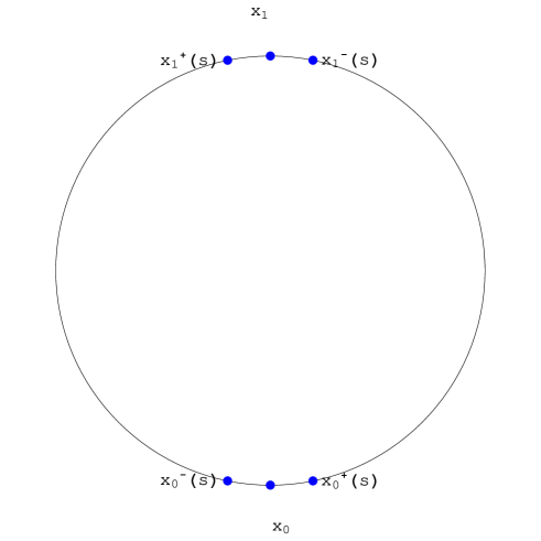
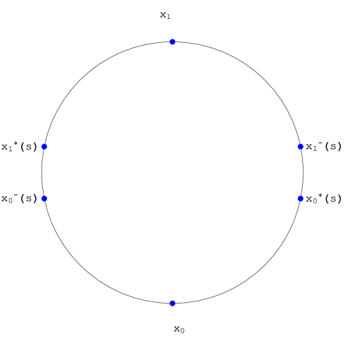
Figure 1: We move the points along $\partial\mathcal{D}$

Hence (c.f. Figure 2),

$$\begin{matrix}|A_{1}(s)|+|A_{2}(s)|&>&|B_{1}(s)|+|B_{2}(s)|&\mbox{ for $s$ close to $0$.}\\ |A_{1}(s)|+|A_{2}(s)|&<&|B_{1}(s)|+|B_{2}(s)|&\mbox{ for $s$ close to $L/2$.}\end{matrix}$$

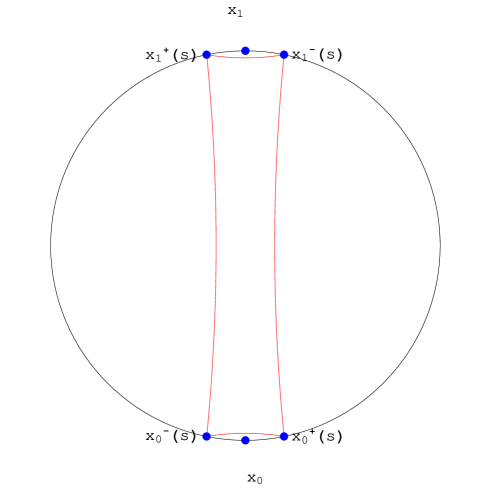
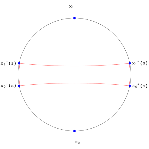
Figure 2: How does the length change?

Thus, there exist $s_{0}\in(0,L/2)$ so that

$$|A_{1}(s_{0})|+|A_{2}(s_{0})|=|B_{1}(s_{0})|+|B_{2}(s_{0})|.$$

So, given a fixed point $x_{0}\in\partial\mathcal{D}$, we have the existence of four distinct points $p_{1}=\alpha(s_{0})$, $p_{2}=\alpha(L/2-s_{0})$, $p_{3}=\alpha(L/2+s_{0})$ and $p_{4}=\alpha(-s_{0})$ ordered counter-clockwise so that

$$|A_{1}|+|A_{2}|=|B_{1}|+|B_{2}|,$$

where

$$B_{1} = \gamma(p_{1},p_{2})$$

$$A_{1} = \gamma(p_{2},p_{3})$$

$$B_{2} = \gamma(p_{3},p_{4})$$

$$A_{2} = \gamma(p_{4},p_{1}).$$

In analogy with the Euclidean case [3],

Definition 3.1.

Fix a point $x_{0}\in\partial\mathcal{D}$, let $p_{i}$, $i=1,\ldots,4$ be the points constructed above associated to $x_{0}\in\mathcal{D}$, then $\Gamma_{x_{0}}=A_{1}\cup B_{1}\cup A_{2}\cup A_{3}$ is called the quadrilateral associated to $x_{0}\in\mathcal{D}$ and it satisfies

$$|A_{1}|+|A_{2}|=|B_{1}|+|B_{2}|,$$

where

$$B_{1} = \gamma(p_{1},p_{2})$$

$$A_{1} = \gamma(p_{2},p_{3})$$

$$B_{2} = \gamma(p_{3},p_{4})$$

$$A_{2} = \gamma(p_{4},p_{1}).$$

Moreover, the interior domain $D_{x_{0}}$ bounded by $\Gamma_{x_{0}}$ is the square inscribed associated to $x_{0}\in\mathcal{D}$ (note that $D_{x_{0}}$ is a topological disc), and $B_{1}$ is called the bottom side (c.f. Figure 3).

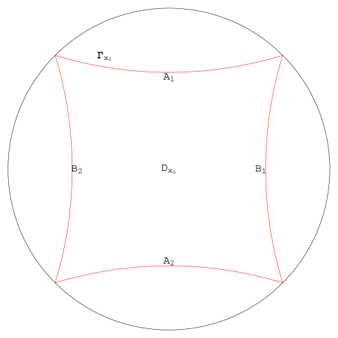
Figure 3: Scherk domain

Second, let us explain how to take the regular trapezoids: As above, fix $x_{0}\in\partial\mathcal{D}$ (from now on, $x_{0}$ will be fixed and we will omit it) and parametrize $\partial\mathcal{D}$ as $\alpha:\hbox{\bb R}/[0,L)\longrightarrow\partial\mathcal{D}$. Let $0\leq s_{1}<s_{2}<L$, or equivalently, two distinct and ordered points $p_{i}=\alpha(s_{i})\in\partial\mathcal{D}$, $i=1,2$. The aim is to construct a trapezoid in the region bounded by $\gamma(p_{1},p_{2})$ and $\alpha([s_{1},s_{2}])$. To do so, set $\bar{s}=\frac{s_{1}+s_{2}}{2}$, i.e., $\bar{p}=\alpha(\bar{s})$ is the mid-point. Define $\bar{p}^{\pm}(s)=\alpha(\bar{s}\pm s)$ for $0\leq s\leq\bar{s}$.

Set

$$l_{1}(s) = {\rm Length}\left(\gamma(p_{1},\bar{p}^{-}(s))\right)$$

$$l_{2}(s) = {\rm Length}\left(\gamma(\bar{p}^{-}(s),\bar{p}^{+}(s))\right)$$

$$l_{3}(s) = {\rm Length}\left(\gamma(\bar{p}^{+}(s),p_{2})\right)$$

$$l_{4}(s) = {\rm Length}\left(\gamma(p_{2},p_{1})\right).$$

Hence, for $s$ close to zero

$$l_{1}(s)+l_{3}(s)>l_{2}(s)+l_{4}(s)$$

by the Triangle Inequality, and for $s$ close to $\bar{s}$

$$l_{1}(s)+l_{3}(s)<l_{2}(s)+l_{4}(s),$$

since $l_{1}$ and $l_{3}$ go to zero and $l_{4}$ has positive length (c.f. Figure 4).

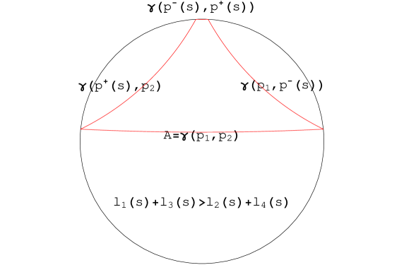
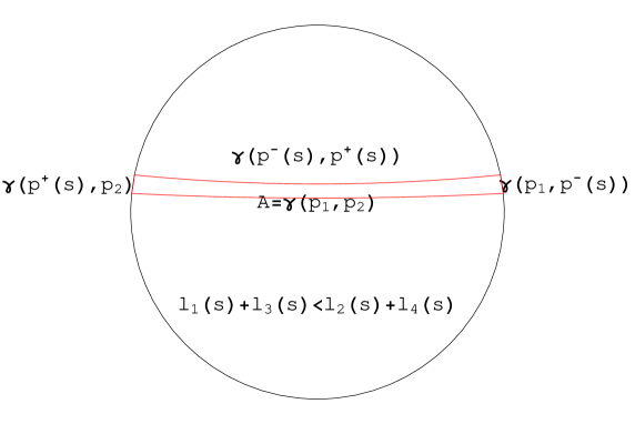
Figure 4: How does the trapezoid vary?

Thus, there exists $s_{0}\in(0,\bar{s})$ so that

$$l_{1}(s_{0})+l_{3}(s_{0})=l_{2}(s_{0})+l_{4}(s_{0}).$$

So, given a fixed point $x_{0}\in\partial\mathcal{D}$ and a geodesic arc $A:=\gamma(p_{1},p_{2})$ joining two (distinct and oriented) points in $\partial\mathcal{D}$, we have the existence of two distinct points $p^{-}=\alpha(\bar{s}-s_{0})$ and $p^{+}=\alpha(\bar{s}+s_{0})$ ordered count-clockwise so that

$$l_{1}+l_{3}=l_{2}+l_{4},$$

where

$$l_{1} = {\rm Length}\left(\gamma(p_{1},p^{-})\right)$$

$$l_{2} = {\rm Length}\left(\gamma(p^{-},p^{+})\right)$$

$$l_{3} = {\rm Length}\left(\gamma(p^{+},p_{2})\right)$$

$$l_{4} = {\rm Length}\left(\gamma(p_{2},p_{1})\right).$$

Moreover, the domain bounded by $\gamma(p_{1},p^{-})\cup\gamma(p^{-},p^{+})\cup\gamma(p^{+},p_{2})\cup\gamma(p_{1},p_{2})$ is a topological disc.

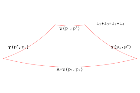
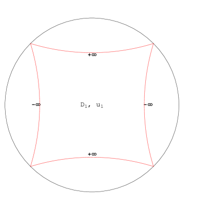
Figure 5: (Left) Regular Trapezoid

Figure 6: (Right) First Scherk domain

Again, in analogy with the Euclidean case,

Definition 3.2.

$E=\gamma(p_{1},p^{-})\cup\gamma(p^{-},p^{+})\cup\gamma(p^{+},p_{2})\cup\gamma(p_{1},p_{2})$ is called the regular trapezoid associated to the side $A$, here $A=\gamma(p_{1},p_{2})$ (and, of course, once we have fixed a point $x_{0}\in\partial\mathcal{D}$), and $p^{\pm}$ are given by the above construction (c.f. Figure 6).

Now, we can begin the example. We only highlight the main steps in the construction since, in essence, it is as in [3, Section III].

Fix $x_{0}\in\partial\mathcal{D}$ and let $D_{1}$ the inscribed quadrilateral associated to $x_{0}$ and $\Gamma_{1}=\partial D_{1}$ (see Definition 3.1). We label $A_{1},B_{1},A_{2},B_{2}$ the sides of $\Gamma_{1}$ ordered count-clockwise, with $B_{1}$ the bottom side. By construction, $D_{1}$ is a Scherk domain. One can check this fact using the Triangle Inequality. From Theorem 3.1, there is a minimal graph $u_{1}$ in $D_{1}$ which is $+\infty$ on the $A_{i}^{\prime}s$ sides and equals $-\infty$ on the $B_{i}^{\prime}s$ sides (c.f. Figure 6).

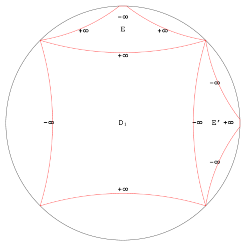
Figure 7: Attaching trapezoids

Henceforth, we will attach regular trapezoids (see Definition 3.2) to the sides of the quadrilateral $\Gamma_{1}$ in the following way. Let $E_{1}$ the regular trapezoid associated to the side $A_{1}$, and $E^{\prime}_{1}$ the regular trapezoid associated to the side $B_{1}$.

Consider the domain $D_{2}=D_{1}\cup E_{1}\cup E^{\prime}_{1}$, $\Gamma_{2}=\partial D_{2}$. This new domain does not satisfy the second condition of Theorem 3.1 ,we only have to consider the inscribed polygon $E$ (c.f. Figure 7).

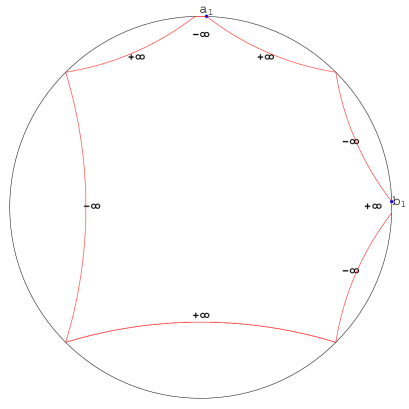
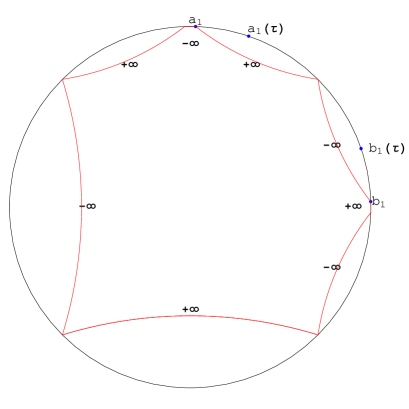
Figure 8: Moving the vertex of the trapezoid

So, the next step is to perturb $D_{2}$ in such a way that it becomes an admissible domain. Let $p$ be the common vertex of $E_{1}$ and $E^{\prime}_{1}$. Let $a_{1}$ the closed vertex of $E_{1}$ to $p$, and $b_{1}$ the closed vertex of $E^{\prime}_{1}$ to $p$ (c.f. Figure 8).

One moves the vertex $a_{1}$ towards $b_{1}$ to a nearby point $a_{1}(\tau)$ on $\partial\mathcal{D}$ (using the parametrization $\alpha:\hbox{\bb R}/[0,L)\longrightarrow\partial\mathcal{D}$ as we have been done throughout this Section). And then one moves $b_{1}$ towards $a_{1}$ to a nearby point $b_{1}(\tau)$ on $\partial\mathcal{D}$.

Let $\Gamma_{2}(\tau)$ the inscribed polygon obtained by this perturbation, $E_{1}(\tau)$ and $E^{\prime}_{1}(\tau)$ the perturbed regular trapezoids (c.f. Figure 9). Thus, for $\tau>0$ small, it is clear that:

• $\Gamma_{2}(\tau)$ satisfies Condition 1 in Theorem 3.1.

• $2a(E_{1}(\tau))<|E_{1}(\tau)|$ and $2b(E^{\prime}_{1}(\tau))<|E^{\prime}_{1}(\tau)|$.

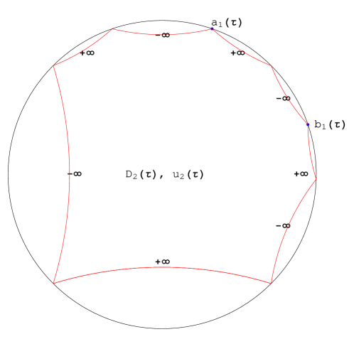
Figure 9: Perturbed Scherk domain

Now, we state the following Lemma that establish how we extend the Scherk surface in general.

Lemma 3.1.

Let $u$ be a Scherk graph on a polygonal domain $D_{1}=P(A_{1},B_{1},\ldots,A_{k},B_{k})$, where the $A_{i}^{\prime}s$ and $B_{i}^{\prime}s$ are the (geodesic) sides of $\partial D_{1}$ on which $u$ takes values $+\infty$ and $-\infty$ respectively. Let $K$ be a compact set in the interior of $D_{1}$. Let $D_{2}=P(E_{1},E^{\prime}_{1},A_{2},B_{2},\ldots,A_{k},B_{k})$ be the polygonal domain $D_{1}$ to which we attach two regular trapezoids $E_{1}$ to the side $A_{1}$ and $E^{\prime}_{1}$ to the side $B_{1}$. Let $E_{1}(\tau)$ and $E^{\prime}_{1}(\tau)$ be the perturbed polygons as above. Then for all $\epsilon>0$ there exists $\bar{\tau}>0$ so that, for all $0<\tau\leq\bar{\tau}$, $v$ is a Scherk graph on $P(E_{1}(\tau),E^{\prime}_{1}(\tau),A_{2},B_{2},\ldots,A_{k},B_{k})$ such that

$$\left\|u-v\right\|_{C^{2}(K)}\leq\epsilon.$$ (3.1)

Proof.

The proof of this Lemma relies on [3, Section IV] with the obvious differences that we need to use the results for Scherk graphs over a domain in a Hadamard surface stated in [9] and [5]. ∎

Before we return to the construction, let us explain how we construct a compact domain associated to any Scherk domain: Let $D=P(A_{1},B_{1},\ldots,A_{k},B_{k})$ be a Scherk domain in $\mathcal{D}$ with vertex $\left\{v_{1},\ldots,v_{2k}\right\}\in\partial\mathcal{D}$. Let $\beta_{v_{i}}:[0,1]\longrightarrow\overline{\mathcal{D}}$ denote the radial geodesic starting at $p_{0}\in\mathcal{D}$ (the center of the disc $\mathcal{D}$) and ending at $v_{i}\in\partial\mathcal{D}$. Note that any $\beta_{v_{i}}$ can not touch neither a $A_{i}$ side nor a $B_{i}$ side expect at the vertex.

Set $r<1$ and $p_{i}=\beta_{v_{i}}(r)\in\mathcal{D}$ for $i=1,\ldots,2k$. Consider the polygon

$$P=\bigcup_{i=1}^{2k-1}\gamma(p_{i},p_{i+i})\cup\gamma(p_{2k},p_{1})\subset D,$$

and let $K^{\prime}$ be the closure of the domain bounded by $P$, here $\gamma(p_{i},p_{i+1})$ is the geodesic arc joining $p_{i}$ and $p_{i+1}$ in $D$. Let $\mathcal{D}(p_{i},1-r)$ be geodesic disc centered at $p_{i}$ of radius $1-r$ for each $i=1,\ldots,2k$. Then,

Definition 3.3.

For $r<1$ close to $1$, the compact domain associated to the Scherk domain $D$ is given by

$$K=K^{\prime}\setminus\bigcup_{i=1}^{2k}\mathcal{D}(p_{i},1-r).$$

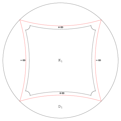
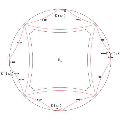
Figure 10: (Left) Compact domain associated to the inscribed quadrilateral

Figure 11: (Right) Attaching perturbed regular trapezoids

Now, we continue with the construction. Let $D_{1}=P(A_{1},B_{1},A_{2},B_{2})$ be the inscribed square in $\mathcal{D}$ (given in Definition 3.1), and the Scherk graph $u_{1}$ on $D_{1}$ which is $+\infty$ on the $A_{i}^{\prime}s$ sides and $-\infty$ on the $B_{i}^{\prime}s$ sides. Let $K_{1}$ be the compact domain associated to $D_{1}$ (see Definition 3.3). We choose $r_{1}<1$ close enough to one so that $u_{1}>1$ on the geodesic sides of $\partial K_{1}$ closer to the $A_{i}^{\prime}s$ sides and $u_{1}<-1$ on the geodesic sides of $\partial K_{1}$ closer to the $B_{i}^{\prime}s$ sides (cf. Figure 11).

Next, we attach perturbed regular trapezoids to the sides $A_{1}$ and $B_{1}$, so from Lemma 3.1, for any $\epsilon_{2}>0$ there exists $\tau_{2}>0$ so that $D_{2}(\tau)=D_{1}\cup E_{1}(\tau)\cup E^{\prime}_{1}(\tau)$ is a Scherk domain and $u_{2}(\tau)$, the Scherk graph defined on $D_{2}(\tau)$, satisfy

$$\left\|u_{1}-u_{2}(\tau)\right\|_{C^{2}(K_{1})}\leq\epsilon_{2},$$

for all $0<\tau\leq\tau_{2}$. Moreover, we can choose $u_{2}(\tau)$ so that $u_{1}(p_{0})=u_{2}(\tau)(p_{0})$ (here $p_{0}$ is the center of $\mathcal{D}$). Then, choose $\epsilon_{2}>0$ so that $u_{2}(\tau)>1$ on the geodesic sides of $\partial K_{1}$ closer to the $A_{i}^{\prime}s$ sides and $u_{2}(\tau)<-1$ on the geodesic sides of $\partial K_{1}$ closer to the $B_{i}^{\prime}s$ sides.

Let $K_{2}(\tau)$ be the compact domain associated to the Scherk domain $D_{2}(\tau)$. Choose $r_{2}<1$ close enough to one (in the definition of $K_{2}(\tau)$ given by Definition 3.3) so that, for $0<\tau\leq\tau_{2}$, $u_{2}(\tau)>2$ on those geodesic sides of $\partial K_{2}(\tau)$ parallel to the sides of $D_{2}(\tau)$ where $u_{2}(\tau)=+\infty$, and $u_{2}(\tau)<-2$ on the sides of $\partial K_{2}(\tau)$ parallel to sides of $D_{2}(\tau)$ where $u_{2}(\tau)=-\infty$ (cf. Figure 13).

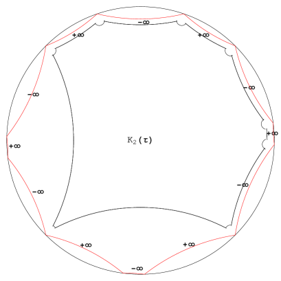
Figure 12: (Left) Compact domain associated to $D_{2}(\tau)$

Figure 13: (Right) Choosing $u_{3}(\tau)$

Continue by constructing the Scherk domain $D_{3}(\tau)$ by attaching perturbed regular trapezoids (as above) to the sides $A_{2}$ and $B_{2}$ of $D_{1}$. We know, for $\epsilon_{3}>0$, that there exist $\tau_{3}>0$ so that if $0<\tau\leq\tau_{3}$ then the Scherk graph $u_{3}(\tau)$ exists, $u_{3}(\tau)(p_{0})=u_{1}(p_{0})$ and

$$\left\|u_{3}(\tau)-u_{2}(\tau)\right\|_{C^{2}(K_{2}(\tau))}\leq\epsilon_{3}.$$

Moreover, choose $\epsilon_{3}>0$ so that $u_{3}(\tau)>3$ on the geodesic sides of $\partial K_{2}(\tau)$ closer to the $A_{i}^{\prime}s$ sides and $u_{3}(\tau)<-3$ on the geodesic sides of $\partial K_{2}(\tau)$ closer to the $B_{i}^{\prime}s$ sides (cf. Figure 13).

Now choose $\epsilon_{n}\longrightarrow 0$, $\tau_{n}\longrightarrow 0$, $K_{n}(\tau_{n})$ so that $K_{n}(\tau_{n})\subset K_{n+1}(\tau_{n+1})$, $\bigcup_{n}K_{n}(\tau_{n})=\mathcal{D}$. Then the $u_{n}(\tau_{n})$ converge to a graph $u$ on $\mathcal{D}$.

To see $u$ has the desired properties, we refer the reader to [3, pages 13 and 14] with the only difference that we need to use now Theorem 2.1.

Remark 3.1.

The above construction can be carried out in a more general situation. Actually, if we ask that

• The geodesic disc $\mathcal{D}$ has strictly convex boundary.

• There is a unique minimizing geodesic joining any two points of the disc.

Then, we can extend the above example.

References

- [1] L. Alías, M. Dajczer, H. Rosenberg, The Dirichlet problem for constant mean curvature surfaces in Heisenberg space, Calc. Var. Partial Differential Equations, 30 (2007), nº 4, 513–522. MR2332426.
- [2] P. Collin, H. Rosenberg, Construction of harmonic diffeomorphisms and minimal graphs. Preprint. Available at: arXiv:math.DG/0701547v1.
- [3] P. Collin, H. Rosenberg, Asymptotic values of minimal graphs ia disc. Preprint.
- [4] P. Fatou, Séries trigonométriques et séries de Taylor, Acta Math., 30 (1906), 335–400.
- [5] J.A. Gálvez, H. Rosenberg, Minimal surfaces and harmonic diffeomorphisms from the complex plane onto a Hadamard surface, preprint (math.DG/0807.0997).
- [6] L. Jorge, D. Koutroufiotis, An estimate for the curvature of bounded submanifolds, Amer. J. Math., 103 (1981), no. 4, 711–725. MR0623135.
- [7] C. Leandro, H. Rosenberg, Removable singularities for sections of Riemannian submersions of prescribed mean curvature. Preprint. Available at: http://people.math.jussieu.fr/ rosen/Singularity.pdf.
- [8] J. Nitsche, On new results in the theory of minimal surfaces, B. Amer. Math. Soc., 71 (1965), 195–270. MR0173993.
- [9] A.L. Pinheiro, A Jenkins-Serrin theorem in , To appear Bull. Braz. Math. Soc.