Theory of nonlinear optical response of ensembles of double quantum dots

Abstract

We study theoretically the time-resolved four-wave mixing (FWM) response of an ensemble of pairs of quantum dots undergoing radiative recombination. At short (picosecond) delay times, the response signal shows beats that may be dominated by the subensemble of resonant pairs, which gives access to the information of the inter-dot coupling. At longer delay times, the decay of the FWM signal is governed by two rates which result from the collective interaction between the two dots and the radiation modes. The two rates correspond to the subradiant and superradiant components in the radiative decay. Coupling between the dots enhances the collective effects and makes them observable even when the average energy mismatch between the dots is relatively large.

I Introduction

Double quantum dots (DQDs) are pairs of quantum dots (QDs) placed at a small distance from each other and coupled either by long-range dipole forces lovett03b ; danckwerts06 or by carrier tunneling through the inter-dot barrier bryant93 ; schliwa01 ; szafran01 (in the latter case, the system is referred to as a quantum dot molecule). Such systems attract much attention both in the theoretical and experimental research. This still growing interest is driven to a large extent by the technological promise these structures show for nanoelectronics and quantum information processing applications. A system built of two QDs can be viewed as a first step towards scalable semiconductor-based quantum devices. Coupling between the dots is essential here, as it allows one to induce conditional dynamics in the system and thus to realize the basic elements of quantum computing biolatti00 . Another interesting application of coupled QDs is generation of entangled photons gywat02 . It is therefore not surprising that much experimental work has been devoted to proving the existence of coupling in DQD systems ortner05 ; bayer01 ; ortner03 ; ortner05b ; krenner05b .

In this paper, we study the four-wave mixing (FWM) optical response of an inhomogeneous ensemble of self-assembled double quantum dots. The systems under consideration are QD pairs formed spontaneously by strain-induced nucleation, as is typical, e.g., in the InAs/GaAs system xie95 ; solomon96 (although, in fact, the exact arrangement of the QDs is not essential in our discussion). The FWM spectroscopy is an optical technique commonly used for extracting information on lifetimes and homogeneous dephasing from inhomogeneous ensembles borri99 ; borri01 ; vagov04 . It has been also applied to DQD ensembles borri03 , showing features that are clearly distinct from those observed in ensembles of individual QDs, like two-component decay and modified initial dephasing. As the physical properties of DQDs are much more complex than those of individual QDs it is not always possible to identify the mechanism responsible for these differences. In particular, it is not clear to which extent they may result from simple optical interference or quantum-optical mechanisms of collective radiative decay (sub- and superradiance), as opposed, e.g., to DQD-specific phonon-related dephasing channels, like dissipative exciton transfer govorov03 ; rozbicki08a .

Superradiance has been thoroughly studied for strongly excited atomic samples gross82 ; skribanovitz73 , where it is manifested as an outburst of radiation due to constructive interference of quantum-mechanical amplitudes for radiative transition in a massively correlated state of atoms interacting with a common radiation reservoir. Somewhat less spectacular form of this effect was also observed in QD ensembles scheibner07 where the radiative recombination was shown to increase for a sufficiently large number of dots. However, the essential features of the collective emission can be observed already in a two-emitter system: states with a delocalized excitation decay slower or faster, depending on the relative phase between the two components in the superposition (the first or the second emitter excited) agarwal74 ; sitek07a .

The goal of the present work is to identify the purely optical effects that may appear in the nonlinear optical response of an ensemble of DQDs. It has been pointed out that the dynamics of double dots coupled to a radiative reservoir is very reach, both in the open space sitek07a and in a cavity hughes05 . Here, we will show that the exponential decay of optical coherence, characteristic of a single QD, is replaced by a non-exponential, two-rate decay which may be related to sub- and superradiant components in the system evolution. As in the previously studied case of a single pair of nearly identical QDs sitek07a , the decay is strongly affected by the coupling between the dots. We show that the collective features in the radiative decay persist even for relatively large values of the energy mismatch between the dots (many orders of magnitude larger that the emission line width) as long as the coupling is of comparable magnitude. Another feature that emerges from our model is a damped oscillatory behavior of the FWM signal at short delays (sub-picosecond and picosecond time scales), which results from the optical interference of the signals emitted by various DQDs in the ensemble, dephased due to inhomogeneity of DQD parameters. As we will show, these beats may be dominated by a relatively long-living contribution from the minority subensemble of resonant DQDs (formed by dots with identical transition energies). In this way, the nonlinear response contains information on the coupling between the dots, irrespective of the energy mismatch between them.

The paper is organized as follows: In sec. II we present the system under consideration and define its model. Next, in sec. III we discuss the evolution of the system under two-pulse optical driving and derive the equations for the third order optical polarization. The results are discussed in sec. IV. Sec. V contains concluding remarks.

II The system

We study an ensemble of DQDs, each consisting of two QDs. The QDs in each pair are placed at a distance much smaller than the relevant photon wavelength so that spacial dependence of the electromagnetic (EM) field may be neglected (the Dicke limit). We assume that the polarization of the laser beam is chosen such that only one of the fundamental excitonic transitions in each dot is allowed. Each DQD can be then modelled as a four-level system with the basis states $|0\rangle\equiv|00\rangle$, $|1\rangle\equiv|01\rangle$, $|2\rangle\equiv|10\rangle$, $|3\rangle\equiv|11\rangle$, corresponding to the ground state (empty dots), an exciton in the second and first QD, and excitons in both QDs, respectively. A single DQD is composed of two QDs with energies $E_{1,2}=E\pm\Delta$. We will describe its evolution in a frame rotating with the frequency $E/\hbar$. Then, in the rotating wave approximation, the Hamiltonian for a single DQD is

$$H=H_{\mathrm{X}}+H_{\mathrm{L}}+H_{\mathrm{rad}}+H_{\mathrm{phot}}.$$

The first component describes the excitons

$$H_{X}=$$ (1)

$$\Delta\left(\hat{n}_{1}-\hat{n}_{2}\right)+V\left(\sigma^{\left(1\right)}_{-}\sigma^{\left(2\right)}_{+}+\sigma^{\left(1\right)}_{+}\sigma^{\left(2\right)}_{-}\right)+V_{B}\hat{n}_{1}\hat{n}_{2},$$

where $\sigma^{\left(j\right)}_{\pm}$ are creation and annihilation operators of an exciton in the j-th QD, $\hat{n}_{j}=\sigma_{+}^{(j)}\sigma_{-}^{(j)}$ is the occupation of the dot $j$, $V$ is the coupling between the dots (e.g., tunneling or Förster), and $V_{B}$ is a biexciton shift due to a static dipole interaction danckwerts06 .

The second term in the Hamiltonian accounts for the interaction with the laser field, which is treated classically,

$$H_{\mathrm{L}}=\frac{1}{2}\sum_{l}f_{l}(t)\left[e^{-i(\phi_{l}+Et_{l}/\hbar)}\left(\sigma^{\left(1\right)}_{-}+\sigma^{\left(2\right)}_{-}\right)+\mathrm{H.c.}\right],$$ (2)

where $f_{l}$, $\phi_{l}$, and $t_{l}$ are the amplitude envelopes, phases, and arrival times of the laser pulses, respectively.

The third term accounts for the interaction with the quantized EM field (radiation reservoir) in the dipole approximation.

$$H_{\mathrm{rad}}=\left(\sigma^{\left(1\right)}_{-}+\sigma^{\left(2\right)}_{-}\right)\sum_{\bm{k},\lambda}g_{\bm{k}\lambda}e^{i\left(\omega_{\bm{k}}-E/\hbar\right)t}b^{\dagger}_{\bm{k},\lambda}+\mathrm{H.c.},$$

where

$$g_{\bm{k}\lambda}=i\bm{d}\cdot\hat{e}_{\lambda}\left(\bm{k}\right)\sqrt{\frac{\hbar\omega_{\bm{k}}}{2\epsilon_{0}\epsilon_{r}v}},$$

$\bm{k}$ is a photon wave vector, $\omega_{\bm{k}}$ is the corresponding frequency, $\lambda$ denotes polarizations, $b_{\bm{k},\lambda},b_{\bm{k},\lambda}^{{\dagger}}$ are photon creation and annihilation operators, $\bm{d}$ is the interband dipole moment (for simplicity equal for all QDs), $\hat{e}_{\lambda}\left(\bm{k}\right)$ is a unit polarization vector, $\epsilon_{0}$ is the vacuum permittivity, $\epsilon_{\mathrm{r}}$ is the dielectric constant of the semiconductor, and $v$ is the normalization volume for the EM modes.

Finally,

$$H_{\mathrm{phot}}=\sum_{\bm{k},\lambda}\hbar\omega_{{\bm{k}}}b_{\bm{k},\lambda}^{{\dagger}}b_{\bm{k},\lambda}$$ (3)

is the Hamiltonian of the radiation reservoir.

To describe the ensemble of DQDs, we assume a Gaussian distribution function for the energies of the two dots,

$$g(E_{1},E_{2}) = \frac{1}{2\pi\sigma^{2}\sqrt{1-\rho^{2}}}$$ (4)

$$\times e^{-\frac{\left(E_{1}-\bar{E}_{1}\right)^{2}-2\rho\left(E_{1}-\bar{E}_{1}\right)\left(E_{2}-\bar{E}_{2}\right)+\left(E_{2}-\bar{E}_{2}\right)^{2}}{2\left(1-\rho^{2}\right)\sigma^{2}}}$$

with the mean transition energies $\bar{E}_{1}$, $\bar{E}_{2}$, identical energy variances $\sigma^{2}$ for both QDs, and a correlation coefficient $\rho$. Note that this distribution corresponds to an uncorrelated Gaussian distribution of the parameters $E$ and $\Delta$, $g\left(E,\Delta\right)=g_{E}\left(E\right)g_{\Delta}\left(\Delta\right)$, where

$$g_{A}\left(A\right)=\frac{1}{\sqrt{2\pi}\sigma_{A}}\exp\left[-\frac{\left(A-\overline{A}\right)^{2}}{2\sigma_{A}^{2}}\right],\quad A=E,\Delta,$$ (5)

with the mean values $\bar{E}=(\bar{E}_{1}+\bar{E}_{2})/2$ and $\bar{\Delta}=(\bar{E}_{1}-\bar{E}_{2})/2$ and variances $\sigma_{E}^{2}=\sigma^{2}(1+\rho)/2$ and $\sigma_{\Delta}^{2}=\sigma^{2}(1-\rho)/2$ (correlation between the QD energies $E_{1},E_{2}$ means less variance of their difference).

III The system evolution and FWM response

A FWM experiment, which we want to model, consists in exciting an ensemble of DQDs with two ultrashort laser pulses, arriving at $t_{1}=-\tau$ and $t_{2}=0$. The first step of the calculation is to find the optical polarization of a single DQD after the second pulse, which is proportional to

$$P(t)=\rho_{10}(t)+\rho_{20}(t)+\rho_{31}(t)+\rho_{32}(t)+\mathrm{c.c.},$$

where $t>0$, $\rho(t)$ is the density matrix of a DQD structure, and $\rho_{kl}=\langle k|\rho|l\rangle$. The first two terms are exciton coherences (polarizations) while the other two are referred to as biexciton polarizations. In order to extract the FWM polarization we pick out only the terms containing the phase factor $e^{i(2\phi_{2}-\phi_{1})}$, which mimics the frequency shifting and lock-in detection technique used in the actual experiment mecozzi96 ; borri99 . In the second step, the total optical response from the sample is obtained by summing up the contributions from individual DQDs with the weight factor $g(E,\Delta)$,

$$P_{\mathrm{FWM}}(t)=\int d\Delta dEg(E,\Delta)P(t).$$

III.1 Single DQD evolution

The detection of weak signals originating from the DQD ensemble is based on a heterodyne technique borri99 : The response $P_{\mathrm{FWM}}$ is superposed onto a reference pulse

$$E_{\mathrm{ref}}(t)=f_{\mathrm{ref}}(t-t_{0})e^{-i\overline{E}(t-t_{0})/\hbar}+\mathrm{c.c.},$$

arriving at a time $t_{0}$. We assume a Gaussian envelope

$$f_{\mathrm{ref}}(t)=\frac{1}{\sqrt{2\pi}\tau_{\mathrm{ref}}}\exp\left[-\frac{1}{2}\left(\frac{t}{\tau_{\mathrm{ref}}}\right)^{2}\right].$$

The measured signal is proportional to $|F(t_{0},\tau)|$, where

$$F(t_{0},\tau)=e^{i\overline{E}(t_{0}-\tau)/\hbar}\int dtP_{\mathrm{FWM}}^{(+)}(t)E_{\mathrm{ref}}^{(-)}(t),$$ (6)

where $P_{\mathrm{FWM}}^{(+)}$ and $E_{\mathrm{ref}}^{(-)}$ are the positive frequency part of the FWM signal and the negative frequency part of the reference pulse, respectively, and the (irrelevant) phase factor has been extracted for convenience.

We assume that the pulses are spectrally very broad to assure resonance with all the QDs in the ensemble. If the durations of the pulses are much shorter than both $\hbar/\Delta$ and $\hbar/V$, the action of each of them corresponds to an instantaneous, independent rotation of the state of each QD, that is, to the unitary transformation $\mathsf{U}_{l}=U_{l}\otimes U_{l}$, where

$$U_{l}=$$

$$\cos\left(\frac{\alpha_{l}}{2}\right)\mathbb{I}-i\sin\left(\frac{\alpha_{l}}{2}\right)\left[e^{-i(\phi_{l}+Et_{l}/\hbar)}|0\rangle\!\langle 1|+\mathrm{h.c.}\right].$$

Here $\mathbb{I}$ denotes the identity operator and

$$\alpha_{l}=\frac{1}{\hbar}\int_{-\infty}^{\infty}f_{l}(t)dt$$

is the pulse area.

We assume that the initial state of a DQD is $\rho(-\tau^{-})=|00\rangle\!\langle 00|$ ($t^{\pm}$ denotes just after or before a time instant $t$). The DQD is then excited with the first pulse. Just after this pulse, the system state is

$$\rho(-\tau^{+})=\mathsf{U_{1}}\rho(-\tau^{-})\mathsf{U^{\dagger}_{1}}$$ (7)

and the four matrix elements related to optical polarizations have the values

$$\rho_{01}(-\tau^{-}) = \rho_{02}(-\tau^{-})=\frac{i}{2}\sin\alpha_{1}\cos^{2}\frac{\alpha_{1}}{2}e^{-i\phi_{1}+iE\tau/\hbar},$$

$$\rho_{13}(-\tau^{-}) = \rho_{23}(-\tau^{-})=\frac{i}{2}\sin\alpha_{1}\sin^{2}\frac{\alpha_{1}}{2}e^{-i\phi_{1}+iE\tau/\hbar}.$$

From now on, we will only keep the terms which are of the first order in the first pulse area $\alpha_{1}$. In this approximation, the biexciton coherences do not contribute at this stage of the evolution.

Between the laser pulses, the evolution of the reduced density matrix of the charge subsystem is described by the Lindblad equation of the form sitek07a

$$\dot{\rho}=-\frac{i}{\hbar}[H_{\mathrm{X}},\rho]+\mathcal{L}[\rho],$$ (8)

with

$$\mathcal{L}[\rho]=\Gamma\left[\Sigma_{-}\rho\Sigma_{+}-\frac{1}{2}\{\Sigma_{+}\Sigma_{-},\rho\}_{+}\right],$$ (9)

where $\Gamma$ is the spontaneous decay rate for an individual dot and $\Sigma_{-}=\Sigma^{\dagger}_{+}=\sigma^{\left(1\right)}_{-}+\sigma^{\left(2\right)}_{-}$. This yields a closed system of four equations of motion for the negative frequency parts of optical polarizations,

$$\dot{\rho}_{01} = \left(i\Delta/\hbar-\Gamma/2\right)\rho_{01}+\left(iV/\hbar-\Gamma/2\right)\rho_{02}$$ (10a)

$$+\Gamma(\rho_{13}+\rho_{23}),$$

$$\dot{\rho}_{02} = \left(iV/\hbar-\Gamma/2\right)\rho_{01}-\left(i\Delta/\hbar+\Gamma/2\right)\rho_{02}$$ (10b)

$$+\Gamma(\rho_{13}+\rho_{23}),$$

$$\dot{\rho}_{23} = \left(iV_{\mathrm{B}}/\hbar+i\Delta/\hbar-3\Gamma/2\right)\rho_{23}$$ (10c)

$$-\left(iV/\hbar+\Gamma/2\right)\rho_{13},$$

$$\dot{\rho}_{13} = -\left(iV/\hbar+\Gamma/2\right)\rho_{23}$$ (10d)

$$+\left(iV_{\mathrm{B}}/\hbar-i\Delta/\hbar-3\Gamma/2\right)\rho_{13}.$$

The solution to these equation simplifies if one notes that for typical double dots the energy mismatch is much larger than the fundamental line width. Therefore, in the following we assume $\Gamma\ll\Omega/\hbar$, where $\Omega=(\Delta^{2}+V^{2})^{1/2}$ corresponds to the half-splitting of the single exciton states. This reflects the actual experimental situation as the energy mismatch observed in real samples ranges from a few meV to tens of meV gerardot03 ; gerardot05 ; borri03 while the recombination rate $1/\Gamma$ is typically of the order of 1 ns borri03 ; langbein04 ; gerardot05 .

Upon solving the equations (10a-d), one finds the exciton coherences at $t=0^{-}$,

$$\rho_{01(02)}(0^{-})=\frac{i}{4}\sin\alpha_{1}\cos^{2}\frac{\alpha_{1}}{2}e^{-i\phi_{1}+iE\tau/\hbar}$$

$$\times\left[\left(1-\frac{V\pm\Delta}{\Omega}\right)e^{\lambda_{0}\tau}+\left(1+\frac{V\pm\Delta}{\Omega}\right)e^{\lambda_{1}\tau}\right],$$

with

$$\lambda_{0(1)}=\mp i\frac{\Omega}{\hbar}-\frac{1}{2}\beta_{\mp}\Gamma,$$ (12)

where $\beta_{\pm}=1\pm V/\Omega$, and the upper sign corresponds to the first index or pair of indices.

The second pulse, with an area $\alpha_{2}$ arrives at $t=0$. In order to find the FWM response to the leading (third) order, we need to calculate the positive frequency parts of optical polarizations, keeping only terms of the second order, containing the phase factor $e^{2i\phi_{2}}$. Such terms depend only on the values of the negative frequency polarizations before the pulse and have the form

$$\rho_{10}(0^{+}) = \rho_{20}(0^{+})$$ (13a)

$$= \frac{e^{i\phi_{2}}}{4}\sin^{2}\alpha_{2}\left[\rho_{01}(0^{-})+\rho_{02}(0^{-})\right],$$

$$\rho_{31(32)}(0^{+}) = -\frac{e^{i\phi_{2}}}{4}\sin^{2}\alpha_{2}\rho_{02(01)}(0^{-}).$$ (13b)

Note that biexciton polarizations appear in the leading order and cannot be eliminated since, contrary to the single dot case, the transition to the molecular biexciton (excitons with the same polarization confined in different dots) is not forbidden by selection rules for any polarization of the laser beam.

The single exciton polarizations at an arbitrary time $t>0$ are found by using Eqs. (13a,b) as initial values for the system of equations of motion for positive frequency polarizations, which is obtained from Eqs. (10a-d) by complex conjugation. The total single-exciton polarization is $P^{(1)}(t)=\rho_{10}(t)+\rho_{20}(t)$ and is explicitly given by

$$P^{(1)}(t) = \frac{i}{8}\sin\alpha_{1}\cos^{2}\frac{\alpha_{1}}{2}\sin^{2}\alpha_{2}e^{i(2\phi_{2}-\phi_{1})}e^{iE\tau/\hbar}$$ (14)

$$\times\left(\beta_{-}e^{\lambda_{0}^{*}t}+\beta_{+}e^{\lambda_{1}^{*}t}\right)\left(\beta_{-}e^{\lambda_{0}\tau}+\beta_{+}e^{\lambda_{1}\tau}\right).$$

Although, in principle, the biexciton term affects the exciton coherences in the same order of the optical response (due to radiative recombination) one finds that the corresponding terms are of the order of $\hbar\Gamma/\Omega\ll 1$ and can be neglected.

For the biexciton polarizations, the evolution equations (10a-d) yield

$$\rho_{31(32)}=$$

$$\frac{1}{2}\left[\left(1\mp\frac{\Delta}{\Omega}\right)\rho_{31(32)}(0^{+})+\frac{V}{\Omega}\rho_{32(31)}(0^{+})\right]e^{\lambda_{2}^{*}t}$$

$$+\frac{1}{2}\left[\left(1\pm\frac{\Delta}{\Omega}\right)\rho_{31(32)}(0^{+})-\frac{V}{\Omega}\rho_{32(31)}(0^{+})\right]e^{\lambda_{3}^{*}t},$$

where

$$\lambda_{2(3)}=\mp i\Omega/\hbar+iV_{\mathrm{B}}/\hbar-\left(1+\frac{1}{2}\beta_{\pm}\right)\Gamma.$$ (15)

The biexciton contribution to the coherent polarization is then

$$P^{(2)}(t) = \rho_{31}+\rho_{32}$$ (16)

$$= \frac{i}{8}\sin\alpha_{1}\cos^{2}\frac{\alpha_{1}}{2}\sin^{2}\alpha_{2}e^{i(2\phi_{2}-\phi_{1})}e^{iE\tau/\hbar}$$

$$\times\left(\beta_{+}e^{\lambda_{2}^{*}t+\lambda_{1}\tau}+\beta_{-}e^{\lambda_{3}^{*}t+\lambda_{0}\tau}\right).$$

III.2 Ensemble response

The FWM polarization is obtained upon returning to the Schrödinger picture, which amounts to inserting the phase factor $e^{-iEt/\hbar}$ and adding up the contributions from all the dots in the ensemble according to their statistical distribution given by Eqs. (4) and (5). For the sake of the further discussion it is convenient to split the exciton contribution (14) into two parts and to write the total polarization as a sum of three contributions

$$P_{\mathrm{FWM}}(t)=$$ (17)

$$\frac{i}{8}\sin\left(\alpha_{1}\right)\cos^{2}\left(\frac{\alpha_{1}}{2}\right)\sin^{2}\left(\alpha_{2}\right)e^{-\frac{\Gamma}{2}\left(\tau+t\right)}$$

$$\times\int d\Delta dEg(E,\Delta)e^{-iE\left(t-\tau\right)/\hbar}\sum_{n=1}^{3}P_{n}(t,\Delta)+\mathrm{c.c.}$$

$$=\frac{i}{8}\sin\left(\alpha_{1}\right)\cos^{2}\left(\frac{\alpha_{1}}{2}\right)\sin^{2}\left(\alpha_{2}\right)$$

$$\times e^{-\frac{\sigma_{E}^{2}\left(t-\tau\right)^{2}}{2}-i\overline{E}\left(t-\tau\right)/\hbar-\frac{\Gamma}{2}\left(t+\tau\right)}$$

$$\times\int d\Delta g(\Delta)\sum_{n=1}^{3}P_{n}(t,\Delta)+\mathrm{c.c.},$$

where we inserted the definitions (12) and (15) into Eqs. (14) and (16) and defined

$$P_{n}(t,\Delta)=P_{n+}(t,\Delta)+P_{n-}(t,\Delta),$$

$$P_{1\pm}(t,\Delta)=\beta_{\pm}^{2}\exp\left[\mp\frac{V\Gamma}{2\Omega}\left(\tau+t\right)\pm i\Omega\left(\tau-t\right)/\hbar\right],$$

$$P_{2\pm}(t,\Delta)=\beta_{\pm}\beta_{-}\exp\left[\pm\frac{V\Gamma}{2\Omega}\left(\tau-t\right)\mp i\Omega\left(\tau+t\right)/\hbar\right],$$

$$P_{3\pm}(t,\Delta)=$$

$$-\beta_{\mp}\exp\left[-\left(\Gamma+iV_{B}/\hbar\right)t\pm\left(\frac{V\Gamma}{2\Omega}-i\Omega/\hbar\right)\left(\tau+t\right)\right].$$

The second form of Eq. (17) is obtained by performing the integration over $E$.

Next, one has to calculate the heterodyne signal generated by the FWM polarization overlapped with the reference signal, according to Eq. (6). The integration over time in Eq. (6) can easily be performed. Substituting Eq. (17) into Eq. (6) and performing some reasonable approximations, as discussed in detail in the Appendix, one finds

$$F(t_{0},\tau)=\sum_{n=1}^{3}F_{n}(t_{0},\tau),$$

where

$$F_{n}(t_{0},\tau) = \frac{i}{8}\sin\left(\alpha_{1}\right)\cos^{2}\left(\frac{\alpha_{1}}{2}\right)\sin^{2}\left(\alpha_{2}\right)$$ (18)

$$\times\int d\Delta g_{\Delta}(\Delta)[\mathcal{F}_{n+}(\Delta)+\mathcal{F}_{n-}(\Delta)].$$

Here

$$\mathcal{F}_{n\pm}(\Delta) = e^{i\overline{E}(t_{0}-\tau)/\hbar}\int dtP_{n\pm}^{(+)}(t,\Delta)E_{\mathrm{ref}}^{(-)}(t)$$ (19)

$$= \frac{1}{4\sqrt{1+\tau_{\mathrm{ref}}^{2}\sigma_{E}^{2}/\hbar}}\exp\left[-\frac{\sigma_{E}^{2}(t_{0}-\tau)^{2}}{2(\hbar^{2}+\tau_{\mathrm{ref}}^{2}\sigma_{E}^{2})}\right]$$

$$\times\exp\left[\mp i\frac{\Omega(t_{0}-\tau)}{\hbar(\hbar+\tau_{\mathrm{ref}}^{2}\sigma_{E}^{2}/\hbar)}\right]\Phi_{n\pm}(\Delta),$$

where

$$\Phi_{1\pm}(\Delta) = \beta^{2}_{\pm}\exp\left[-\frac{\Omega^{2}\tau^{2}_{\mathrm{ref}}}{2(\hbar^{2}+\tau_{\mathrm{ref}}^{2}\sigma_{E}^{2})}\right]$$ (20a)

$$\times\exp\left[-\beta_{\pm}\Gamma\tau\right],$$

$$\Phi_{2\pm}(\Delta) = \beta_{+}\beta_{-}\exp\left[-\frac{\Omega^{2}\tau^{2}_{\mathrm{ref}}}{2(\hbar^{2}+\tau_{\mathrm{ref}}^{2}\sigma_{E}^{2})}\right]$$ (20b)

$$\times\exp\left[\mp 2i\Omega\tau/\hbar\right]\exp\left[-\Gamma\tau\right],$$

$$\Phi_{3\pm}(\Delta) = -\beta_{\mp}\exp\left[-\frac{(\Omega\pm V_{\mathrm{B}})^{2}\tau^{2}_{\mathrm{ref}}}{2(\hbar^{2}+\tau_{\mathrm{ref}}^{2}\sigma_{E}^{2})}\right]$$ (20c)

$$\times\exp\left[-i(V_{\mathrm{B}}\pm 2\Omega)\tau/\hbar-\frac{iV_{\mathrm{B}}(t_{0}-\tau)}{(\hbar+\tau_{\mathrm{ref}}^{2}\sigma_{E}^{2}/\hbar)}\right]$$

$$\times\exp\left[-(1+\beta_{\mp})\Gamma\tau\right].$$

In order to calculate the time-resolved nonlinear response of the DQD ensemble, Eq. (19) must be integrated numerically with the distribution function $g_{\Delta}(\Delta)$, according to Eq. (18). Another integration, over $t_{0}$, yields the time-integrated (TI) FWM signal as a function of the delay time $\tau$, which is commonly used to characterize the dephasing in a physical system. The results will be discussed in the following section.

IV Results

In this section we present and discuss the time-resolved and time-integrated FWM response from an ensemble of double quantum dots, depending on the statistical distribution of the energy mismatch between the dots in the ensemble and on the strength of the coupling between the dots. We assume fixed values of the average energy mismatch $\bar{\Delta}=4$ meV, the standard deviation of the mean DQD transition energy $\sigma_{E}=8$ meV, the length of the reference pulse $\tau_{\mathrm{ref}}=21$ fs (corresponding to 50 fs full width at half maximum), and the spontaneous recombination rate for an individual dot $\Gamma=1$ ns^-1. We start by studying the nonlinear response for short (picosecond) delays; then we proceed to the discussion of the signal decay on long (nanosecond) time scales.

IV.1 FWM response for short delay times

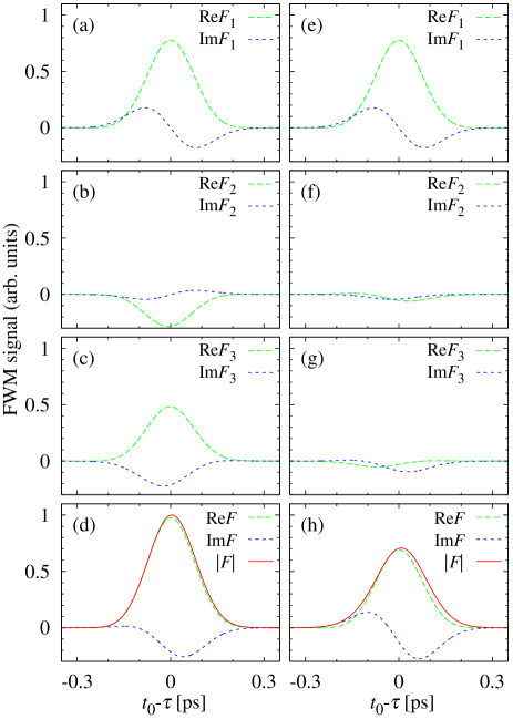
Figure 1: (Color online) (a-c) Real and imaginary parts (green dashed and blue dotted lines, respectively) of the three contributions $F_{n}(t_{0},\tau)$ to the FWM echo $F(t_{0},\tau)$ [Eqs. (18)–(20c)] for short delays, with $\tau=0.23$ ps, $V=2$ meV, $V_{\mathrm{B}}=1$ meV, $\sigma_{\Delta}=1$ meV. (e-g) As previously but at $\tau=0.61$ ps. (d,h) Real and imaginary parts of the total signal $F(t_{0},\tau)$, as well as its modulus, which corresponds to the measured signal, for the two values of $\tau$.

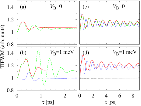
Figure 2: (Color online) (a,b) The evolution of the time-integrated signal for short delays without (a) and with (b) a biexciton shift for $\sigma_{\Delta}\ll\overline{\Delta}$ (no resonant dots in the ensemble). Red solid lines: $V=2$ meV, $\sigma_{\Delta}=1$ meV; green dashed lines: $V=2$ meV, $\sigma_{\Delta}=0.5$ meV; blue dotted lines: $V=0$ meV, $\sigma_{\Delta}=1$ meV. (c,d) As in (a) and (b), respectively, but for $\sigma_{\Delta}$ comparable with $\overline{\Delta}$. Red solid lines: $V=2$ meV, $\sigma_{\Delta}=3$ meV; green dashed line: $V=2$ meV, $\sigma_{\Delta}=5$ meV; blue dotted lines: $V=3$ meV, $\sigma_{\Delta}=3$ meV; grey dash dotted line $V=0$, $\sigma_{\Delta}=3$ meV.

It follows from Eq. (19) that all the contributions to the FWM signal are restricted to the short range of delay times around $t_{0}=\tau$, of width $\sim\hbar/\sigma_{\mathrm{E}}$, that is, they have the form of a photon echo. However, among the three contributions $F_{n}$ [Eq. (18)], the first one, $F_{1}$, has a different character than the other two. This results from the different structure of the phase factors of the form $e^{i\Omega\tau/\hbar}$ appearing in the last exponential term of Eq. (19), in the second exponential term of Eq. (20b) and in the second exponential term of Eq. (20c). Since $\Omega$ depends on $\Delta$, which varies across the ensemble, such terms tend to interfere destructively when the signal from different DQDs is added up. However, in the case of $F_{1}$, this phase term depends only on $t_{0}-\tau$, which is limited to the width $\hbar/\sigma_{\mathrm{E}}$ of the echo pulse. Therefore, the spread of the phase factors is also limited and independent of $\tau$. The only effect of this phase term is therefore a slight asymmetry of the echo pulse due to oscillations in $\operatorname{Im}F_{1}$, as shown in Fig. 1(a,e) (which makes it different from the simple pulse shape from an ensemble of individual dots). These oscillations are always in phase with the center of the echo peak, so that the peak area (that is, the time-integrated signal) is constant.

The situation is different in the case of the other two contributions $F_{2}$ and $F_{3}$. Here, another phase term appears, proportional to $\Omega\tau/\hbar$ or $(V_{\mathrm{B}}\pm 2\Omega)\tau/\hbar$ [in the second exponential terms of Eqs. (20b) and (20c)]. Thus, the phase of the signal at $t_{0}=\tau$ varies with $\tau$, which leads to a variation of the shape and magnitude of the echo. As can be seen by comparing Figs. 1(b,c)] with Figs. 1(f,g)], the contribution of these terms to the photon echo strongly depends on the delay $\tau$. As a result, also the amplitude of the total (actually measured) signal varies with time on picosecond time scales, as shown in Figs. 1(d,h). This variation leads to oscillations in the TI signal (Fig. 2). These oscillations are a manifestation of optical beats between the two dots. Their form depends on whether the ensemble contains a fraction of DQDs composed of identical (resonant) dots, that is, on the interplay of $\sigma_{\Delta}$ and $\overline{\Delta}$.

If $\sigma_{\Delta}\ll\overline{\Delta}$ then the signal originates from all the DQDs, whose values of the energy mismatch $\Delta$ lie roughly within $\sigma_{\Delta}$ from $\overline{\Delta}$. The inhomogeneity of the values of $\Delta$ translates into inhomogeneity of $\Omega$ and leads to a spread of phases in the terms like $\exp(i\Omega\tau)/\hbar$, which increases as $\tau$ increases. Since the total signal from the sample is a coherent sum of the fields emitted by all DQDs, this phase distribution leads to quenching of the two contributions $F_{2}$ and $F_{3}$ at $\tau\sim\hbar\Omega/(\Delta\sigma_{\mathrm{\Delta}})\ll 1/\Gamma$ and, therefore, to vanishing of the oscillations. This can be clearly seen in Fig. 2(a,c). This effect is due to the fact that the probe pulse acts symmetrically on both dots and, therefore, can invert (refocus) only the dephasing due to the inhomogeneous distribution of the average transition energies but not that resulting from the inhomogeneity of the energy mismatch between the dots in a single pair.

The evolution of the optical signal becomes more interesting if $\sigma_{\Delta}\gtrsim\overline{\Delta}$. This condition means that the ensemble contains a fraction of resonant DQDs, that is, such that have nearly identical transition energies. The frequency $\Omega$ has a minimum at $\Delta=0$ which corresponds to a stationary point of the phase distribution over the ensemble. Therefore, all the nearly resonant QDs emit radiation in phase and can dominate the contributions $F_{2}$ and $F_{3}$ of the ensemble when the signal from the possibly much more numerous dots with $\Delta\sim\overline{\Delta}$ has dephased as described above. An essential point is that, since this minority resonant subensemble has $\Delta\sim 0$, the frequency of the beats is very close to $2V/\hbar$ or $(2V-V_{\mathrm{B}})/\hbar$ [note that the term with this frequency has a much larger amplitude in Eq. (20c) than that with the frequency $(2V+V_{\mathrm{B}})/\hbar$ since for $\Delta\to 0$ one has $\beta_{-}\to 0$]. In this way, the nonlinear response gives a direct access to the values of the inter-dot couplings and to the properties of resonant dots, even if they are a minority in the ensemble. The beats originating from the resonant subensemble show slower damping than those from the majority DQDs but still they vanish on the time scales of several picoseconds.

IV.2 FWM response for long delays

For longer delays, only $F_{1}$ contributes to the signal. Out of the two components making up this term, $F_{1+}$ has the decay rate $\Gamma_{+}=\beta_{+}\Gamma>\Gamma$. This is the superradiant component of the optical coherence, the decay rate of which reaches $2\Gamma$ when $V\gg\Delta$. The other, subradiant component $F_{1-}$ has the decay rate $\Gamma_{-}=\beta_{-}\Gamma<\Gamma$, which vanishes in the limit of strongly coupled dots. The relative amplitude of these two components is $\beta_{+}/\beta_{-}$, so that the superradiant one dominates if the coupling is strong, with a subradiant tail visible only at long delays.

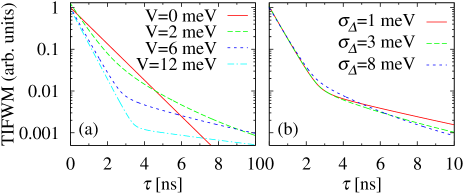
Figure 3: (Color online) Time-integrated FWM response. (a) Dependence on the coupling strength $V$ for $\sigma_{\Delta}=3$ meV. (b) Dependence on the inhomogeneity of the energy mismatch for $V=5$ meV.

The decay of the FWM signal at long delay times is shown in Fig. 3(a) for different strengths of coupling between the dots. For $V=0$, both decay rates are equal to $\Gamma$ and one observes a usual exponential decay. As the coupling increases, the decay of the FWM response becomes non-exponential due to the presence of the sub- and superradiant components. For $V\sim\Delta$, the decay sets off with an intermediate rate between $\Gamma$ and $2\Gamma$ but it deviates from an exponential form rather quickly. When $V\gg\Delta$ the FWM response is almost completely dominated by the superradiant component, showing an exponential decay with the rate $2\Gamma$ over a very long time range, with only a weak tail corresponding to the subradiant part of the signal.

Since the decay rates $\Gamma_{\pm}$ depend on $V/\Omega=V/(V^{2}+\Delta^{2})^{1/2}$, which varies over the ensemble due to the inhomogeneity of $\Delta$, they change from one DQD to another. In order to see how this inhomogeneity effect influences the nonlinear optical response we plot the time-integrated FWM response for a few values of $\sigma_{\Delta}$ in Fig. 3(b). The influence of this parameter is rather small and appears only for rather long times. The major effect is some softening of the shoulder which marks the transition from the dominating superradiant contribution to the subradiant tail. However, this happens only when $\sigma_{\Delta}\gg\Omega$.

Interestingly, as long as only the leading order response is considered, the biexciton shift appears only in the short-living term $F_{3}$. At longer times, this kind of coupling does not affect the FWM response at all. Thus, there are no beats from molecular biexcitons in the FWM response.

V Conclusion

Our results show that the shape and decay rate of the time-resolved FWM signal provide rich information on the properties of the DQDs in the ensemble, including coupling between the QDs. In the time-integrated signal for long delay times, one observes a transition from the regime of independent decay (with the usual decay rate) to superradiant decay (double rate) via intermediate cases of non-exponential decay. This transition is driven by the interplay of the energy mismatch between the QDs forming the DQD system and the coupling between them and is only weakly affected by the distribution of the energy mismatch. The superradiance effect observed in the decay of the FWM response is strongly stabilized by the coupling between the dots and can survive even when the energy mismatch is many orders of magnitude larger than the radiative line width.

Unlike ensembles of individual QDs, the DQD samples show interesting and meaningful features also in the TI signal at short delays (several picoseconds). In this range of delay times, the signal has the form of oscillations which result from optical beats between the radiation emitted from different DQDs. The form and decay time of these oscillations depends on the presence of a resonant subensemble (a subset of DQDs with matched transition energies) in the inhomogeneous ensemble. If such subensemble is present, its contribution dominates the short-delay response yielding a direct access to the strength of interaction between the dots forming the DQDs.

In our study, we assumed that the surface density of DQDs in the ensemble is not very high and the distribution of the transition energies is rather broad so that collective effects on the level of the ensemble are absent. Including such effects would require applying a more general theory milonni74 ; milonni75 ; slepyan01 , as the DQDs are spaced by distances comparable or larger than the emitted wave length so that propagation and retardation effects would come into play.

Appendix A Third order response: approximations

In this Appendix we give the full formulas for the components of the third order response and present the details of the approximations that lead to Eqs. (20a-c). Substituting Eq. (17) into Eq. (6) one finds the FWM response signal in the form of Eqs. (18) and (19), with

$$\Phi_{1\pm}(\Delta) = \beta^{2}_{\pm}\exp\left[\frac{(2i\Omega/\hbar\pm\beta_{\pm}\Gamma)^{2}\tau^{2}_{\mathrm{ref}}}{8(1+\tau_{\mathrm{ref}}^{2}\sigma_{E}^{2}/\hbar^{2})}\right]$$ (21a)

$$\times\exp\left[-\beta_{\pm}\Gamma\tau-\frac{\beta_{\pm}\Gamma(t_{0}-\tau)}{2(1+\tau_{\mathrm{ref}}^{2}\sigma_{E}^{2}/\hbar^{2})}\right],$$

$$\Phi_{2\pm}(\Delta) = \beta_{+}\beta_{-}\exp\left[\frac{(2i\Omega/\hbar\pm\beta_{\pm}\Gamma)^{2}\tau^{2}_{\mathrm{ref}}}{8(1+\tau_{\mathrm{ref}}^{2}\sigma_{E}^{2}/\hbar^{2})}\right]$$ (21b)

$$\times\exp\left[\mp 2i\Omega/\hbar\tau\right]$$

$$\times\exp\left[-\Gamma\tau-\frac{\beta_{\pm}\Gamma(t_{0}-\tau)}{2(1+\tau_{\mathrm{ref}}^{2}\sigma_{E}^{2}/\hbar^{2})}\right],$$

$$\Phi_{3\pm}(\Delta) = -\beta_{\mp}\exp\left[\frac{(2i\Omega/\hbar\pm\left(2+\beta_{\mp}\right)\Gamma)^{2}\tau^{2}_{\mathrm{ref}}}{8(1+\tau_{\mathrm{ref}}^{2}\sigma_{E}^{2}/\hbar^{2})}\right]$$ (21c)

$$\times\exp\left[-\frac{\tau_{\mathrm{ref}}^{2}V_{B}(V_{B}\pm 2\Omega)}{2(\hbar^{2}+\tau_{\mathrm{ref}}^{2}\sigma_{E}^{2})}\right]$$

$$\times\exp\left[i\frac{(2+\beta_{\mp})\Gamma\tau_{\mathrm{ref}}^{2}V_{B}}{2(\hbar+\tau_{\mathrm{ref}}^{2}\sigma_{E}^{2}/\hbar)}\right]$$

$$\times\exp\left[-i(V_{\mathrm{B}}\pm 2\Omega)\tau/\hbar-\frac{iV_{\mathrm{B}}(t_{0}-\tau)}{\hbar+\tau_{\mathrm{ref}}^{2}\sigma_{E}^{2}/\hbar}\right]$$

$$\times\exp\left[-(1+\beta_{\mp})\Gamma\tau-\frac{(2+\beta_{\mp})\Gamma(t_{0}-\tau)}{2(1+\tau_{\mathrm{ref}}^{2}\sigma_{E}^{2}/\hbar^{2})}\right].$$

The values of the radiative decay rate $\Gamma$ and the inhomogeneous ensemble broadening of the transition energies $\sigma_{\mathrm{E}}$ are of the order of $\mu$eV and tens of meVs, respectively, while the typical duration of a reference pulse is about 100 fs or less. Based on these values, Eqs. (21a-c) can be considerably simplified.

In the first exponents in Eqs. (21a,b), one can write (consistently with the approximation $\Gamma\ll\Omega/\hbar$ used throughout this paper)

$$(2i\Omega/\hbar\pm\beta_{\pm}\Gamma)^{2}\tau^{2}_{\mathrm{ref}}\approx-4\Omega^{2}\tau^{2}/\hbar^{2}\pm 4i\beta_{\pm}\Gamma\tau^{2}_{\mathrm{ref}}.$$

Moreover, typically $\Gamma\tau_{\mathrm{ref}}\sim 10^{-4}$ and $\Omega\tau_{\mathrm{ref}}/\hbar\sim 0.1$, hence the imaginary part can be safely neglected. The same argument holds for the first exponential term in Eq. (21c), so that in all three exponents this term can be replaced by $\exp[-(1/2)\Omega^{2}/(\hbar^{2}+\tau_{\mathrm{ref}}^{2}\sigma_{E}^{2})]$.

Because of the Gaussian term in Eq. (19), it is clear that the measured signal is of considerable magnitude only when $|t_{0}-\tau|\lesssim\hbar/\sigma_{E}$, which reflects the ‘photon echo’ nature of the FWM response. Since $\hbar\Gamma/\sigma_{\mathrm{E}}\ll 1$, the very last terms in Eqs. (21a-c), proportional to $\Gamma(t_{0}-\tau)$, can be discarded. The third exponential term in Eq. (21c) is also negligible, as $\tau_{\mathrm{ref}}\Gamma\ll 1$, while $\tau_{\mathrm{ref}}V_{\mathrm{B}}/\hbar$ is typically of the order of 0.1 (for a biexciton shift of a few meV). With these approximations one arrives at the Eqs. (20a-c).

References

- (1) B. W. Lovett, J. H. Reina, A. Nazir, and G. A. D. Briggs, Phys. Rev. B 68, 205319 (2003).
- (2) J. Danckwerts, K. J. Ahn, J. Förstner, and A. Knorr, Phys. Rev. B 73, 165318 (2006).
- (3) G. W. Bryant, Phys. Rev. B 47, 1683 (1993).
- (4) A. Schliwa, O. Stier, R. Heitz, M. Grundmann, and D. Bimberg, Phys. Stat. Sol. (b) 224, 405 (2001).
- (5) B. Szafran, S. Bednarek, and J. Adamowski, Phys. Rev. B 64, 125301 (2001).
- (6) E. Biolatti, R. C. Iotti, P. Zanardi, and F. Rossi, Phys. Rev. Lett. 85, 5647 (2000).
- (7) O. Gywat, G. Burkard, and D. Loss, Phys. Rev. B 65, 205329 (2002).
- (8) G. Ortner, I. Yugova, G. Baldassarri Höger von Högersthal, A. Larionov, H. Kurtze, D. R. Yakovlev, M. Bayer, S. Fafard, Z. Wasilewski, P. Hawrylak, Y. B. Lyanda-Geller, T. L. Reinecke, A. Babinski, M. Potemski, V. B. Timofeev, and A. Forchel, Phys. Rev. B 71, 125335 (2005).
- (9) M. Bayer, P. Hawrylak, K. Hinzer, S. Fafard, M. Korkusinski, Z. R. Wasilewski, O. Stern, and A. Forchel, Science 291, 451 (2001).
- (10) G. Ortner, M. Bayer, A. Larionov, V. B. Timofeev, A. Forchel, Y. B. Lyanda-Geller, T. L. Reinecke, P. Hawrylak, S. Fafard, and Z. Wasilewski, Phys. Rev. Lett. 90, 086404 (2003).
- (11) G. Ortner, M. Bayer, Y. Lyanda-Geller, T. L. Reinecke, A. Kress, J. P. Reithmaier, and A. Forchel, Phys. Rev. Lett. 94, 157401 (2005).
- (12) H. J. Krenner, M. Sabathil, E. C. Clark, A. Kress, D. Schuh, M. Bichler, G. Abstreiter, and J. J. Finley, Phys. Rev. Lett. 94, 057402 (2005).
- (13) Q. Xie, A. Madhukar, P. Chen, and N. P. Kobayashi, Phys. Rev. Lett. 75, 2542 (1995).
- (14) G. S. Solomon, J. A. Trezza, A. F. Marshall, and J. S. Harris, Jr., Phys. Rev. Lett. 76, 952 (1996).
- (15) P. Borri, W. Langbein, J. Mørk, J. M. Hvam, F. Heinrichsdorff, M.-H. Mao, and D. Bimberg, Phys. Rev. B 60, 7784 (1999).
- (16) P. Borri, W. Langbein, S. Schneider, U. Woggon, R. L. Sellin, D. Ouyang, and D. Bimberg, Phys. Rev. Lett. 87, 157401 (2001).
- (17) A. Vagov, V. M. Axt, T. Kuhn, W. Langbein, P. Borri, and U. Woggon, Phys. Rev. B 70, 201305(R) (2004).
- (18) P. Borri, W. Langbein, U. Woggon, M. Schwab, M. Bayer, S. Fafard, Z. Wasilewski, and P. Hawrylak, Phys. Rev. Lett. 91, 267401 (2003).
- (19) A. O. Govorov, Phys. Rev. B 68, 075315 (2003).
- (20) E. Rozbicki and P. Machnikowski, Phys. Rev. Lett. 100, 027401 (2008).
- (21) M. Gross and S. Haroche, Phys. Rep. 93, 301 (1982).
- (22) N. Skribanowitz, I. P. Herman, J. C. MacGilvray, and M. S. Feld, Phys. Rev. Lett. 30, 309 (1973).
- (23) M. Scheibner, T. Schmidt, L. Worschech, A. Forchel, G. Bacher, T. Passow, and D. Hommel, Nature Physics 3, 106 (2007).
- (24) A. Sitek and P. Machnikowski, Phys. Rev. B 75, 035328 (2007).
- (25) G. S. Agarwal, Quantum Statistical Theories of Spontaneous Emission and their Relation to Other Approaches, Vol. 70 of Springer tracts in modern physics, G. Höhler (Ed.) (Springer, Berlin, 1974).
- (26) S. Hughes, Phys. Rev. Lett. 94, 227402 (2005).
- (27) A. Mecozzi, J. Mørk, and M. Hofmann, Opt. Lett. 21, 1017 (1996).
- (28) B. Gerardot, I. Shtrichman, D. Hebert, and P. Petroff, J. Cryst. Growth 252, 44 (2003).
- (29) B. D. Gerardot, S. Strauf, M. J. A. de Dood, A. M. Bychkov, A. Badolato, K. Hennessy, E. L. Hu, D. Bouwmeester, and P. M. Petroff, Phys. Rev. Lett. 95, 137403 (2005).
- (30) W. Langbein, P. Borri, U. Woggon, V. Stavarache, D. Reuter, and A. D. Wieck, Phys. Rev. B 70, 033301 (2004).
- (31) P. W. Milonni and P. L. Knight, Phys. Rev. A 10, 1096 (1974).
- (32) P. W. Milonni and P. L. Knight, Phys. Rev. A 11, 1090 (1975).
- (33) G. Y. Slepyan, S. A. Maksimenko, V. P. Kalosha, A. Hoffmann, and D. Bimberg, Phys. Rev. B 64, 125326 (2001).