Chaotic response of global climate to long-term solar forcing variability

Abstract

It is shown that global climate exhibits chaotic response to solar forcing variability in a vast range of timescales: from annual to multi-millennium. Unlike linear systems, where periodic forcing leads to periodic response, nonlinear chaotic response to periodic forcing can result in exponentially decaying broad-band power spectrum with decay rate $T_{e}$ equal to the period of the forcing. It is shown that power spectrum of a reconstructed time series of Northern Hemisphere temperature anomaly for the past 2,000 years has an exponentially decaying broad-band part with $T_{e}\simeq 11$ yr, i.e. the observed decay rate $T_{e}$ equals the mean period of the solar activity. It is also shown that power spectrum of a reconstruction of atmospheric $CO_{2}$ time fluctuations for the past 650,000 years, has an exponentially decaying broad-band part with $T_{e}\simeq 41,000$ years, i.e. the observed decay rate $T_{e}$ equals the period of the obliquity periodic forcing. A possibility of a chaotic solar forcing of the climate has been also discussed. These results clarify role of solar forcing variability in long-term global climate dynamics (in particular in the unsolved problem of the glaciation cycles) and help in construction of adequate dynamic models of the global climate.

I Introduction

Behavior of a chaotic system can be significantly altered by applying of a periodic forcing. Already pioneering studies of the effect of external periodic forcing on the first Lorenz model of the chaotic climate revealed very interesting properties of chaotic response (see, for instance, golub ,ahlers ,fran ). The forcing does not always have the result that one might expect bg ,chab ,tam . The climate, where the chaotic behavior was discovered for the first time, is still one of the most challenging areas for the chaotic response theory. One should discriminate between chaotic weather (time scales up to several weeks) and a more long-term climate variation. The weather chaotic behavior usually can be directly related to chaotic convection, while appearance of the chaotic properties for the long-term climate events is a non-trivial and challenging phenomenon. It seems that such properties can play a significant role even for glaciation cycles, i.e. at least at multi-millennium time scales hC ,sal . Cyclic forcing, due to astronomical modulations of the solar input, rightfully plays a central role in the long-term climate models. Paradoxically, it is a very non-trivial task to find imprints of this forcing in the long-term climate data. It will be shown in present paper that just unusual properties of chaotic response are the main source of this problem.

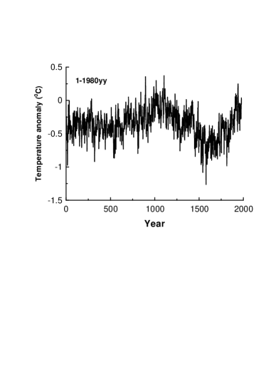
Figure 1: A reconstruction of Northern Hemisphere temperature anomaly for the past 2,000 years.

II Global temperature response to periodic solar forcing

Figure 1 shows a reconstruction of Northern Hemisphere temperatures for the past 2,000 years (the data for this figure were taken from Ref. paleoT ). This multi-proxy reconstruction was performed by the authors of Ref. moberg using combination of low-resolution proxies (lake and ocean sediments) with comparatively high-resolution tree-ring data. Figure 2 shows a power spectrum of the data set calculated using the maximum entropy method, because it provides an optimal spectral resolution even for small data sets. The spectrum exhibits a wide peak indicating a periodic component with a period around 22 y, and a broad-band part with exponential decay:

$$E(f)\sim e^{-f/f_{e}}$$

A semi-logarithmic plot was used in Fig. 2 in order to show the exponential decay more clearly (at this plot the exponential decay corresponds to a straight line). Both stochastic and deterministic processes can result in the broad-band part of the spectrum, but the decay in the spectral power is different for the two cases. The exponential decay indicates that the broad-band spectrum for these data arises from a deterministic rather than a stochastic process. For a wide class of deterministic systems a broad-band spectrum with exponential decay is a generic feature of their chaotic solutions Refs. o -hav .

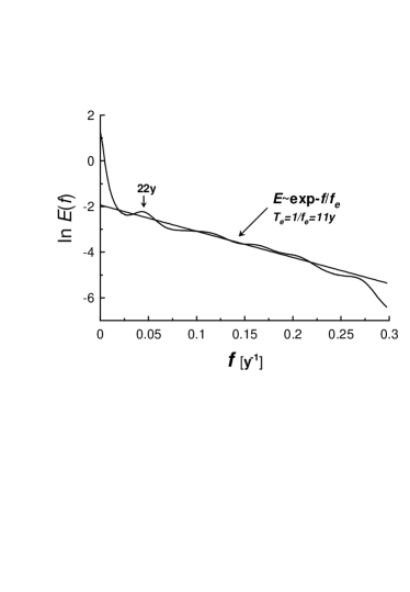
Figure 2: Spectrum of the data, shown in Fig. 1, in semi-logarithmic scales. The straight line indicates the exponential decay Eq. (1).

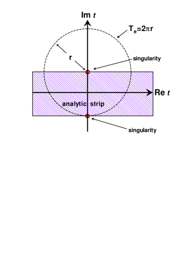
Figure 3: A sketch of the complex time plane for the parametric modulation with period $T_{e}$.

Nature of the exponential decay of the power spectra of the chaotic systems is still an unsolved mathematical problem. A progress in solution of this problem has been achieved by the use of the analytical continuation of the equations in the complex domain (see, for instance, fm ). In this approach the exponential decay of chaotic spectrum is related to a singularity in the plane of complex time, which lies nearest to the real axis. Distance between this singularity and the real axis determines the rate of the exponential decay. For many interesting cases chaotic solutions are analytic in a finite strip around the real time axis. This takes place, for instance for attractors bounded in the real domain (the Lorentz attractor, for instance). In this case the radius of convergence of the Taylor series is also bounded (uniformly) at any real time. If parameters of the dynamical system fluctuate periodically around their mean values with period $T_{e}$, then the restriction of the Taylor series convergence (at certain conditions) is determined by the period of the parametric modulation, and the width of the analytic strip around real time axis equals $T_{e}/2\pi$ (cf. Fig. 4). Let us consider, for simplicity, solution $u(t)$ with simple poles only, and to define the Fourier transform as follows

$$u(\omega)=(2\pi)^{-1/2}\int_{-T_{e}/2}^{T_{e}/2}dt~{}e^{-i\omega t}u(t)$$

Then using the theorem of residues

$$u(\omega)=i(2\pi)^{1/2}\sum_{j}R_{j}\exp(i\omega x_{j}-|\omega y_{j}|)$$

where $R_{j}$ are the poles residue and $x_{j}+iy_{j}$ are their location in the relevant half plane, one obtains asymptotic behavior of the spectrum $E(\omega)=|u(\omega)|^{2}$ at large $\omega$

$$E(\omega)\sim\exp(-2|\omega y_{min}|)$$

where $y_{min}$ is the imaginary part of the location of the pole which lies nearest to the real axis. Therefore, exponential decay rate of the broad-band part of the system spectrum, Eq. (1), equals the period of the parametric forcing.

The chaotic spectrum provides two different characteristic time-scales for the system: a period corresponding to fundamental frequency of the system, $T_{fun}$, and a period corresponding to the exponential decay rate, $T_{e}=1/f_{e}$ (cf. Eq. (1)). The fundamental period $T_{fun}$ can be estimated using position of the low-frequency peak, while the exponential decay rate period $T_{e}=1/f_{e}$ can be estimated using the slope of the straight line of the broad-band part of the spectrum in the semi-logarithmic representation (Fig. 2). From Fig. 2 we obtain $T_{fun}\simeq 22\pm 2$y and $T_{e}\simeq 11\pm 1y$ (the estimated errors are statistical ones). Thus, the solar activity period of 11 years is really a dominating factor in the chaotic temperature fluctuations at the annual time scales, although it is hidden for linear interpretation of the power spectrum. In the nonlinear interpretation the additional period $T_{fun}\simeq 22y$ might correspond to the fundamental frequency of the underlying nonlinear dynamical system. It is surprising that this period is close to the 22y period of the Sun’s magnetic poles polarity switching. It should be noted that the authors of Ref. mu found a persistent 22y cyclicity in sunspot activity, presumably related to interaction between the 22y period of magnetic poles polarity switching and a relic solar (dipole) magnetic field. Therefore, one cannot rule out a possibility that the broad peak, in a vicinity of frequency corresponding to the 22y period, is a quasi-linear response of the global temperature to the weak periodic modulation by the 22y cyclicity in sunspot activity. I.e. strong enough periodic forcing results in the non-linear (chaotic) response whereas a weak periodic component of the forcing can result in a quasi-linear (periodic) response.

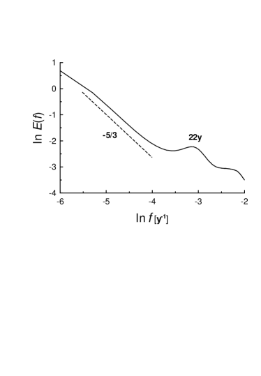
Figure 4: Spectrum of the data, shown in Fig. 1, in ln-ln scales. The dashed straight line indicates the Kolmogorov-like spectrum: $E(f)\sim f^{-5/3}$. The high-frequency part has been cut in order to show the low-frequency part.

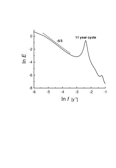
Figure 5: Spectrum of the galactic cosmic ray count rate fluctuations in the ln-ln scales. The straight dashed line is drawn to indicate the Kolmogorov scaling law $E(f)\sim f^{(-5/3)}$.

Figure 4 shows the same power spectrum as in Fig. 2 but in ln-ln scales. A dashed straight line in this figure indicates a scaling with ’-5/3’ exponent: $E(f)\sim f^{-5/3}$. Although, the scaling interval is short, the value of the exponent is rather intriguing. This exponent is well known in the theory of fluid (plasma) turbulence and corresponds to so-called Kolmogorov’s cascade process. This process is very universal for turbulent fluids and plasmas gibson ,clv . For turbulent processes on Earth and in Heliosphere the Kolmogorov-like spectra with such large time scales cannot exist. Therefore, one should think about a Galactic origin of Kolmogorov turbulence (or turbulence-like processes gibson1 ) with such large time scales. This is not surprising if we recall possible role of the galactic cosmic rays for Earth climate (see, for instance, uk -b2 ). In order to support this point we show in figure 5 spectrum of galactic cosmic ray intensity at the Earth’s orbit (reconstruction for period 1611-2007yy usos-recon , cf. also Ref. b1 ). One can compare Fig. 5 with Fig. 4 corresponding to the global temperature anomaly fluctuations. It should be noted, that the above discussed response of the global temperature to the solar activity cycles can also have a cosmic rays variability as a transmitting agent. Indeed, the interplanetary magnetic field strongly interacts with the cosmic rays. Therefore, the change in the interplanetary magnetic field intensity, due to the solar activity changes, can affect the Earth climate through the change of the cosmic rays intensity and composition (see Refs. uk -b2 ).

III Long-term temperature response to chaotic solar forcing

It is interesting, that the solar activity itself is chaotic at the multi-decadal time-scales b . Figure 6 shows a spectrum of a long-range reconstruction of the sunspot number fluctuations for the last 11,000 years (the data, used for computation of the spectrum, is available at ssn-recon ). The semi-logarithmic scales and the straight line are used in this figure to indicate the chaotic nature of the sunspots number fluctuations at multi-decadal time scales. The slope of the straight line provides us with the characteristic chaotic time scale $T_{e}\simeq 176$y for the chaotic solar activity fluctuations b . It should be noted that the 176y period is the third doubling of the fundamental solar period 22y, which we have discussed above (see also b and references therein). As one can conclude from Fig. 4 the galactic turbulence has more profound effect on the global temperature than the solar forcing variability at these time-scales, at least for the two last millenniums. However, turbulence is a highly intermittent phenomenon (see, for instance, review sa ). Therefore, during the last two millenniums (presented in the Fig. 4) the solar system could pass through a very intensive galactic turbulence patch, while before this (and after this) the nearest galactic environment could be rather quiet. This can allow us to investigate the question: Whether chaotic parametric modulation of a nonlinear system (in our case the Earth climate) also results in the chaotic response (in previous Chapter we have studied periodic parametric modulation of this system). Figure 7 shows a reconstruction of Antarctic temperature for the past 10,000 years using a high-resolution deuterium data set at EPICA Dome C Ice Core (the data for this figure were taken from Ref. EPICA ). Figure 8 shows spectrum corresponding to these data. The slope of the straight line provides us with $T_{e}\simeq 176$y (cf Fig. 6). Thus one can conclude that in this case we observe the chaotic response to the parametric modulation of the climate by the chaotic fluctuations of the solar activity.

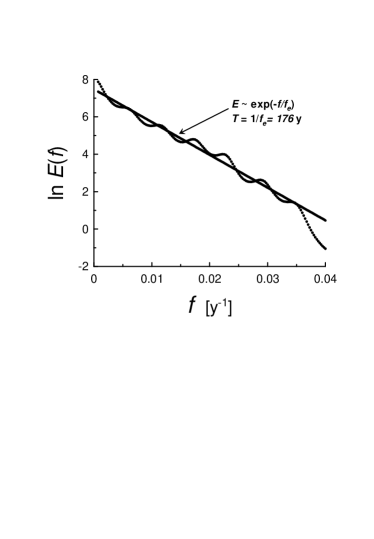
Figure 6: Spectrum of the sunspots number fluctuations in the semi-logarithmic scales for the reconstructed data for the last 11000 years (the data have been taken from Ref. ssn-recon ). The straight line is drawn to indicate the exponential law Eq. (1).

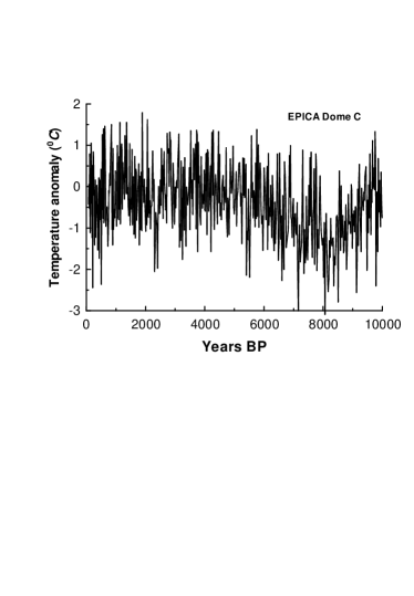
Figure 7: A reconstruction of Antarctic temperature for the past 10,000 years (EPICA Dome C Ice Core EPICA ).

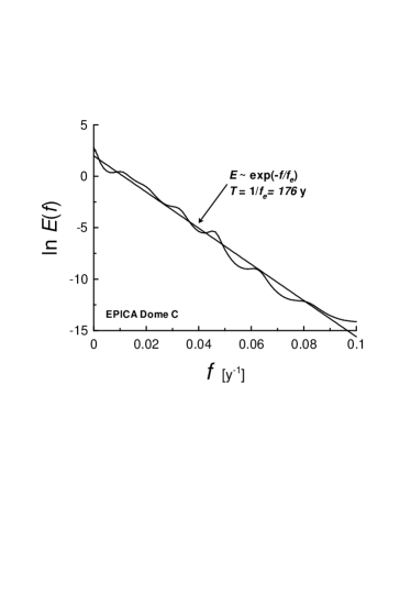
Figure 8: Spectrum of the data, shown in Fig. 7, in semi-logarithmic scales. The straight line indicates the exponential decay Eq. (1).

IV The problem of glaciation cycles

The angle between Earth’s rotational axis and the normal to the plane of its orbit (known as obliquity) varies periodically between 22.1 degrees and 24.5 degrees on about 41,000-year cycle. Such multi-millennium timescale changes in orientation change the amount of solar radiation reaching the Earth in different latitudes. In high latitudes the annual mean insolation (incident solar radiation) decreases with obliquity, while it increases in lower latitudes. Obliquity forcing effect is maximum at the poles and comparatively small in the tropics. Milanković theory suggests that lower obliquity, leading to reduction in summer insolation and in the mean insolation in high latitudes, favors gradual accumulation of ice and snow leading to formation of an ice sheet sal . The obliquity forcing on Earth climate is considered as the primary driving force for the cycles of glaciation (see for a recent review rh ). Observations show that glacial changes from -1.5 to -2.5 Myr (early Pleistocene) were dominated by 41 kyr cycle hC ,rm ,h1 , whereas the period from 0.8 Myr to present (late Pleistocene) is characterized by approximately 100 kyr glacial cycles hays ,im . While the 41 kyr cycle of early Pleistocene glaciation is readily related to the 41 kyr period of Earth’s obliquity variations the 100 kyr period of the glacial cycles in late Pleistocene still presents a serious problem. Influence of the obliquity variations on global climate started amplifying around 2.5 Myr, and became nonlinear at the late Pleistocene. Long term decrease in atmospheric $CO_{2}$, which could result in a change in the internal response of the global carbon cycle to the obliquity forcing, has been mentioned as one of the principal reasons for this phenomenon (see, for instance, berg1 -clar ). Therefore, investigation of the historic variability in atmospheric $CO_{2}$ can be crucial for understanding the global climate changes at millennial timescales.

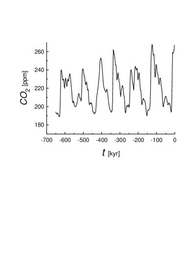
Figure 9: A reconstruction of atmospheric $CO_{2}$ based on deep-sea proxies, for the past 650kyr.

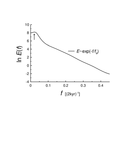
Figure 10: Spectrum of atmospheric $CO_{2}$ fluctuations for the data shown in Fig. 9

Figure 9 shows a reconstruction of atmospheric $CO_{2}$ based on deep-sea proxies, for the past 650kyr (the data taken from berg-data ). Resolution of the data set is 2kyr. Fluctuations with time-scales less than 2kyr could be rather large (statistically up to 308ppm berg-data ), but they are smoothed by the resolution. Figure 10 shows a power spectrum of the data set calculated using the maximum entropy method. The spectrum exhibits a peak indicating a periodic component (the arrow in the Fig. 10 indicates a 100kyr period) and a broad-band part with exponential decay. A semi-logarithmic plot was used in Fig. 10 in order to show the exponential decay more clearly (at this plot the exponential decay corresponds to a straight line). From Fig. 10 we obtain $T_{fun}\simeq 95\pm 8$ kyr (the peak is quite broad due to small data set) and $T_{e}\simeq 41\pm 1$ kyr (the estimated errors are statistical ones). Thus, the obliquity period of 41 kyr is still a dominating factor in the chaotic $CO_{2}$ fluctuations, although it is hidden for linear interpretation of the power spectrum. In the nonlinear interpretation the additional period $T_{fun}\simeq 100$ kyr might correspond to the fundamental frequency of the underlying nonlinear dynamical system and it determines the apparent 100 kyr ’periodicity’ of the glaciation cycles for the last 650 kyr (cf Refs. sal ,ru ,hug1 and references therein). And again, as in the above considered case of the global temperature fluctuations, one cannot rule out a possibility that the broad peak, in a vicinity of frequency corresponding to the 100 kyr period, is a quasi-linear response of the atmospheric $CO_{2}$ to the weak periodic modulation by the 100 kyr cyclicity in the orbital eccentricity variations sha . I.e. again, strong enough periodic forcing results in the non-linear (chaotic) response whereas a weak periodic component of the forcing can result in a quasi-linear (periodic) response.

The author is grateful to W.H. Berger, to V. Masson-Delmotteto, to A. Moberg, to J.J. Niemela and I.G. Usoskin for sharing their data and discussions.

References

- (1) J.P. Gollub, and S. V. Benson, Phys. Rev. Lett., 41, 948 (1978).
- (2) G. Ahlers, P. C. Hohenberg, and M. Lücke, Phys. Rev. A, 32, 3493 (1985).
- (3) M. Franz, and M. Zhang, Phys. Rev. E, 52, 3558 (1995).
- (4) Y. Braiman and I. Goldhirsch, Phys. Rev. Lett., 66, 2545-2548 (1991).
- (5) R. Chacón and J.D. Bejarano, Phys. Rev. Lett., 71, 3103 (1993).
- (6) T. Tamura, N. Inaba, and J. Miyamichi, Phys. Rev. Lett., 83, 3824 (1999).
- (7) P. Huybers, Science, 313, 508 (2006).
- (8) B. Saltzman, Dynamical paleoclimatology : generalized theory of global climate change. (Academic Press, San Diego, 2001).
- (9) The data are available at http://www.ncdc.noaa.gov/ paleo/metadata/noaarecon-6267.html
- (10) A. Moberg, D. M. Sonechkin, K. Holmgren, N. M. Datsenko and W. Karlén, Nature, 433, 613 (2005).
- (11) N. Ohtomo, K. Tokiwano, Y. Tanaka et. al., J. Phys. Soc. Jpn. 64 1104 (1995).
- (12) J. D. Farmer, Physica D, 4, 366 (1982).
- (13) D.E. Sigeti, Phys. Rev. E, 52, 2443 (1995).
- (14) L. A. Safonov, E. Tomer, V. V. Strygin, Y. Ashkenazy, and S. Havlin, Europhys. Lett., 57, 151 (2002).
- (15) U. Frisch and R. Morf, Phys. Rev., 23, 2673 (1981).
- (16) K. Mursula, I. G. Usoskin, and G. A. Kovaltsov, Solar Phys., 198, 51 (2001).
- (17) C.H Gibson, Proc. Roy. Soc. Lond., 434, 149 (1991).
- (18) J. Cho, A. Lazarian, and E.T. Vishniac, Astrophys. J. 564, 291 (2002) (see also arXiv:astro-ph/0205286).
- (19) C.H. Gibson, R.N. Keeler, V.G. Bondur, et al., Proc. of SPIE, 6680, 6680-33 (2007).
- (20) I. G. Usoskin and G. A. Kovaltsov, J. Geophys. Res., 111, D21206, (2006).
- (21) N.J. Shaviv, J. Geophys. Res. 110, A08105 (2005).
- (22) J. Kirkby, Surveys in Geophysics, 28, 333 (2007).
- (23) A. Bershadskii, Physica A, 388, 3213 (2009).
- (24) The data are available at http://www1.ncdc.noaa.gov/ pub/data/paleo/climate_forcing/solar_variability/usoskin-cosmic-ray.txt (see also I.G. Usoskin, K. Mursula, S.K. Solanki, M. Schuessler, and G.A. Kovaltsov, J. Geophys. Res., J. Geophys. Res., 107(A11), 1374 (2002)).
- (25) A. Bershadskii, Phys. Rev. Lett., 90, 041101 (2003).
- (26) A. Bershadskii, Europhys. Lett., 85, 49002 (2009).
- (27) The data are available at http://www1.ncdc.noaa.gov/pub/data/paleo/climate forcing/solar variability/usoskin-cosmicray. txt (see also I.G. Usoskin, K. Mursula, S.K. Solanki, M. Schuessler, and G.A. Kovaltsov, J. Geophys. Res., J. Geophys. Res., 107(A11), 1374 (2002)).
- (28) K.R. Sreenivasan and R.A. Antonia, Annu. Rev. Fluid Mech., 29, 435 (1997).
- (29) The data are available at ftp://ftp.ncdc.noaa.gov/pub/data/paleo/icecore/ antarctica/epica_domec/edc3deuttemp2007.txt (see also J. V. Masson-Delmotte et al., Science, 317, 793 (2007)).
- (30) M. Raymo and P. Huybers P., Nature 451, 284 (2008).
- (31) M. Raymo, and K. Nisancioglu, Paleoceanography, 18, 1011 (2003)
- (32) P. Huybers, Quaternary Sci. Rev., 26, 37 (2007).
- (33) J. Hays, J. Imbrie, and N. Shackleton, Science, 194, 1121 (1976).
- (34) J. Imbrie, E.A. Boyle, S.C. Clemens, et al., Paleoceanography, 7, 701 (1992).
- (35) A. Berger, X. Li, and M.F. Loutre, Quaternary Science Reviews, 18, 1 (1999).
- (36) W.F. Ruddiman, Quaternary Science Reviews, 22, 1597 (2003).
- (37) P. Clark, D. Archer, D. Pollard, J. Blum, J., et al., Quaternary Sci. Rev., 25, 3150 (2006).
- (38) W.H. Berger, Database for reconstruction of atmospheric CO2 in the Milankovitch Chron, IGBP PAGES/World Data Center-A for Paleoclimatology Data Contribution Series # 96-031. NOAA/NGDC Paleoclimatology Program, Boulder CO, USA (see also W.H.Berger, T.Bickert, M.K.Yasuda, G.Wefer, Geologische Rundschau 85, 466 (1996)).
- (39) P. Huybers, Clim. Past Discuss., 5, 237 (2009).
- (40) N.J. Shackleton, Science, 289, 1897 (2000).