Genetic algorithms and supernovae type Ia analysis

Abstract

We introduce genetic algorithms as a means to analyze supernovae type Ia data and extract model-independent constraints on the evolution of the Dark Energy equation of state $w(z)\equiv\frac{P_{DE}}{\rho_{DE}}$. Specifically, we will give a brief introduction to the genetic algorithms along with some simple examples to illustrate their advantages and finally we will apply them to the supernovae type Ia data. We find that genetic algorithms can lead to results in line with already established parametric and non-parametric reconstruction methods and could be used as a complementary way of treating SNIa data. As a non-parametric method, genetic algorithms provide a model-independent way to analyze data and can minimize bias due to premature choice of a dark energy model.

I Introduction

The accelerated expansion of the universe has been confirmed during the last decade by several observational probes Riess:2004nr ; Spergel:2006hy ; Readhead:2004gy ; Goldstein:2002gf ; Rebolo:2004vp ; Tegmark:2003ud ; Hawkins:2002sg . The origin of this acceleration may be attributed to either dark energy with negative pressure, or to a modification of General Relativity that makes gravity repulsive at recent times on cosmological scales. One way to distinguish between these two possibilities and identify in detail the gravitational properties of dark energy or modified gravity is to have a detailed mapping of the expansion rate $H(z)$ as a function of the redshift $z$. This is equivalent to identifying the dark energy equation of state $w(z)\equiv\frac{P}{\rho}$ which can be written as

$$w(z)\,=\,-1\,+\frac{1}{3}(1+z)\frac{d\ln(\delta H(z)^{2})}{d\ln z}\,,{}$$ (1)

where $\delta H(z)^{2}=H(z)^{2}/H_{0}^{2}-\Omega_{\rm 0m}(1+z)^{3}$ accounts for all terms in the Friedmann equation not related to matter. The cosmological constant ($w(z)=-1$) corresponds to a constant dark energy density, while in general it can be time dependent.

It has been shown Vikman:2004dc that a $w(z)$ observed to cross the line $w(z)=-1$ (phantom divide line) is very hard to accommodate in a consistent theory in the context of General Relativity. On the other hand, such a crossing can be easily accommodated in the context of extensions of General Relativity Boisseau:2000pr . Therefore, the crossing of the phantom divide line $w=-1$ could be interpreted as a hint in the direction of modified gravity, see for example Boisseau:2000pr , Bamba:2008hq ,Nesseris:2006er . Such a hint would clearly need to be verified by observations of linear density perturbation evolution through e.g. weak lensing Refregier:2006vt or the redshift distortion factor Hamilton:1997zq .

Early SNIa data put together with more recent such data through the Gold dataset Riess:2004nr ; Riess:2006fw have been used to reconstruct $w(z)$, and have demonstrated a mild preference for a $w(z)$ that crossed the phantom divide line Nesseris:2005ur ; Nesseris:2006er . A cosmological constant remained consistent but only at the $2\sigma$ level. However, the Gold dataset has been shown to suffer from systematics due to the inhomogeneous origin of the data Nesseris:2006ey . More recent SNIa data (SNLSAstier:2005qq , ESSENCEWoodVasey:2007jb , HSTRiess:2006fw ) re-compiled in Davis:2007na have demonstrated a higher level of consistency with $\Lambda$CDM and showed no trend for a redshift dependent equation of state.

However, despite the recent progress the true nature of Dark Energy still remains a mystery with many possible candidates being investigated, see for example Perivolaropoulos:2006ce . The simplest possible candidate assumes the existence of a positive cosmological constant which is small enough to have started dominating the universe at recent times. This model provides an excellent fit to the cosmological observational data Komatsu:2008hk and has the additional bonus of simplicity and a single free parameter. Despite its simplicity and good fit to the data, this model fails to explain why the cosmological constant is so unnaturally small as to come to dominate the universe at recent cosmological times, a problem known as the coincidence problem and there are specific cosmological observations which differ from its predictions Perivolaropoulos:2008ud ,Perivolaropoulos:2008yc .

A further complication in the investigation of the behavior of dark energy occurs due to the bias introduced by the parameterizations used. At the moment, there is a multitude of available phenomenological ansätze for the dark energy equation of state parameter $w$, each with its own merits and limitations (see Sahni:2006pa and references therein). The interpretation of the SNIa data has been shown to depend greatly on the type of parametrization used to perform a data fit Sahni:2006pa . Choosing a priori a model for dark energy can thus adversely affect the validity of the fitting method and lead to compromised or misleading results. The need to counteract this problem paved the way for the consideration of a complementary set of non-parametric reconstruction techniques Daly:2003iy ; Wang:2003gz ; Saini:2003pa . These try to minimize the ambiguity due to a possibly biased assumption for $w$ by fitting the original datasets without using any parameters related to some specific model. The result of these methods can then be interpreted in the context of a DE model of choice. Non-parametric reconstructions can thus corroborate parametric methods and provide more credibility. However, they too suffer from a different set of problems, mainly the need to resort to differentiation of noisy data, which can itself introduce great errors.

In this paper, we consider a method for non-parametric reconstruction of the dark energy equation of state parameter $w$, based on the notions of genetic algorithms and grammatical evolution. We show how the machinery of genetic algorithms can be used to analyze SNIa data and provide examples of its application to determine dark energy parameters for specific models. Our results are consistent with already known findings of both parametric and non-parametric treatments. In particular, we obtain parameters which agree within $1\sigma$ with $\Lambda CDM$, but show a slight trend towards a varying parameter $w(z)$. As a non-parametric method, genetic algorithms provide a model-independent way to analyze data and can minimize bias due to premature choice of a dark energy model.

A rather formal definition of the Genetic Algorithms (GA) Goldberg is that of a computer simulation in which a solution to some predefined problem is searched for in a stochastic way by evolving an ensemble (population) of candidate solutions (usually called chromosomes) towards an optimal state, where some of the chromosomes have reached sufficiently close to the true solution. This approach to problem solving resembles the evolutionary pattern encountered in nature, where an optimal or dominant organism emerges through a series of apparently random mutations and combinations between different individuals. The concept of optimality of a chromosome is usually encoded in the genetic algorithm language in a fitness function, corresponding to the phenotype of an individual. Candidate solutions with a higher fitness function are considered to be better than the rest of the population, in the sense that they are closer to the true solution. Genetic operators such as mutation and combination (crossover) are then implemented to produce offspring from a given population with better properties. Chromosomes with a good fitness are usually more likely to crossover and produce descendants and the combination often takes place between the best candidate solutions of a generation. It is thus more likely for descendants to bear a combination of already favorable genes, leading to an improvement in fitness. The genetic algorithm method is in a way similar to search algorithms, such as hill climbing, $A^{*}$alphastar or simulated annealingannealing .

GAs are more useful and efficient than usual techniques when

• The parameter space is very large, too complex or not enough understood.

• Domain knowledge is scarce or expert knowledge is difficult to encode to narrow the search space.

• Traditional search methods give poor results or completely fail.

so naturally they have been used with success in many fields where one of the above situations is encountered, like the computational science, engineering and economics. Recently, they have also been applied to study high energy physics Becks:1994mm ,Allanach:2004my , Rojo:2004iq gravitational wave detection Crowder:2006wh and gravitational lensing Brewer:2005ww . Since the nature of Dark Energy still remains a mystery, this makes it for us an ideal candidate to use the GAs as a means to analyze the SNIa data and extract model independent constraints on the evolution of the Dark Energy equation of state $w(z)$. In Section 2 we will briefly describe the standard way of analyzing SNIa data while a more thorough treatment of GAs and grammatical evolution (GE) is deferred to Section 3. Section 4 contains the general methodology of the GA paradigm and its application to Supernovae data.

II The Standard SNIa data analysis

We use the SNIa dataset of Kowalski et. al. Kowalski:2008ez consisting of 414 SNIa, reduced to 307 points after various selection cuts were applied in order to create a homogeneous and high-signal-to-noise dataset. These observations provide the apparent magnitude $m(z)$ of the supernovae at peak brightness after implementing the correction for galactic extinction, the K-correction and the light curve width-luminosity correction. The resulting apparent magnitude $m(z)$ is related to the luminosity distance $D_{L}(z)$ through

$$m_{th}(z)={\bar{M}}(M,H_{0})+5log_{10}(D_{L}(z))\,,$$ (2)

where in a flat cosmological model

$$D_{L}(z)=(1+z)\int_{0}^{z}dz^{\prime}\frac{H_{0}}{H(z^{\prime};\Omega_{\rm 0m},w_{0},w_{1})}\,,$$ (3)

is the Hubble free luminosity distance ($H_{0}d_{L}$), and ${\bar{M}}$ is the magnitude zero point offset and depends on the absolute magnitude $M$ and on the present Hubble parameter $H_{0}$ as

$${\bar{M}} = M+5log_{10}\left(\frac{H_{0}^{-1}}{Mpc}\right)+25=$$ (4)

$$= M-5log_{10}h+42.38.$$

The parameter $M$ is the absolute magnitude which is assumed to be constant after the above mentioned corrections have been implemented in $m(z)$.

The SNIa datapoints are given, after the corrections have been implemented, in terms of the distance modulus

$$\mu_{obs}(z_{i})\equiv m_{obs}(z_{i})-M.$$ (5)

The theoretical model parameters are determined by minimizing the quantity

$$\chi^{2}_{SNIa}(\Omega_{\rm 0m},w_{0},w_{1})=\sum_{i=1}^{N}\frac{(\mu_{obs}(z_{i})-\mu_{th}(z_{i}))^{2}}{\sigma_{\mu\;i}^{2}}\,,$$ (6)

where $N=307$ and $\sigma_{\mu\;i}^{2}$ are the errors due to flux uncertainties, intrinsic dispersion of SNIa absolute magnitude and peculiar velocity dispersion. These errors are assumed to be Gaussian and uncorrelated. The theoretical distance modulus is defined as

$$\mu_{th}(z_{i})\equiv m_{th}(z_{i})-M=5log_{10}(D_{L}(z))+\mu_{0}\,,$$ (7)

where

$$\mu_{0}=42.38-5log_{10}h\,,$$ (8)

and $\mu_{obs}$ is given by (5). The steps we followed for the usual minimization of (6) in terms of its parameters are described in detail in Refs. Nesseris:2004wj ; Nesseris:2005ur ; Nesseris:2006er .

This approach assumes that there is some theoretical model available, given in the form of $H(z;p_{i})$ and in terms of some parameters $p_{i}$ like the $\Omega_{\rm 0m}$ or the $w_{0}$ and $w_{1}$ of the CPL ansätz, which is to be compared against the data. As a result of the analysis, the best-fit parameter values and the corresponding $1\sigma$ error bars are obtained. The problem with this method is that the obtained values of the parameters are model-dependent and in general models with more parameters tend to give better fits to the data. This is where the GA approach starts to depart from the ordinary parametric method. Our goal is to minimize a function like (6), not using a candidate model function for the distance modulus and varying parameters, but through a stochastic process based on a GA evolution. This way, no prior knowledge of a dark energy models is needed to obtain a solution. The resulting “theoretical” expression for $\mu_{th}(z)$ is completely parameter-free. This is the main reason for the use of GA in this paper. We now proceed to give a more thorough treatment of GAs and the results of their application in the next sections.

III Genetic algorithms

III.1 Overview

GAs were introduced as a computational analogy of adaptive systems. They are modelled loosely on the principles of the evolution via natural selection, employing a population of individuals that undergo selection in the presence of variation-inducing operators such as mutation and crossover. The encoding of the chromosomes is called the genome or genotype and is composed, in loose correspondence to actual DNA genomes, by a series of representative “genes”. Depending on the problem, the genome can be a series (vector) of binary numbers, decimal integers, machine precision integers or reals or more complex data structures. As mentioned in the introduction, a fitness function is used to evaluate individual chromosomes and reproductive success usually varies with fitness. The fitness function is a map between the gene sequence of the chromosomes (genotype) and a number of attributes (phenotype), directly related to the properties of a wanted solution. Often the fitness function is used to determine a “distance” of a candidate solution from the true one. Various distance measures can be used for this purpose (Euclidean distance, Manhattan, Mahalanobis etc.).

The algorithm begins with an initial population of candidate solutions, which is usually randomly generated. Although GA’s are relatively insensitive to initial conditions, i.e. the population we start from is not very significant, using some prescription for producing this seed generation can affect the speed of convergence. In each successive step, the fitness functions for the chromosomes of the population are evaluated and a number of genetic operators (mutation and crossover) are applied to produce the next generation. This process continues until some termination criteria is reached, e.g. obtain a solution with fitness greater than some predefined threshold or reach a maximum number of generations. The later is imposed as a condition to ensure that the algorithm terminates even if we cannot get the desired level of fitness.

The various steps of the algorithm can be summarized as follows:

1. Randomly generate an initial population $M(0)$

2. Compute and save the fitness for each individual m in the current population $M(t)$.

3. Define selection probabilities $p(m)$ for each individual $m$ in $M(t)$ so that $p(m)$ is proportional to the fitness.

4. Generate $M(t+1)$ by probabilistically selecting individuals from $M(t)$ to produce offspring via genetic operators.

5. Repeat step 2 until satisfying solution is obtained, or maximum number of generations reached.

The paradigm of GAs descibed above is usually the one applied to solving most of the problems presented to GAs. Though it might not find the best solution, more often than not, it would come up with a partially optimal solution.

III.2 Grammatical evolution

The method of grammatical evolution (GE) was first introduced as an alternative approach to genetic programmingONeil ; ONeil2 . Genetic programming is a variation of GAs, which uses programming trees as chromosomes instead of vectors of binary numbers or strings. These chromosomes can be used to express formal expressions, mathematical functions or even entire programs written in some specific programming language. GA operators such as mutation or crossover can then be interpreted as operations which alter or exchange subtrees of a chromosome tree, or splice together two distinct trees.

Grammatical evolution can also be used to produce arbitrary programs in any programming language but without the need for tree structures, which usually require complicated and cumbersome methods to implement genetic operators. Instead, one can use GE to produce an expression or program using an ordinary binary vector chromosome and a generative grammar, which maps the chromosome to an expression using a set of grammatic rules. These rules are usually expressed in a Backus-Naur form (BNF), which can be used to recursively convert a binary vector into a string of terminal symbols, which corresponds to the output. In this way, GE introduces an additional layer of abstraction between the genome (vector of binaries) and the phenotype (fitness). Usually, the transition between the two is accomplished in one step, by evaluating the fitness function of a chromosome. In the case of grammatical evolution, there is the additional step of converting the initial chromosome into an expression using the available grammar. The expression is then evaluated to find the fitness of the chromosome. GA operators can be easily implemented in this scheme on the level of vector chromosomes, since the formal expressions are evaluated in the next step and are not necessary to perform the mutation and crossover. The added abstraction layer also is more similar to what occurs in nature, where a transcription process is used to map DNA base sequences (genotype) into proteins (phenotype). GE has already been applied to problem such as symbolic regressionONeil2 , minimizationTsoulos , robot controlCollins and financeBrabazon .

III.3 Initialization

The first stage of the algorithm involves the creation of an initial population. The chromosomes are generated in a random way and in large enough quantities. The size of the population is very important to successfully mimic a natural selection process, as diversity is crucial to produce a variety of genes and phenotypes. It is thus advisable to use as large a population sample as possible in a simulation, while keeping computational complexity under control. Usually the chromosome count remains fixed throughout the evolutionary phase. Typically this involves a few hundreds, up to several thousands of individuals, although these numbers vary with the type of the problem and the resources available. Similarly, the size of each chromosome (number of genes) is going to affect the speed of the algorithm and the quality of the final solution. Large genomes lead to richer phenotypes and better chances to increase the fitness through mutation and crossover, at the expense of computational efficiency.

III.4 Selection

The purpose of this phase is to select the chromosomes in the population which are going to breed to give a new generation. This is the step where the equivalent of natural selection takes place. Chromosomes are chosen for crossover based on their fitness. Solutions with a better fitness function are the dominant members of the population, hence they are more likely to be selected to produce offspring.

Selection is performed in a stochastic way to avoid premature convergence on suboptimal solutions. The algorithm assigns some selection probability to each chromosome according to its fitness function. The totality of the population or some part of it can be used to draw a number of candidates for crossover. The most popular and heavily used methods for selection are:

• Roulette wheel selection.

• Tournament selection.

In the case of roulette wheel selection, a probability for crossover of a chromosome is considered to be proportional to its fitness. This is a widely used method, but suffers from a number of drawbacks. Since chromosomes with higher fitness are more likely to be selected for crossover, once a suboptimal solution occurs, it may dominate the mating pool. At the same time, less favored chromosomes tend to be completely neglected as candidates for breeding. This leads to premature convergence to suboptimal solutions and stagnation of the evolutionary computation. Roulette wheel selection is also not so easy to implement.

On the other hand, tournament selection chooses the candidates for crossover by taking smaller groups of randomly selected individuals and picking the dominant member of each group. This is an easy algorithm to implement and also more in line with what we usually encounter in nature. Suboptimal chromosomes are thus more likely to be picked than in the roulette wheel case and premature convergence can be avoided more effectively. Tournament selection is going to be used in our treatment of SNIa data.

III.5 Reproduction

After selecting the candidates for breeding, the next step is to combine the corresponding genomes to produce the members of the next generation. This is achieved by the application of genetic operators, mutation and crossover.

For each pair of parent chromosomes picked from the population, two children chromosomes are produced by exchanging the genomes of the two parents. The easiest and more popular method is one-point crossover, where a particular point is chosen on the genome sequence and the genes from that point on completely exchanged between the chromosomes. The descendants are then subjected to mutation with some predefined probability (mutation rate). This process of selection/crossover/mutation is then repeated until enough individuals are produced to form a new generation. More often the entire population of the previous generation is replaced by members produced during the reproduction stage. In some cases, elitism is applied to ensure that some of the already found solution with the best fitnesses are passed on to the next generation. Although the two parent scheme is more biology inspired, recent researches suggested more than two parents may lead to better quality chromosomes.

By crossover and mutation, a new generation with different members from the progenitor is created. New chromosomes tend to inherent the best qualities of the previous generation, since members with higher fitness are more likely to be selected for reproduction. In general, the new chromosomes will have better fitnesses on the average and a better maximum fitness within the population.

III.6 Termination

The GA evolution continues until a termination condition has been reached. Some of the most common conditions for termination include:

• An optimal solution is found based on some best fitness threshold.

• The maximum number of generations is reached.

• Allocated budget (CPU time/money) reached.

• Further execution doesn’t significantly improve the best fitness in the population.

• Combinations of the above.

IV Results

IV.1 General Methodology

We first outline the course of action we follow to apply the GA paradigm in the case of SNIa data. For the application of GA and GE on the dataset, we use a modified version of the GDFTsoulos tool  , which uses GE as a method to fit datasets of arbitrary size and dimensionality. This program uses the tournament selection method for crossover. GDF requires a set of input data (train set), an (optional) test sample and a grammar to be used for the generation of functional expressions. The output is an expression for the function which best fits the train set data.

In our case, the train set is the SNIa dataset, containing 307 pairs of the distance modulus $\mu(z)$ and the redshift $z$ as described in Section 2. We also modify GDF to read an additional file containing the errors of the corresponding data points, which are used to evaluate the fitness function. No test dataset is needed for our purposes.

The grammar used may involve standard numerical operations ($+,-,*,/$, etc.), as well as typical functions such as $sin,cos,log,exp$ etc. and more complex production rules to turn non-terminal expressions into terminal symbols. The choice of the grammar vocabulary is apparently crucial for the behavior of the algorithm, the speed of convergence and the quality of the final fit. Our goal is to obtain a smooth fit for the distance modulus curve in the range of $0\leq z\leq 1.75$, which will not lead to problematic behavior upon differentiation and can produce a high goodness of fit. The use of the $abs$ function is initially excluded, since as it turns out is prone to lead to discontinuities and unphysical behavior of the resulting dark energy profile. Periodic functions may also lead to high frequency oscillatory behavior in the candidate solutions, as the fitting function attempts to interpolate between densely spaced fluctuating datapoints. Solutions of this sort generally seem to yield a better goodness of fit compared to grammars not employing periodic functions. Such oscillatory behavior is hard to distinguish within the accuracy available and there is little theoretical justification to take it into account. We also find that this family of grammars in the end yields higher errors for the final model parameters, once a particular dark energy model is tested using the periodic solutions. We thus choose to exclude functions such as $sin$ and $cos$ for our final treatment of SNIa data.

It is important to note that the method we discuss is highly non-parametric. By this we mean that no parameters are used in the process of fitting the initial dataset to obtain a candidate solution. The GA does not apply some kind of minimization using a seed parametric function. Instead, the maximization of the best population fitness, which is equivalent to a $\chi^{2}$ minimization procedure, is accomplished in a purely stochastic way. The resulting solution is given as an ordinary formal mathematical expression of a function of $z$, in which no parameters appear. This should be contrasted to other non-parametric dark energy reconstruction methods, where some sort of parameter minimization takes place from the very beginning, even if these parameters are not directly related to some specific dark energy model and only later do they get mapped to some corresponding set of model-dependent quantitiesDaly:2003iy . This is an advantage of the GA approach, as it minimizes the amount of initial model-dependent bias. Strictly speaking, the only parameter which can be tuned beforehand is the vocabulary of the grammar used. Grammatical evolution ameliorates this potential source of bias, since it possesses a far greater expressive power than ordinary fit methods used, such as bin-wise polynomial fits. The apparent drawback of the GA is that it is in the end overly non-parametric, to the point where no established tools used in usual minimization techniques can be employed to estimate and propagate errors. We will discuss later how this problem can be bypassed.

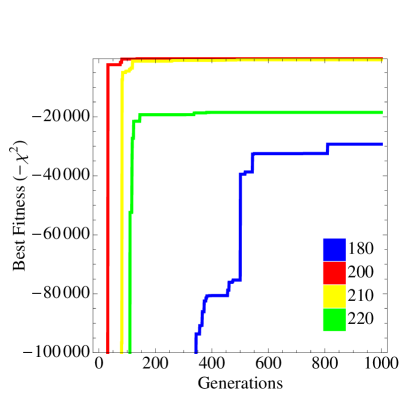
Figure 1: Convergence of the genetic algorithm as a function of the number of generations. Curves are presented for different values of the total number of chromosomes in the population. The case with 190 chromosomes converges very slowly for the original SNIa dataset and is omitted.

The fitness function for the GA is chosen to be equal to $-\chi^{2}_{SNIa}$, where

$$\chi^{2}_{SNIa}=\sum_{i=1}^{N}\frac{(\bar{\mu}_{obs}(z_{i})-\bar{\mu}_{GA}(z_{i}))^{2}}{\sigma_{\mu\;i}^{2}}\,,$$ (9)

and $\bar{\mu}(z)=\mu(z)-\mu_{0}$. Notice the differences compared with (6). The $\chi^{2}_{SNIa}$ doesn’t depend on parameters and $\bar{\mu}_{GA}(z)$ is the reduced distance modulus obtained for each chromosome of the population through GE. We opt to fit for $\bar{\mu}(z)$ instead of $\mu(z)$, since the non-parametric approach we use prevents us from marginalizing over $\mu_{0}$.

Another advantage is the fact that the GA does not require an assumption of flatness as it can be seen from eq. (6), since it was used in order to find the reduced distance modulus $\mu(z)$. Flatness (or non-flatness) comes into play when one tries to find the luminosity distance $D_{L}(z)$ and the underlying dark energy model given $\mu_{GA}(z)$. So, in this aspect the GA is independent of the assumption of flatness as well.

The GA evaluates (9) in each evolutionary step for every chromosome of the population. The one with the best fitness will consequently have the smallest $\chi^{2}_{SNIa}$ and will be the best candidate solution in its generation. Of all the steps in the execution of the algorithm, the evaluation of the fitness is the most expensive. GDF is appropriately modified to use (9) as the basis of its fitness calculation.

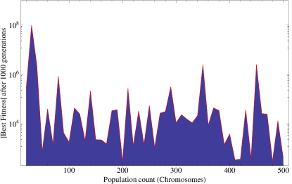
Figure 2: $|Bestfitness|$ (lower is better) after $1000$ generations as a function of the chromosome count in the population.

Additionally, GDF requires a number of parameters which determine the execution of the GA. These include the selection (percentage of the population that goes unchanged into the next generation) and mutation rates, the genome length of chromosomes in the population, and the total chromosome count in one generation. A maximum number of generations is also specified. We keep the default values for the selection rate ($10\%$) and mutation rate ($5\%$).

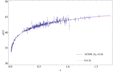
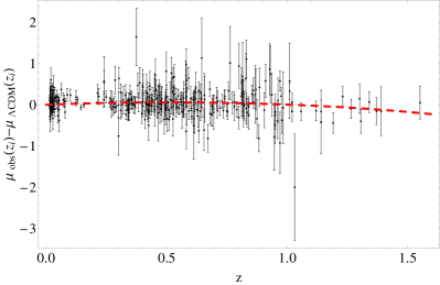
Figure 3: Left: The SNIa distance modulus against the redshift. The solid line represents the $\Lambda CDM$ curve with $\Omega_{m}=0.26$. The dashed line is a GA best fit function of eq. (10). Right: The data and the GA best-fit of eq. (10) residuals relative to $\Lambda CDM$.

The parameters which can significantly change the speed of the algorithm is the genome length and the population size. Given the use of GE, one should bear in mind that very long chromosomes with many genes are not always fully used in the transcription process to produce a formal expression. As such, we deem a chromosome length of $100$ genes long enough, leading to solutions with a high goodness of fit, without being computationally very expensive. Having fixed the chromosome length, we must choose an appropriate population size. Since the fitness function has to be evaluated for every chromosome in one generation, this is the most important parameter for the speed of execution. The GA is a stochastic algorithm and thus the speed of convergence to an optimal solution cannot be easily determined and is affected by a number of parameters.

To find the most suitable population size, we make a preliminary scan of this parameter space for different number of chromosomes and determine what is the best fitness after $1000$ generations. We determine sweet spots for $200$, $410$, $420$, $440$ and $480$ chromosomes. The first of them is used as the chromosome count for the rest of the treatment, as it gives the fastest execution with good results. All tests use an evolution of $1000$ generations.

After the execution of the GA, we obtain an expression $\bar{\mu}_{GA}(z)$ for the reduced distance modulus as the solution of best fitness and the corresponding $\chi^{2}_{SNIa}$. Using this we can, through differentiation, obtain parameters of interest, such as dark energy equation of state parameters in the context of some model. As already mentioned, this method gives no direct way to estimate the errors for the derived parameters. One cannot expect to get an estimate by just running the algorithm many times and obtaining slightly different parameters. The GA usually tends to converge at the same solution for a given dataset, unless we change significantly the population size or the number of generations. A way to circumvent this problem is to use Monte Carlo simulation to produce synthetic datasets and rerun the algorithm on them. We can thus obtain a statistical sample of parameter values which will allow us to estimate the error. We sketch the procedure we follow:

1. The GA is applied on the original SNIa dataset with the chosen execution parameters and a solution for $\bar{\mu}_{GA}(z)$ is obtained.

2. Choosing a particular dark energy model, we determine its DE parameters from $\bar{\mu}_{GA}(z)$ using differentiations. These parameters will be used as seed values to produce synthetic datasets.

3. A large number of synthetic datasets is produced from the DE model, using the seed values from the previous step. We add gaussian noise to the data points to simulate real observational data. The standard deviation for noise is taken to be equal to that of the corresponding observational point.

4. The GA is rerun for the synthetic datasets.

5. A new set of parameter values is determined from the solutions of the synthetic datasets.

6. Outliers are eliminated using recursive trimming to reduce variance of the statistical sample.

7. The final mean values and standard deviations of the DE parameters are determined.

Using the above steps, we can obtain error estimates for the DE model we wish to examine. Step 6 is essential to reduce the number of outliers in the sample. The GA is stochastic and non-linear, so adding gaussian noise to the input data doesn’t lead to a gaussian distribution of the output. For some of the synthetic datasets the algorithm will fail to converge fast enough, yielding a suboptimal solution, hence the presence of outliers. By recursively trimming the sample, we can significantly improve the accuracy of the result.

IV.2 Applications

We will now give a number of examples where the method is applied and the results interpreted in the context of some dark energy model. We first use the GA to treat the more popular $\Lambda CDM$ model, which is also an easier example to demonstrate the method. In the next section we consider a model with a dark energy equation of state parameter which depends on the redshift and determine the appropriate DE parameters of the model.

IV.2.1 $\Lambda CDM$

For $\Lambda CDM$, the properties of dark energy are fully determined, since $w=-1$ and the only free parameter of the model is the total matter density $\Omega_{m}$. As described above, we first run the algorithm on the SNIa dataset to obtain a seed solution for the reduced distance modulus, and thus the distance modulus $\mu_{GA}(z)$. Applying the GA to the original dataset as it is was found to produce solutions with unphysical behavior for small redshift, where we would expect $H(z)\to H_{0}$. For this reason, a fiducial point was added in the dataset at small $z$ with a very low standard deviation, so that every good candidate solution should take it into account. The total $\chi^{2}$ during the GA runs included this artificial point. However, in our subsequent treatment and final results we reverted to the initial dataset (all $\chi^{2}$ values mentioned later do not include the fiducial point). Using this method, the distance modulus was found to be

$$\mu_{GA}(z)=\log\left(z^{2.17145}\left(-z^{2.82}+z+e^{z}\right)\right)+\mu_{0}\,.$$ (10)

Note that eq. (10) is not unique since each time the GA is ran it may give a different but equally good and model independent approximation to the reduced distance modulus $\mu(z)$. This function is then fitted against the corresponding modulus predicted by $\Lambda CDM$

$$\mu_{\Lambda CDM}\left(z\right)=5\log_{10}D_{L}\left({z;\Omega_{m}}\right)+\mu_{0}\,,$$ (11)

with

$$H\left(z\right)^{2}=H_{0}^{2}\left[\Omega_{m}\left({1+z}\right)^{3}+1-\Omega_{m}\right]\,,$$ (12)

to obtain the seed value of $\Omega_{m}$. We then use the Monte Carlo method to produce $100$ synthetic datasets from (11) adding gaussian noise and rerun the GA on them. The resulting set of $\mu_{GA}(z)$ from the synthetic datasets is used to obtain in the same fashion a statistical sample of $\Omega_{m}$ values. Due to the non-linearity of the GA and GE implementation, the sample is not normally distributed and contains a lot of outliers. This is easy to establish both graphically through histograms, or by comparing the mean and standard deviation of the sample with its corresponding robust estimators, the median and median deviation. The large discrepancy between these quantities is a sign of outliers in the dataset. We eliminate these by recursively removing outlier points. The heuristic we use is to discard in each step data points that are more than 2$\sigma$ away from the mean of the distribution at that stage. The trimming continues until we reach a stationary state, where no other points are removed. From the improved statistical sample we determine the final values of the mean and standard deviation for the dark matter density to be $\Omega_{m}=0.308\pm 0.029$, in good agreement with the WMAP value of $\Omega_{m}=0.258\pm 0.030$ Komatsu:2008hk .

Table 1: Comparison of the mean and standard deviation of the $\Omega_{m}$ statistical sample produced from the synthetic datasets and the corresponding median and median deviation. The initial large discrepancy is greatly reduced by trimming outlier points.

	Mean	Median	$\Delta$ ($\%$)	$\sigma$	$\sigma_{median}$	$\Delta$ ($\%$)
Initial	$0.633$	$0.357$	77.5	$0.584$	$0.074$	692
Trimmed	$0.308$	$0.298$	3.26	$0.029$	$0.016$	83.3

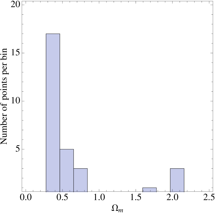
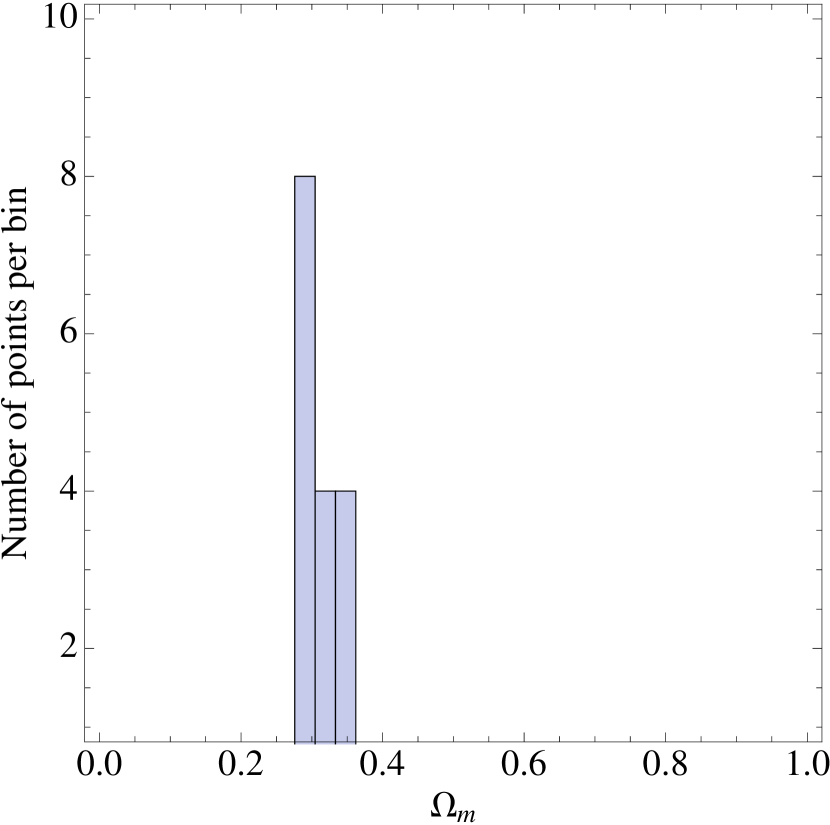
Figure 4: Histograms showing the dispersion of the set of $\Omega_{m}$ values. Upper: Initial set. Lower: After the recursive trimming of outliers.

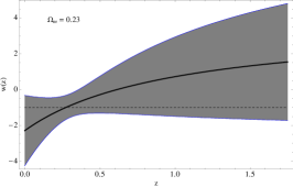
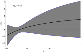
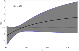
Figure 5: The DE equation of state $w(z)$ for different values of $\Omega_{m}$.

Table 2: Values for mean and median and their corresponding errors for the Chevallier-Polarski-Linder DE ansätz. Large discrepancies between the mean and the median signal the presence of outliers. Overall $\chi^{2}$ can be significantly -and adversely- affected by such points. The trimmed samples generally present a considerably better behavior.

	$\Omega_{m}$	Mean $w_{0}$	Median $w_{0}$	$\Delta w_{0}$ ($\%$)	$\Delta\sigma w_{0}$ ($\%$)	Mean $w_{1}$	Median $w_{1}$	$\Delta w_{1}$ ($\%$)	$\Delta\sigma w_{1}$ ($\%$)	$\chi^{2}$
Initial	0.23	$-1.8\pm 6.9$	$-2.4\pm 1.3$	24.6	$424$	$4\pm 25$	$5.5\pm 5.5$	$23.5$	$345$	352.2
Trimmed	0.23	$-2.3\pm 2.0$	$-2.4\pm 1.1$	$4.7$	$73$	$6.0\pm 7.9$	$5.6\pm 3.8$	$7.7$	$109$	471.0
Initial	0.26	$-9\pm 69$	$2.4\pm 1.5$	278	$4480$	$30\pm 240$	$5.3\pm 7.5$	$456$	$3140$	3797
Trimmed	0.26	$-1.8\pm 1.6$	$-2.2\pm 1.1$	$18.4$	$37.8$	$3.7\pm 6.5$	$5.2\pm 4.7$	$28.8$	$37.8$	343.4
Initial	0.29	$-50\pm 470$	$-2.4\pm 1.2$	$1960$	$38500$	$200\pm 1700$	$4.6\pm 6.6$	$3810$	$25500$	6667
Trimmed	0.29	$-2.3\pm 1.4$	$-2.5\pm 0.8$	$7.9$	$75.5$	$4.4\pm 5.5$	$5.0\pm 3.9$	$12.1$	$48.8$	420.6

IV.2.2 Chevallier-Polarski-Linder DE ansätz

In this dark energy model, the equation of state parameter is given by the ansätz,Chevallier:2000qy ; Linder:2002dt

$$w\left(z\right)=w_{0}+w_{1}\frac{z}{{1+z}}$$ (13)

with two parameters $w_{0}$ and $w_{1}$ determining the temporal profile of $w(z)$. This model has been extensively used in previous parametric reconstructions of dark energy from SNIa data. The distance modulus of the model is given by equations (2) and (3) using

$$H\left(z\right)^{2} = H_{0}^{2}[\Omega_{m}\left({1+z}\right)^{3}$$

$$+ \left({1-\Omega_{m}}\right)\left({1+z}\right)^{3\left({1+w_{0}+w_{1}}\right)}e^{-3w_{1}\frac{z}{{1+z}}}]\,.$$

Here we use the matter density as an input parameter and attempt to reconstruct the dark energy profile by determining the two DE parameters $w_{0}$ and $w_{1}$. We repeat the process three times using as $\Omega_{m}$ the WMAP value $\pm 1\sigma$. As we see in Table 2, the WMAP value gives the best goodness of fit. The method is roughly the same as for $\Lambda CDM$, only now we have to determine two parameters. After running the GA on the SNIa dataset and getting the seed values for $w_{0}$ and $w_{1}$, we produce $100$ synthetic datasets and reapply the algorithm to get a sample of parameter values. Again, we have to remove outlier points to decrease the dispersion of the data. To do so, we recursively remove data points lying outside the $90\%$ confidence level in every step, until we reach a stationary state. From the improved sample values we get the mean and errors for $w_{0}$ and $w_{1}$.

The profiles we get for the DE equation of state parameter are in accordance with previous parametric reconstructions based on this model. We see in Fig. 5 there is a trend for a redshift-varying $w(z)$, with a crossing of the $w=-1$ line at late times. Still, the errors are large for the method to make any conclusive arguments about these effects. The errors are essentially due to the limited number of MC synthetic datasets used for this treatment. Increasing the number of datasets would lead to better statistics and decrease the errors further, but at a great computational cost, since the GA should then be applied to a much larger collection of data.

V Conclusions

We presented a method for non-parametric reconstruction of the dark energy equation of state parameter based on the genetic algorithms paradigm and grammatical evolution. The method was applied to determine parameters of cosmological models such as the $\Lambda CDM$ and the Chevallier-Polarski-Linder DE ansätz. This approach produces results that are in agreement with previous parametric and non-parametric reconstructions. The main advantage of the GA is the absence of any parametrization in the treatment of the initial data which can reduce any model-dependent bias. In our case the desired function to be found is the reduced distance modulus $\mu(z)$. It should be noted that running the GA several times may give different but equally good model independent approximations to the distance modulus $\mu(z)$, so what we actually need some statistics and a model to interpret the results. The reason for this is that if we want to constrain a parameter like $Omega_{m}$, then already we have made a (minimal) assumption for the underlying theory. A similar approach has been also used in the literature before, see for example Allanach:2004my where the authors use the GA to discriminate between the various SUSY models.

On the other hand, the shortcomings of the method include computational speed issues, since the execution of the GA is usually very expensive regarding the CPU time needed. This in turn limits the amount of precision one can obtain using Monte Carlo methods to estimate errors for the final model parameters. However, this issue can soon be resolved with the advent of faster systems and more efficient GA implementations. Other open issues include the determination of optimal algorithm parameters for the SNIa dataset, as well an extension of the method to analyze a larger variety of dark energy models.

References

- (1) A. G. Riess et al. [Supernova Search Team Collaboration], Astrophys. J. 607, 665 (2004).
- (2) D. N. Spergel et al. [WMAP Collaboration], Astrophys. J. Suppl. 170, 377 (2007) [arXiv:astro-ph/0603449].
- (3) A. C. S. Readhead et al., Astrophys. J. 609, 498 (2004) [arXiv: astro-ph/0402359].
- (4) J. H. Goldstein et al., Astrophys. J. 599, 773 (2003) [arXiv:astro-ph/0212517].
- (5) R. Rebolo et al., MNRAS 353 747R (2004) [arXiv:astro-ph/0402466].
- (6) M. Tegmark et al. [SDSS Collaboration], Phys. Rev. D 69, 103501 (2004) [arXiv:astro-ph/0310723]
- (7) E. Hawkins et al., Mon. Not. Roy. Astron. Soc. 346, 78 (2003) [arXiv:astro-ph/0212375]
- (8) A. Vikman, Phys. Rev. D 71, 023515 (2005) [arXiv:astro-ph/0407107].
- (9) B. Boisseau, G. Esposito-Farese, D. Polarski and A. A. Starobinsky, Phys. Rev. Lett. 85, 2236 (2000) [arXiv:gr-qc/0001066]; L. Perivolaropoulos, JCAP 0510, 001 (2005) [arXiv:astro-ph/0504582]; B. Jain and P. Zhang, arXiv:0709.2375 [astro-ph]; S. Nesseris and L. Perivolaropoulos, Phys. Rev. D 73, 103511 (2006) [arXiv:astro-ph/0602053]; A. F. Heavens, T. D. Kitching and L. Verde, arXiv:astro-ph/0703191; V. Sahni and Y. Shtanov, JCAP 0311, 014 (2003) [arXiv:astro-ph/0202346]; C. Bogdanos and K. Tamvakis, Phys. Lett. B 646 (2007) 39 [arXiv:hep-th/0609100]; C. Bogdanos, A. Dimitriadis and K. Tamvakis, Phys. Rev. D 75 (2007) 087303 [arXiv:hep-th/0611094]; Class. Quant. Grav. 24 (2007) 3701 [arXiv:hep-th/0611181]; C. Bogdanos, S. Nesseris, L. Perivolaropoulos and K. Tamvakis, Phys. Rev. D 76 (2007) 083514 [arXiv:0705.3181 [hep-ph]].
- (10) K. Bamba, C. Q. Geng, S. Nojiri and S. D. Odintsov, arXiv:0810.4296 [hep-th].
- (11) S. Nesseris and L. Perivolaropoulos, JCAP 0701, 018 (2007) [arXiv:astro-ph/0610092].
- (12) J. Benjamin et al., arXiv:astro-ph/0703570; C. Shapiro and S. Dodelson, Phys. Rev. D 76, 083515 (2007) [arXiv:0706.2395 [astro-ph]]; L. Amendola, M. Kunz and D. Sapone, arXiv:0704.2421 [astro-ph]; A. Refregier et al., arXiv:astro-ph/0610062.
- (13) A. J. S. Hamilton, arXiv:astro-ph/9708102; E. V. Linder, arXiv:0709.1113 [astro-ph]; S. Nesseris and L. Perivolaropoulos, arXiv:0710.1092 [astro-ph]; C. Di Porto and L. Amendola, arXiv:0707.2686 [astro-ph]; Y. Wang, arXiv:0710.3885 [astro-ph].
- (14) A. G. Riess et al., Astrophys. J. 659, 98 (2007) [arXiv:astro-ph/0611572].
- (15) S. Nesseris and L. Perivolaropoulos, Phys. Rev. D 72, 123519 (2005) [arXiv:astro-ph/0511040].
- (16) S. Nesseris and L. Perivolaropoulos, JCAP 0702, 025 (2007) [arXiv:astro-ph/0612653].
- (17) P. Astier et al. [The SNLS Collaboration], Astron. Astrophys. 447, 31 (2006) [arXiv:astro-ph/0510447].
- (18) W. M. Wood-Vasey et al. [ESSENCE Collaboration], Astrophys. J. 666, 694 (2007) [arXiv:astro-ph/0701041]; G. Miknaitis et al., arXiv:astro-ph/0701043;
- (19) T. M. Davis et al., Astrophys. J. 666, 716 (2007) [arXiv:astro-ph/0701510].
- (20) L. Perivolaropoulos, AIP Conf. Proc. 848, 698 (2006) [arXiv:astro-ph/0601014].
- (21) E. Komatsu et al. [WMAP Collaboration], Astrophys. J. Suppl. 180, 330 (2009) [arXiv:0803.0547 [astro-ph]].
- (22) L. Perivolaropoulos, arXiv:0811.4684 [astro-ph].
- (23) L. Perivolaropoulos and A. Shafieloo, arXiv:0811.2802 [astro-ph].
- (24) V. Sahni and A. Starobinsky, Int. J. Mod. Phys. D 15, 2105 (2006) [arXiv:astro-ph/0610026].
- (25) R. A. Daly and S. G. Djorgovski, Astrophys. J. 597 (2003) 9 [arXiv:astro-ph/0305197].
- (26) Y. Wang and P. Mukherjee, Astrophys. J. 606 (2004) 654 [arXiv:astro-ph/0312192].
- (27) T. D. Saini, Mon. Not. Roy. Astron. Soc. 344, 129 (2003) [arXiv:astro-ph/0302291].
- (28) D.E. Goldberg, “Genetic Algorithms in Search, Optimization and Machine Learning”, Addison-Wesley, 1989.
- (29) P. E. Hart, N. J. Nilsson, B. Raphael, IEEE Transactions on Systems Science and Cybernetics (1968), SSC4 (2): 100–107.
- (30) N. Metropolis, A.W. Rosenbluth, M.N. Rosenbluth, A.H. Teller, and E. Teller, Journal of Chemical Physics, (1953) 21(6):1087-1092, 1953;S. Kirkpatrick, C.D. Gelatt, M.P. Vecchi, Science. New Series 220 (1983) (4598): 671-680;V. Cerny, Journal of Optimization Theory and Applications, (1985) 45:41-51.
- (31) K. H. Becks, S. Hahn and A. Hemker, Phys. Bl. 50 (1994) 238; G. Organtini, Talk given at Computing in High-energy Physics (CHEP 97), Berlin, Germany, 7-11 Apr 1997; M. Mjahed, Nucl. Instrum. Meth. A 559 (2006) 172.
- (32) B. C. Allanach, D. Grellscheid and F. Quevedo, JHEP 0407, 069 (2004) [arXiv:hep-ph/0406277].
- (33) J. Rojo and J. I. Latorre, JHEP 0401, 055 (2004) [arXiv:hep-ph/0401047]; M. C. Gonzalez-Garcia, M. Maltoni and J. Rojo, JHEP 0610, 075 (2006) [arXiv:hep-ph/0607324]; L. Del Debbio, S. Forte, J. I. Latorre, A. Piccione and J. Rojo [NNPDF Collaboration], JHEP 0703, 039 (2007) [arXiv:hep-ph/0701127].
- (34) J. Crowder, N. J. Cornish and L. Reddinger, Phys. Rev. D 73 (2006) 063011 [arXiv:gr-qc/0601036].
- (35) B. J. Brewer and G. F. Lewis, arXiv:astro-ph/0501202.
- (36) M. O’Neill, C. Ryan, IEEE Trans. Evolutionary Comput. 5 (2001) 349-358.
- (37) M. O’Neill, C. Ryan, “Grammatical Evolution: Evolutionary Automatic Programming in an Arbitrary Language”, Genetic Programming, vol. 4, Kluwer Academic Publishers, 2003.
- (38) J.J Collins, C. Ryan, Proc. of AROB 2000, 5th Internat. Symp. on Artificial Life and Robotics, 2000.
- (39) A. Brabazon, M. O’Neill, in: H.R. Arabnia (Ed.), Proc. Internat. Conf. on Artificial Intelligence, vol. II, CSREA Press, 2003, pp. 492-498.
- (40) I.G. Tsoulos, D. Gavrilis, E. Dermatas, Computer Physics Communications 174 (2006) 555-559.
- (41) M. Kowalski et al., Astrophys. J. 686, 749 (2008) [arXiv:0804.4142 [astro-ph]].
- (42) S. Nesseris and L. Perivolaropoulos, Phys. Rev. D 70, 043531 (2004) [arXiv:astro-ph/0401556].
- (43) M. Chevallier and D. Polarski, Int. J. Mod. Phys. D 10, 213 (2001) [arXiv:gr-qc/0009008].
- (44) E. V. Linder, Phys. Rev. D 68, 083503 (2003) [arXiv:astro-ph/0212301].