Partial clustering prevents global crystallization in a binary 2D colloidal glass former

Abstract

A mixture of two types of super-paramagnetic colloidal particles with long range dipolar interaction is confined by gravity to the flat interface of a hanging water droplet. The particles are observed by video microscopy and the dipolar interaction strength is controlled via an external magnetic field. The system is a model system to study the glass transition in 2D, and it exhibits partial clustering of the small particles cluster_prl . This clustering is strongly dependent on the relative concentration $\xi$ of big and small particles. However, changing the interaction strength $\Gamma$ reveals that the clustering does not depend on the interaction strength. The partial clustering scenario is quantified using Minkowski functionals and partial structure factors. Evidence that partial clustering prevents global crystallization is discussed.

1 Influence of dimensionality on frustration

It is well known that the macroscopic behavior of crystalizing systems sensitively depends on dimensionality, as demonstrated by two examples: In 2D an intermediate phase exists between fluid and crystal, the hexatic phase, where the system has no translational order while the orientational correlation is still long-range hexatic_theo ; hexatic_exp ; hexatic_exp2 . Such a two step melting scenario is not known in 3D. The Ising model for ferromagnetics shows a phase transition for 2D and 3D but not for 1D ising . For amorphous systems, however, it was found in experiments hansroland_glass , simulations harrowell_glass_2d , and theory bayer_2d_mct that the glass transition phenomenology is very similar in 2D and 3D systems, both in dynamics and structure hansroland_glass ; epje_ebert .
A subtle difference, the local density optimization in 2D and 3D, is the following: in 3D the local density optimized structure of four spheres is obviously a tetrahedron. However, it is not possible to completely cover space in 3D with tetrahedra, because the angle between two planes of a tetrahedron is not a submultiple of $360\textdegree$ tetraeder . The density optimized state with long-range order is realized by the hexagonal closed packed structure or other variants of the fcc stacking with packing fraction $\phi=\pi/\sqrt{18}\approx 74\%$. The dynamical arrest in 3D is expected to be enhanced by this geometrical frustration, because the system has to rearrange its local density optimized structure to reach long-range order. The local geometrical frustration scenario is different in 2D. There, the local density optimized structure and densest long-range ordered structure are identical, namely hexagonal. For the glass transition in 2D it is therefore expected that an increase of complexity is necessary to reach dynamical arrest without crystallization: in simulations an isotropic one-component 2D system has been observed undergoing dynamical arrest for an inter-particle potential that exhibits two length scales, a Lennard-Jones-Gauss potential with two minima LJG . Other simulations showed that systems of identical particles in 2D can vitrify if the mentioned local geometric frustration is created artificially via an anisotropic fivefold interaction potential tanaka_glass_crystal . Alternatively, the necessary complexity can be created by polydispersity as found in simulations poly_2d .
A bi-disperse system in general is simple enough to crystallize as e.g. seen from the rich variety of binary crystal structures in an oppositely charged 3D coulomb mixture van_bladeren . In the system at hand, partial clustering prevents the homogenous distribution of particles and the system crystallizes locally into that crystal structure which is closest in relative concentration epje_ebert ; dipolar_crystals ; gen_algorithm . In this way the system effectively lowers its energy with a compromise between minimization of particle transport and minimization of potential energy. However, that means that the resulting structure is not in equilibrium, but in a frustrated glassy state. This competition of local stable crystal structures prevents the relaxation into an energetically equilibrated state, i.e. a large mono-crystal.
It was found that a binary mixture of magnetic dipoles is a good model system of a 2D glass former hansroland_glass as the dynamics and structure shows characteristic glassy behavior: when the interaction strength $\Gamma$ is increased, the system viscosity increases over several orders of magnitude while the global structure remains amorphous.
For all measured interaction strengths the system shows no long-range order as probed with bond order correlation functions epje_ebert . However, on a local scale it reveals non-trivial ordering phenomena: partial clustering and local crystallinity.
Partial clustering cluster_prl ; cluster_pre means that the small particles tend to form loose clusters while the big particles are homogeneously distributed. The heterogeneous concentration of small and big particles leads to a variety of local crystal structures when the system is supercooled making up the globally amorphous structure. This local crystallinity obviously plays a key role for the glass transition in this 2D colloidal system as it dominates the glassy structure epje_ebert . Therefore, the phenomenon of partial clustering is indirectly responsible for the frustration towards the glassy state. In section 4 the details of the clustering scenario are explained. The dependence on the parameters accessible in experiment and the relation to local crystallinity epje_ebert are discussed in section 5.

Firstly, the experimental setup is introduced. After a brief discussion about origin of partial clustering, a morphological analysis using Minkowski measures is presented to characterize and quantify the effect. Finally, the dependence on relevant parameters like the average relative concentration $\xi$ and the interaction strength $\Gamma$ will be discussed using Euler characteristics and the partial static structure factors.

2 Experimental setup

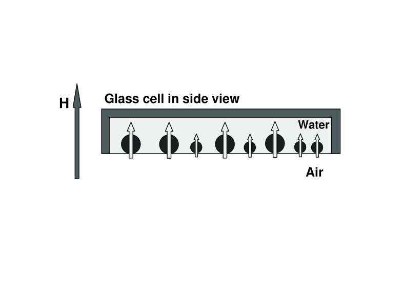
Figure 1: Super-paramagnetic colloidal particles confined at a water/air interface due to gravity. The curvature of the interface is actively controlled to be completely flat; therefore the system is considered to be ideal two dimensional. A magnetic field H perpendicular to the interface induces a magnetic moment m in each bead leading to a repulsive dipolar interaction.

The detailed experimental setup is explained in sci_instr . It consists of a mixture of two different kinds of spherical and super-paramagnetic colloidal particles (species A: diameter $d_{A}=4.5\>\mu m$, susceptibility $\chi_{A}=7.4\cdot 10^{-11}\>Am^{2}/T$, density $\rho_{A}=1.5\>g/cm^{3}$ and species B: $d_{B}=2.8\>\mu m$, $\chi_{B}=6.6\cdot 10^{-12}\>Am^{2}/T$, $\rho_{B}=1.3\>g/cm^{3}$) which are confined by gravity to a water/air interface. This interface is formed by a water drop suspended by surface tension in a top sealed cylindrical hole ($6\>mm$ diameter, $1\>mm$ depth) of a glass plate as sketched in Fig. 1. A magnetic field $\vec{H}$ is applied perpendicular to the water/air interface inducing a magnetic moment $\vec{M}=\chi\vec{H}$ in each particle leading to a repulsive dipole-dipole pair-interaction. Counterpart of the potential energy is thermal energy which generates Brownian motion. Thus the dimensionless interaction strength $\Gamma$ is defined by the ratio of the potential versus thermal energy:

$$\Gamma = \frac{E_{magn}}{k_{B}T}\propto\frac{1}{T_{sys}}$$ (1)

$$= \frac{\mu_{0}}{4\pi}\cdot\frac{\vec{H}^{2}\cdot(\pi\rho)^{3/2}}{k_{B}T}(\xi\cdot\chi_{B}+(1-\xi)\chi_{A})^{2}\quad.$$

Here, $\xi=N_{B}/(N_{A}+N_{B})$ is the relative concentration of small species with $N_{A}$ big and $N_{B}$ small particles and $\rho$ is the area density of all particles. The average distance of neighboring big particles is given by $l_{A}=1/\sqrt{\rho}_{A}$. The interaction strength can be externally controlled by means of the magnetic field H. $\Gamma$ can be interpreted as an inverse temperature and controls the behavior of the system.
The ensemble of particles is visualized with video microscopy from below and the signal of a CCD 8-Bit gray-scale camera is analyzed on a computer. The field of view has a size of $1170\times 870\>\mu m^{2}$ containing typically $3\cdot 10^{3}$ particles, whereas the whole sample contains about up to $10^{5}$ particles. Standard image processing is performed to get size, number and positions of the colloids. A computer controlled syringe driven by a micro-stage controls the volume of the droplet to get a completely flat surface. The inclination is controlled actively by micro-stages with a resolution of $\alpha\approx 1\>\mu$rad. After several weeks of adjusting and equilibration this provides best equilibrium conditions for long time stability. Trajectories for all particles in the field of view can be recorded over several days providing the whole phase space information.

3 Origin of partial clustering

The origin of the clustering phenomenon lies in the negative nonadditivity of the binary dipolar pair potential cluster_prl ; cluster_pre . It is not expected in positive nonadditive mixtures like colloid-polymer mixtures or additive mixtures like hard spheres. In binary mixtures with additive hard potentials in 2D, phase separation was found using Monte Carlo simulations additiv . In addition to the negative nonadditivity, the relation $v_{BB}<v_{AB}<v_{AA}$ of the pair potentials has to be fulfilled cluster_prl ; cluster_pre . Why this leads to partial clustering can be understood as follows: The negative nonadditivity prevents macro-phase separation as the negativity of the nonadditivity parameter $\Delta=2\sigma_{AB}-(\sigma_{AA}+\sigma_{BB})$ means that particles are effectively smaller in a mixed state ($\sigma_{ij}=\int_{0}^{\infty}dr\{1-\exp[-v_{ij}(r)/k_{B}T]$ are the Barker-Henderson effective hard core diameters). Thus, a mixed configuration is preferred from this. Additionally, the inequality $v_{AB}<v_{AA}$ energetically favors direct neighbor connections between different species instead of big particles being neighbors. In competition to this, the inequality $v_{BB}<v_{AB}$ favors the neighboring of small particles. The best compromise is achieved in the partial clustered arrangement: neighboring small particles that are located in the voids of big particles.
The genuineness of the effect was demonstrated by a comparison of computer simulation, theory and experiment cluster_prl . There, statistical evidence for the occurrence of partial clustering is provided by the static structure factor. The structure factor $S_{AA}(k)$ has the characteristic shape of a one-component fluid. In contrast, the structure factor of the small particles $S_{BB}(k)$ has a dominant prepeak at small wave-vectors which is statistical evidence for an inherent length scale much larger than the typical distance between two neighboring small particles: it is the length scale of the clusters.
The prepeak provides statistical evidence of an inherent length scale in the small particle configurations. However, the structure factors do not reveal all details of the phenomenon. For example, the voids seen in the big particle configurations (see Figure 2) are not reflected directly in the features of the partial structure factors. To further elucidate the scenario, the effect is now investigated from a morphological point of view using Minkowski measures as this provides additional quantitative insight.

4 Morphological analysis

For low interaction strengths $\Gamma$ the system is an equilibrated fluid as seen from the purely diffusive behavior hansroland_glass . Assuming that entropy is maximized it might be intuitively expected that particles form an arbitrarily mixed state where small and big particles are evenly distributed. However, already the inspection of a single snapshot reveals that this is not the case, and the scenario turns out to be more subtle. How the system appears in equilibrium at low interaction strengths $\Gamma$ is demonstrated in Figure 2. There, a configuration with relative concentration $\xi=41\%$ at $\Gamma=5$ is separately plotted for big (left) and small (right) particles. Big particles are distributed more evenly while the small particles form loose clusters. Configurations of big and small particles are related because small particle clusters are able to push away the big particles and form voids in the big particle configuration. This connection becomes obvious in the highlighted regions where two big clusters of small particles create two voids in the big particle configuration. This visual impression of the configurational morphology will be quantified in detail after a brief introduction of the used tools, the Minkowski measures.

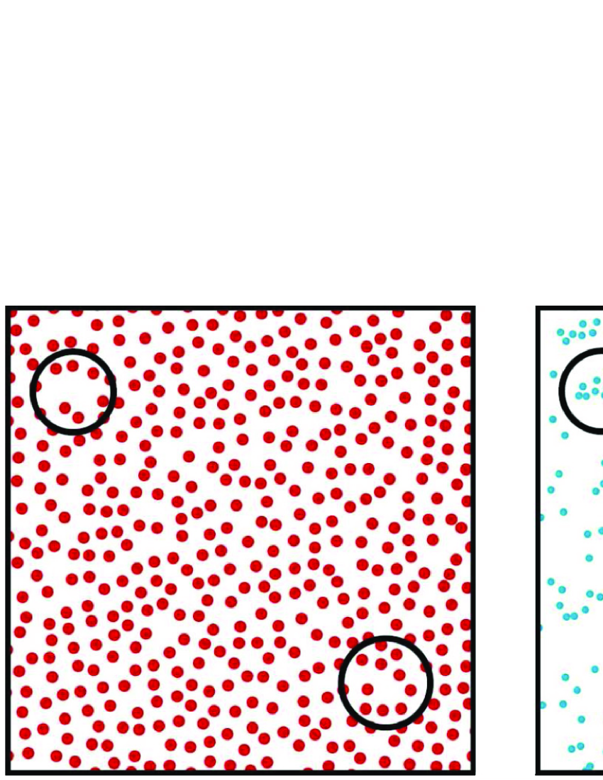
Figure 2: Snapshot of a particle configuration $(\Gamma=5$, relative concentration $\xi=41\%)$ where big (left) and small (right) particles are displayed separately. The clusters of small particles (right) fit in the voids formed by the big particles (left) as highlighted by circles for two examples.

Minkowski functionals provide morphological measures for characterization of size, shape, and connectivity of spatial patterns in $d$ dimensions hadwiger . These functionals turned out to be an appropriate tool to quantify clustering substructures in astronomy, e.g. from galaxies euler2 . They also give insight into the morphology of random interfaces in microemulsions euler1 .
The scalar Minkowski valuations $V$ applied to patterns $P$ and $Q$ in Euclidian space are defined by three types of covariances euler2 :

1. Invariance to motion;

2. Additivity: $V(P\bigcup Q)=V(P)+V(Q)-V(P\bigcap Q)$;

3. Continuity: continuous change for slight distortions in pattern P.

It is guaranteed by the theorem of Hadwiger that in $d$ dimensions there are exactly $d+1$ morphological measures $V$ that are linearly independent hadwiger . For $d=2$, the three functionals have intuitive correspondences: The surface area, the circumference of the surface area, and the Euler characteristic $\chi$.
In two dimensions the Euler characteristic $\chi$ for a pattern $P$ is defined as

$$\chi=S-H$$ (2)

where $S$ is the number of connected areas and $H$ the number of holes.
Morphological information can also be obtained from particle configurations. As configurations only consist of a set of coordinates, a cover disc with radius $R$ is placed on each coordinate to construct a pattern that can be evaluated.
The Minkowski measures are then determined for different cover radii $R$, leading to a characteristic curve for a given configuration, explained in the following (for better understanding follow curves in Figure 3)
The first Minkowski measure (disc area normalized to total area) increases from $0\%$ to $100\%$ for increasing radius $R$ with a decreasing slope when discs start to overlap. The second Minkowski measure (circumference) increases with cover radius $R$, reaches a maximum, and then decays to zero when all holes are overlapped. The third Minkowski measure (Euler characteristic) is very subtle and describes the connection of cover discs and the formation of holes. It allows the most detailed interpretation of a given configuration.
A typical devolution of an Euler characteristic $\chi/N$ with N particles can be divided in three characteristic parts for continuously increasing cover disc radius $R$:

1. For small $R$ the curve is constant at $\chi/N=1$ (normalized to the number of particles $N$). Discs are not touching and thus $S$ is equal to the number of particles. No holes are present. As $\chi$ is normalized with the number of points, the Euler characteristic amounts to $\chi/N=1$.

2. With increasing $R$ the curve drops and $\chi/N$ can become negative when cover discs are large enough to overlap and holes are formed. Therefore, the number of connected areas $S$ decreases and holes are forming which further decreases $\chi/N$. The minimum is reached when discs are connected to a percolating network and the maximum number of holes has formed.

3. For large $R$ the curve starts to raise again because the holes are collapsing until the whole plane is covered with overlapping discs and $\chi/N\rightarrow 0$ for $R\rightarrow\infty$.

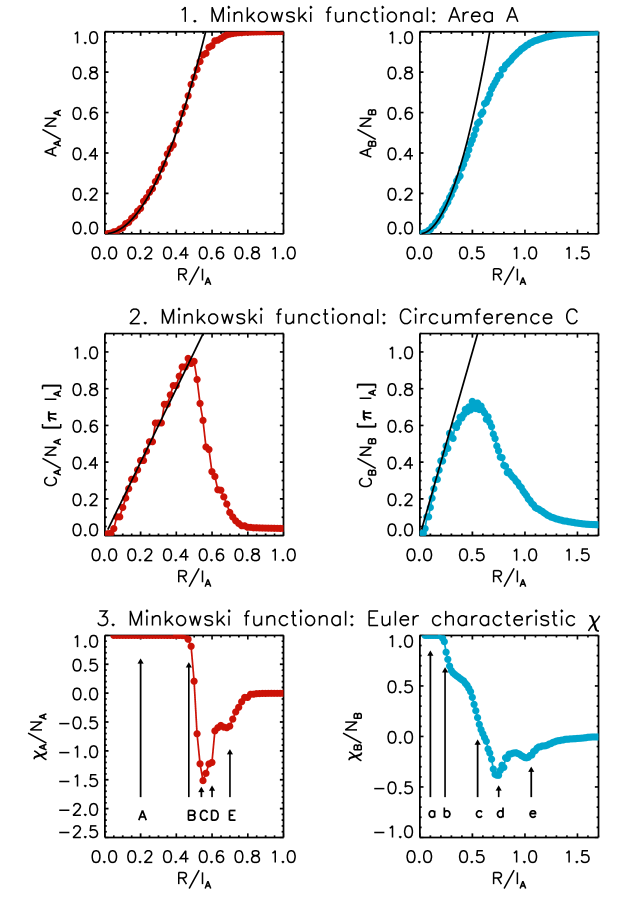
Figure 3: The three ’Minkowski’ measures in 2D (’area’, ’circumference’, and ’Euler characteristic’) are shown for a sample with $\xi=42\%$ at $\Gamma$=662, separately for big (left graphs) and small particles (right graphs). Configurations were decorated with discs and the ’Minkowski’ measures are calculated in dependence on their radius $R/l_{A}$. The solid lines correspond to the ’Minkowski’ measures of a single cover-disc. Marks A-E and a-e in the bottom graphs correspond to radii of interest, and an example of a representative configuration at these labels is displayed in Figure 4. The features of all measures confirm the clustering scenario.

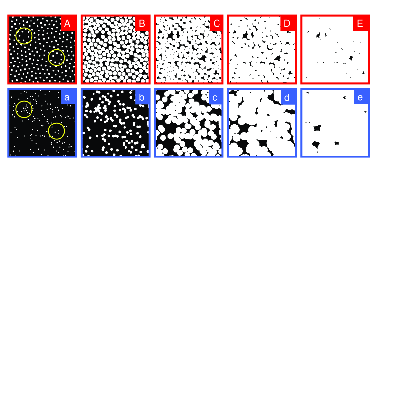
Figure 4: The same section ($375\times 375\,\mu m^{2}$) of a single particle configuration with cover-discs is shown several times in the pictographs A-E and a-e with increasing radius. Pictures correspond to certain radii of interest marked by arrows in the corresponding graphs of the ’Euler characteristic’ in Figure 3. In the first (second) row, just the big (small) particles of this particular configuration are shown. Voids in the big particle configurations are filled with clusters of small particles (examples are highlighted with circles in pictograph ’A’ and ’a’ respectively). Configurations were obtained from a sample with $\xi=42\%$ at $\Gamma=662$.

This qualitative behavior is typical for configurations in 2D. However, the individual morphological information is obtained from specific features in the three regions as the onset of the fall and raise, characteristic kinks or plateaus, and the slope of the fall and raise. The Minkowski measures in dependence on an increasing cover disc provide a characteristic morphological ’fingerprint’ of configurations and therefore statistical evidence of the clustering scenario, complementary to structure factors cluster_prl ; cluster_pre . The statistical noise of the curves is remarkably small compared to that of structure factors as the whole statistical information of a configuration is contained in every data point. Thus, even small features in the curves are true evidence for morphological particularities.
All three Minkowski measures in 2D, area, circumference, and Euler characteristic, are averaged over $100$ configurations for a given temperature and no time-dependence was found during this period of about half an hour. The curves are plotted separately for both species in Figure 3 in dependence on the cover-disc radius. Corresponding snapshots are displayed in Figure 4 to illustrate characteristic radii as indicated. The used sample was strongly supercooled ($\Gamma=662$, $\xi=42\%$), i.e. it was not in equilibrium. However, the features found at these high interaction strengths are the same as for low $\Gamma$, where the sample is in equilibrium. The high interaction strength is used here, as the discussed features become clearer, but it is assumed in the following that the conclusions on clustering are also valid for low interaction strengths $\Gamma$. This assumption will be justified when the dependency on interaction strength is discussed in section 5.
First Minkowski measure: Area
The upper graphs of Figure 3 show the area per particle in dependence on the cover-radius $R/l_{A}$. The covered area starts at zero and is increased continuously to $100\%$ when the discs completely overlap the area. The solid line in both plots indicates the area fraction covered by non-touching free discs. The deviation of the first Minkowski measure from that line shows how homogeneous a configuration is. A clear difference is found between particle species: The big particles follow this reference line up to $\approx 80\%$. This is close to the maximum possible value for hard discs between $84\%$ and $90.7\%$ for random close packing and hexagonal close packing respectively bayer_2d_mct ; random_close ; random_close2 . Therefore, the big particle configurations are very homogeneously distributed. However, the small particles curve deviates from the free disc reference much earlier at $\approx 40\%$ indicating that small particles are much less evenly spread, i.e. they form clusters.
Second Minkowski measure: Circumference
The middle graphs show how the circumference depends on the radius. The black reference line corresponds to a free expanding circle. The measure of the big particles follows this reference line up to $R/l_{A}\approx 0.5$ and then sharply decreases. Again, this is due to the homogeneous distribution of the big particles. Their cover-discs can expand freely up to the maximum possible value of $R_{max}/l_{A}=1/2$ for square order. The measure of the small particles deviates much earlier and less steeply as their particle density is very heterogeneous, i.e. clustered.
Third Minkowski measure: Euler Characteristic
The most detailed information on morphology is obtained from the Euler characteristic. It exhibits many features related to characteristic structures of the investigated configurations. For better understanding of the features described in the following, Figure 4 shows snapshots of a typical section in the used configuration for specific cover-radii. The notation $A-E$ for the big particles and $a-e$ for the small ones is used in both Figures. In Figure 4a and 4A two clusters are highlighted. Firstly, we consider only the big particles. The Euler characteristic $\chi_{A}$ per particle is 1 as the expanding discs are not touching for small radii (mark A). Again, this continues up to a value close to $R/l_{A}\approx 0.5$. The characteristic deviation of all three measures at this same radius states the homogeneity of the big particle distribution. Then, discs touch and $\chi_{A}/N_{A}$ decreases rapidly because surfaces are connecting and holes are forming (mark B). The minimum is reached at mark C, and the Euler characteristic immediately raises because the smallest holes between the triangular close packed regions collapse as seen in the comparison of Figures 4C and 4D. The next holes to collapse are those where one small isolated particle is located. Therefore, a little kink is visible at mark D since these one-particle holes are a little larger than the holes decaying at mark C and therefore ’survive’ a little longer. When they collapse, the Euler characteristic increases rapidly to a pronounced plateau. Note, this plateau is the only statistical evidence for the voids in the big particle configuration made up by the clusters: these voids are large and thus they ’survive’ for a long ’time’ resulting in that plateau. These voids are not detectable with the other Minkowski measures or the static structure factor of the big particles cluster_prl ; cluster_pre . Finally, they start to decay at mark E, but not suddenly, which shows that they have a distribution in size.
The Euler characteristic of the small particles shows the complementary picture: Starting with low values of $R/l_{A}$ the characteristic is $\chi_{B}/N_{B}=1$ for free disc expansion. The first drop at mark b occurs at much lower values than for the big particles because small particles in clusters connect. The subsequent shoulder right next to mark b confirms the clustering: small particles inside a cluster are now connected, and it needs some further increase of disc radius until the clusters themselves start connecting. A small second shoulder at mark c originates from the isolated particles that are not arranged in clusters. They are the last particles incorporated until all discs form a percolating network at the minimum at mark d. The increase of $\chi_{B}/N_{B}$ shows how the holes are closing. While the increase in the Euler characteristics of the big particles has a plateau at mark E, the small particles have a clear dip at mark e. This reveals information on the shape of the clusters: The voids in the big particle positions are compact in shape stopping the increase of the Euler characteristic before mark E. In contrast, the small particles arrange in chain-like clusters. When the voids between these structures close, they decay into several sub-holes causing the characteristic to decrease again. In fact, the big particles also cause a little dip at their plateau for the voids can sometimes also decay into sub-holes. However, this dip is much smaller than for the small ones.
Most features are also visible in the Euler characteristic obtained from Brownian dynamics simulation cluster_prl . There, the same qualitative behavior is found but the smaller features are ’washed out’ because the used interaction strengths were much lower, as discussed in the following section. Further, the variation of the relative concentration $\xi$ and the subsequent dependence of the features in the Euler characteristic will confirm the interpretation of the scenario.

5 Dependence of clusters on interaction strength and relative concentration

Figure 5: Fraction of small particles (relative to all small particles $N_{S}$, left axis) that are arranged in clusters. This fraction is independent of $\Gamma$ but dependent on relative concentration $\xi$. The dashed lines correspond to the average fractions over all interaction strengths $\Gamma$.
Solid squares represent the fraction of small particles (relative to all small particles $N_{S}$, right axis) that are arranged in square symmetry as evaluated in epje_ebert .

In order to demonstrate the connection between clustered equilibrated fluid and supercooled local crystalline structure, the dependence of partial clustering on the interaction strength $\Gamma$ and on the average relative concentration $\xi$ is now discussed.
In Figure 5 the fraction of small particles arranged in clusters is plotted versus interaction parameter $\Gamma$ for two different relative concentrations $\xi$. A small particle is characterized as ’cluster-particle’, when the closest neighbor is also a small particle. This simple criteria implies that the smallest possible cluster consists of two close small particles surrounded in a cage of big ones. In the graph of Figure 5 for $\xi\approx 43\%$ it is found that a high fraction of $\approx 80\%$ of all small particles is arranged in clusters. Even for a lower relative concentration $\xi\approx 29\%$, still $\approx 65\%$ are arranged in clusters. Note, that the fraction of small particles in both samples is smaller than that of the big particles as $\xi<0.5$. Therefore, every small particle could have enough possibilities to arrange far away from the next small particle which is obviously not the case. For an arbitrary distribution of the small particles over the number of possible sites (which is equal to the number of big particles) a fraction of $40\%$ is expected for a relative concentration $\xi=29\%$ and a fraction of $55\%$ for a relative concentration $\xi=43\%$ . The fact that these expected values are significantly lower than the actually measured ones additionally confirms that small particles effectively attract each other and therefore cluster.

The main result from Figure 5 for the structure of this colloidal glass former is that the fraction of cluster-particles is independent of the interaction parameter $\Gamma$, in contrast to local crystallinity which strongly increases upon supercooling: Clusters do not vanish although the local structure is dominated by local crystallinity for strong supercooling epje_ebert . This is demonstrated for the example of square order in the same Figure 5 (for details see epje_ebert ).
The local relative concentration is frozen in. Small particles are not redistributed to match an equilibrium crystal structure which would reduce the number of cluster-particles (e.g. in square order). In fact, the independence of the clustering from $\Gamma$ shows that the opposite is the case: The clusters force the local structure into that crystalline order which matches best with the local relative concentration. In this way, local crystallinity is established without long-range order epje_ebert as it inherits the clustered distribution of the small particles.

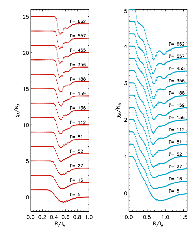
Figure 6: ’Euler characteristics’ of big (left) and small (right) particles for different interaction strengths $\Gamma$. Characteristic features are visible for the lowest $\Gamma$ and become clearer with increasing $\Gamma$. The relative concentration was $\xi\approx 43\%$. Curves are shifted for reasons of clarity.

This behavior is confirmed by the graphs of Figure 6. The Euler characteristics for both species are plotted over a wide range of the interaction strength $\Gamma$, from fluid $(\Gamma=5$) to the strongly supercooled state $(\Gamma=662$): the curves change continuously. The main clustering features as discussed in Figure 4 are visible for all values of $\Gamma$, they just become sharper with increasing interaction strength. The smallest features like the kink at mark D in Figure 3 are smeared out for low $\Gamma$ but the plateaus and shoulders characterizing the partial clustering are qualitatively independent of $\Gamma$.

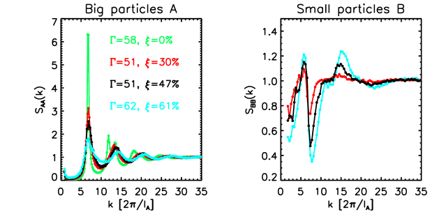
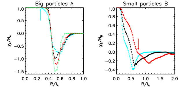
Figure 7: Static structure factors and ’Euler characteristics’ of samples with comparable interaction strength $\Gamma$ but different relative concentration $\xi$. Indicated values for $\Gamma$ and $\xi$ are valid for all graphs.
Upper graphs: Static structure factors for big (left) and small particles (right). With increasing relative concentration of small particles the features of $S_{BB}(k)$ gain more contrast, and peaks in the $S_{AA}(k)$ are shifted slightly towards higher k-values.
Lower graphs: ’Euler characteristics’ for big (left) and small particles (right). For decreasing $\xi$ the minimum in $\chi_{B}/N_{B}$ is shifted towards larger radii $R$. The weight of the features changes, e.g. the last shoulder in the drop in $\chi_{B}/N_{B}$ (red arrow, right plot). This shoulder results from the incorporation of isolated small particles into the network (see Figure 3) and is only visible for the lowest relative concentration $\xi=30\%$ (red curve) at this interaction strength $\Gamma$. The blue arrow in the bottom left plot marks the onset of the inter-particle connection of the big particles for the sample with highest relative concentration $\xi=61\%$. The onset is shifted to a lower value $R$ compared to the other curves.

In Figure 7 the dependence of the local structure on relative concentration $\xi$ is shown using structure factors and Euler characteristics. There, samples with comparable interaction strengths $\Gamma$ but different relative concentrations $\xi$ are compared. Adding small particles is shifting the peaks of the structure factor $S_{AA}(k)$ towards higher $k$-values. This can be understood by the clustering effect: Small particles form clusters and push the big particles closer together resulting in a shift of the main peak. This shift is small for the used parameters. However, confirmation of this interpretation is found in cluster_pre where Liquid integral equation theory shows the same result unambiguously. There, parameters were used that are not accessible in the experiment (different ratios of the magnetic moments $\chi_{B}/\chi_{A}$). The contrast in $S_{BB}(k)$ is increased for higher relative concentrations $\xi$ which is also in agreement with theory cluster_pre .
The Euler characteristics for the same samples, shown in the lower graphs of Figure 7, confirm this interpretation. The drop in the $\chi_{A}/N_{A}$ (bottom left) becomes deeper when less small particles are present. Then, the distances between big particles are less distributed due to fewer clusters. The increase becomes steeper for the same reason: clusters of small particles cause larger voids collapsing at higher cover-disc radii. It is remarkable, that the onset of the steep drop is earlier for high relative concentrations ($\xi=61\%$, blue curve) as indicated by the blue arrow. Again, this is caused by the small particle clusters that push together the big particles.
A strong dependence is found in the Euler characteristics of the small particles: the onset of the first drop is independent on the relative concentration indicating that the local density of particles in clusters is not affected (unlike that of the big ones). What significantly changes is the depth of the first drop. The more small particles, the deeper the drop, because more small particles are arranged in clusters. The last shoulder, before the Euler characteristic reaches its minimum (marked by red arrow), refers to the isolated particles (see section 4). Therefore, at these interaction strengths this shoulder is only visible for the sample with the lowest relative concentration $\xi=30\%$ (red curve) which has the most isolated particles (compare also with Figure 5).
The systematic dependence of Euler characteristics and static structure factors on relative concentration $\xi$ confirms the interpretation of partial clustering of section 4. However, the main result of this section is that the principle occurrence of the effect is independent of the interaction strength: The clustering in equilibrium at low interaction strengths is therefore responsible for the variety of local crystallinity at strong supercooling suppressing long-range order epje_ebert .

6 Conclusions

On a local scale the system reveals the non-trivial ordering phenomenon of partial clustering: the small particles tend to form loose clusters while the big particles are homogeneously distributed. The origin of this effect is traced back to the negative nonadditivity of the dipolar pair potential. The detailed scenario is quantified using Minkowski functionals applied to experimentally obtained configurations. Changing the interaction strength $\Gamma$ reveals that the principle scenario does not qualitatively depend on the interaction strength, and, as a consequence, the local relative concentration is simply ’frozen’ in. However, the strength of the effect increases with the relative concentration $\xi$.
The clustering effect together with the missing ability of the system to reorganize fast enough into an equilibrated state (i.e. extended crystal structure epje_ebert ; dipolar_crystals ; gen_algorithm ) is crucial to understand the glass forming behavior of this system: The partial clustering leads locally to a heterogeneous relative concentration $\xi$ which then leads for increasing interaction strengths $\Gamma$ to local crystallinity epje_ebert without long-range order. It provides the necessary complexity for glassy frustration in this 2D system and prevents solidification into the energetically preferred crystalline or poly-crystalline morphologies dipolar_crystals ; gen_algorithm .

This work was supported by the Deutsche Forschungsgemeinschaft SFB 513 project B6, SFB TR 6 project C2 and C4 and the International Research and Training Group ”Soft Condensed Matter of Model Systems” project A7. We thank P. Dillmann for fruitful discussion and experimental contributions.

References

-
(1)
N. Hoffmann, F. Ebert, C. Likos, H. Löwen, G. Maret, Phys. Rev. Lett. 97,
078301 (2006). - (2) B. I. Halperin, D. R. Nelson, Phys. Rev. Lett. 41, 121 (1978).
- (3) K. Zahn, G. Maret, Phys. Rev. Lett. 85, 3656 (2000).
- (4) P. Keim, G. Maret, H. H. von Grünberg, Phys. Rev. E 75, 031402 (2007).
- (5) L. Onsager, Phys. Rev. 65, 117 (1944).
- (6) H. König, R. Hund, K. Zahn, G. Maret, Eur. Phys. J. E 18, 287 (2005).
- (7) D. Perera, P. Harrowell, Phys. Rev. E 59, 5721 (1999).
- (8) M. Bayer, J. Brader, F. Ebert, M. Fuchs, E. Lange, G. Maret, R. Schilling, M. Sperl, J. Wittmer, Phys. Rev. E 76, 011508 (2007).
- (9) F. Ebert, P. Keim, G. Maret, Eur. Phys. J. E 26, 161 (2008).
- (10) J. H. Conway, S. Torquato, Proceedings of the National Accademy of Science 103 No. 28, 10612 (2006).
- (11) H. J. Schöpe, G. Bryant, W. van Megen, Phys. Rev. Lett. 96, 175701 (2006).
- (12) M. D. Rintoul S. Torquato, Phys. Rev. Lett. 77, 4198 (1996).
- (13) S. R. Williams, I. K. Snook, W. van Megen, Phys. Rev. E 64, 021506 (2001).
- (14) P. N. Pusey J. Phys.: Condens. Matter 20, 494202 (2008).
-
(15)
T. Mizuguchi, T. Odagaki, M. Umezaki, T. Koumyou, J.
Matsui, CP982 - Complex Systems, 5th international Workshop
on Complex Systems,
234 (2008). - (16) H. Shintani, H. Tanaka, Nature Physics 2, 200 (2006).
- (17) T. Kawasaki, T. Araki, H. Tanaka, Phys. Rev. Lett. 99, 215701 (2007).
- (18) M. Leunissen, C. Christova, A. Hynninen, C. Royall, A. Campbell, A. Imhof, M. Dijkstra, R. van Roij, A. van Blaaderen, Nature 437, 235 (2005).
- (19) L. Assoud, R. Messina, H. Löwen, Eur. Phys. Lett. 80, 48001 (2007).
- (20) J. Fornleitner, F. Lo Verso, G. Kahl, C. N. Likos, Soft Matter 4, 480 (2008).
- (21) N. Hoffmann, C. Likos, H. Löwen, J. of Phys.: Cond. Mat. 18, 10193 (2006).
- (22) F. Ebert, P. Dillmann, G. Maret, P. Keim, arXiv:0903.2808 (2009).
- (23) A. Buhot, W. Krauth, Phys. Rev. E 59, 2939 (1999).
- (24) H. Hadwiger, Vorlesungen über Inhalt, Oberfläche und Isoperimetrie, Springerverlag, Berlin (1957).
-
(25)
C. Beisbart, R. Valdarnini, T. Buchert, Astronomy Astrophysics 379,
412 (2001). - (26) C. N. Likos, K. R. Mecke, H. Wagner, J. Chem. Phys. 102, 9350 (1995).
- (27) J. Berryman, Phys. Rev. A 27, 1053 (1983).
-
(28)
T. S. Majmudar, M. Sperl, S. Luding, R. P. Behringer, Phys. Rev. Lett. 98,
058001 (2007).