Cooperative Transmission in a Wireless Relay Network based on Flow Management

Abstract

In this paper, a cooperative transmission design for a general multi-node half-duplex wireless relay network is presented. It is assumed that the nodes operate in half-duplex mode and that channel information is available at the nodes. The proposed design involves solving a convex flow optimization problem on a graph that models the relay network. A much simpler generalized-link selection protocol based on the above design is also presented. Both the proposed flow-optimized protocol and the generalized-link selection protocol are shown to achieve the optimal diversity-multiplexing tradeoff (DMT) for the relay network. Moreover, simulation results are presented to quantify the gap between the performances of the proposed protocols and that of a max-flow-min-cut type bound, in terms of outage probability.

I Introduction

A wireless relay network is one in which a set of relay nodes assist a source node transmit information to a destination node. Practically the wireless nodes can only support half-duplex communication [1], i.e., no nodes can receive and transmit information simultaneously on the same frequency band. Different cooperative transmission schemes for systems with half-duplex nodes have been proposed in the literature. Fundamentally, these schemes consist of two basic steps. First, the source transmits to the destination, and the relay listens and “captures” [2] the transmission from the source at the same time. Next, the relays send processed source information to the destination while the source may still transmit to the destination directly. Variants of these techniques have been proposed and have been shown to yield good performance under different circumstances [4, 3, 1].

Assuming channel state information (CSI) at the nodes, an opportunistic decode-and-forward (DF) protocol for half-duplex relay channels is proposed in [5]. In [6], the authors present routing algorithms to optimize the rate from a source to a destination, based on the DF technique that uses regular block Markov encoding and windowed decoding [7, 8], for the Gaussian full-duplex multiple-relay channel. The achievable rate of [7] for the Gaussian physically degraded full-duplex multi-relay channel has been established as the capacity of this channel in [9]. In [10], it is shown that the cut-set bound on the capacity of the Gaussian single source-multiple relay-single destination mesh network can be achieved using the compress-and-forward (CF) method, as the relay powers go to infinity.

Some simpler cooperative diversity methods based on network path selection have been recently reported [11, 12]. These selection methods include: (i) the max-min selection method [11], wherein the relay node with the maximum of the minimum of the source-relay and relay-destination channel gains is selected; (ii) the harmonic mean selection method [11], wherein the relay node with the highest harmonic mean of the source-relay and relay-destination channel gains is selected; and (iii) the selection scheme of [12], in which the relay that can correctly decode the information from the source and has the best relay-destination channel is selected. These methods achieve a DMT of $d(r)=(N-1)(1-2r)$ for an $N$ node relay network and multiplexing gain $0<r<0.5$. This is close to what the distributed space-time coding protocol [13] achieves, when $N$ is large. Unfortunately, these network selection protocols perform poorly in high-rate scenarios ($r>0.5$).

We have proposed a cooperative diversity design based on a flow optimization approach for a three-node network in [14]. In this design, the source node broadcasts two distinct flows to the destination and the relay node respectively during the relay’s listen period. Then the relay forwards this information using the DF approach while the source may also send another flow of information to the destination during the relay’s transmit period. This scheme is shown to achieve the optimal diversity order for the three-node relay channel and yield performance very close to optimal full-duplex relaying in both low- and high-rate situations.

Here, we apply this cooperative transmission design to a general relay network, wherein wireless links are present between each pair of nodes in the network. As in [14], assuming CSI is available at all nodes we use broadcasting (BC), multiple access (MA) and time sharing (TS) techniques to formulate a flow theoretic convex optimization problem based on the channel conditions. Instead of considering a total power constraint for all the transmitting nodes as in [14], we subject each node to a maximum transmit power constraint. This yields a more reasonable system model for a general wireless relay network, especially when the number of nodes in the relay network is large. The resulting relaying protocol will be referred to as the flow-optimized (FO) protocol. To obtain a more practical cooperative design we develop a generalized-link selection (GLS) protocol, in which we select the best relay node out of the available ones to form an equivalent three-node relay network to transmit the information from the source to the destination. The benefit of this, over other network path selection strategies, becomes evident when the rate requirement is high. It is shown that the simple GLS protocol is optimal in terms of the DMT [15] and yields acceptable performance even when the rate requirement is high.

Recently, in [16], the authors have shown that compress-and-forward (CF) relaying achieves the optimal DMT for the three-node, half-duplex network, and that DF relaying can achieve the optimal DMT of the four-node full-duplex network. In this work, we show that the optimal DMT can be achieved for a general $N$-node ($N\geq 3$) half-duplex network using the FO or GLS protocols. Here, it should be clarified that we consider that the wireless links between each node-pair experience independent Rayleigh fading, and this corresponds to the definition of non-clustered networks in [16]. The performances of the FO and GLS protocols are evaluated numerically in terms of their outage probabilities for four- and five-node relay networks for uniform and non-uniform average power gains. The numerical results motivate the use of the GLS protocol for situations where computation complexity is an issue and show a remarkable improvement over the max-min selection method of [11]. The proposed designs, based on BC and MA alone, are sub-optimal in general. For a fair appraisal of the proposed protocols, we compare the proposed protocols to an upper bound on the maximum rate, derived using the max-flow-min-cut theorem [17, Thm. 14.10.1].

II A General Design Using A Flow-theoretic Approach

We consider an $N$-node wireless relay network with a link joining each pair of nodes. Each such wireless link is described by a bandpass Gaussian channel with bandwidth $W$ and one-sided noise spectral density $N_{0}$. We denote the power gain of the link from node $i$ to node $j$ as $Z_{ij}$. The link power gains are assumed to be independent and identically distributed (i.i.d.) exponential random variables with unit mean. This corresponds to the case of independent Rayleigh fading channels with unit average power gains. Moreover, we assume that each node has a maximum power limit of $P$ and can only support half-duplex transmission. Note that this model can be easily generalized to the case where channels may have non-uniform average power gains (for which numerical examples are presented in Section IV), and where different nodes may have different maximum power constraints. More specifically, the latter case can be converted into the uniform maximum power constraints case by absorbing the non-uniformity in the transmit powers into the average power gains of the corresponding links. In the sequel, we characterize the system in terms of the transmit signal-to-noise ratio (SNR), $S=\frac{P}{N_{0}W}$, at the input of the links. Time is divided into unit intervals, and BC and MA are applied with a TS strategy that is optimized to maximize the spectral efficiency (which we call “rate” hereafter for convenience). To avoid interference between concurrent transmissions, a time interval is divided into slots:

• During the first slot, the source may BC to all the other nodes in the network.

• During the subsequent slots, a relay may BC to all other nodes (except the source node), or it may receive flows from all other nodes (except from the destination) through MA.

• During the very last slot, the source and the relays may send information flows to the destination using MA.

Note that the forwarding of information by the relays is based on the DF approach. For practicality consideration, it is assumed that the phases of the simultaneously transmitted signals from different nodes are not synchronized. In general, for the above transmission protocol, there would be a maximum of $2(N-2)+2=2N-2$ time slots of lengths $t_{1},t_{2},\cdots,t_{2N-2}$ respectively.

Next, we describe the optimization problem using a graph-theoretic formulation. Define a graph $G=(V,E)$, where $V$ is the set of nodes, $E$ is the set of all links joining the nodes in the graph, and associate the vector $\underline{r}$ to represent the flow rates associated with each link in $E$. Thus, the number of elements in $\underline{r}$ equals the cardinality of $E$. For convenience, we write $G=(V,E,\underline{r})$. Now denote the source by $\mathcal{S}$, the destination by $\mathcal{D}$, and the relay nodes by $\mathcal{R}_{1},\ldots,\mathcal{R}_{N-2}$. The slotting of a unit time interval, as described above, yields simpler graphs for each time slot, that we call basic graphs. A basic graph is either one in which a particular node may BC to several nodes, or in which several nodes transmit via MA to a particular node. Thus for a basic graph, we need to include only the links between the nodes that may participate during the concerned time slot. For example, assume that the relay $\mathcal{R}_{1}$ broadcasts to all nodes other than the source, during the $i$-th time slot. The basic graph is given by $G_{i}=(V,E_{i},\underline{r}_{i})$ where $V=\{\mathcal{S},\mathcal{R}_{1},\cdots,\mathcal{R}_{N-2},\mathcal{D}\},~{}E_{i}=\{\mathcal{R}_{1}\mathcal{R}_{2},\cdots,\mathcal{R}_{1}\mathcal{R}_{N-2},\mathcal{R}_{1}\mathcal{D}\},~{}\underline{r}_{i}=\left(\frac{x_{\mathcal{R}_{1}\mathcal{R}_{2}}^{i}}{t_{i}}~{}\cdots~{}\frac{x_{\mathcal{R}_{1}\mathcal{R}_{N-2}}^{i}}{t_{i}}~{}\frac{x_{\mathcal{R}_{1}\mathcal{D}}^{i}}{t_{i}}\right)^{T}$, where $x_{AB}^{i}$ is the flow from node $A$ to node $B$ during the $i$-th time slot.

In general, the proposed design involves TS between the basic graphs to yield the following equivalent graph $G$ corresponding to a unit interval (see [18] for a similar idea):

$$G=\left(V,~{}\bigcup_{i}E_{i},~{}\sum_{i}t_{i}\underline{r}_{i}\right)=t_{1}G_{1}+t_{2}G_{2}+\ldots+t_{2N-2}G_{2N-2}.$$ (1)

where the number of elements in each vector $\underline{r}_{i}$ is extended to $|\bigcup_{i}E_{i}|$ by inserting zeros appropriately. The second equality in (1) implies that $G$ can be viewed as a linear combination of the basic graphs $G_{i}$s, with the equivalent set of edges given by the union of the sets $E_{i}$, and the equivalent flow rate vector given by the linear combination of the individual flow rate vectors $\underline{r}_{i}$.

To maximize the data rate from the source to the destination through the relay network, we need to consider each cut that partitions $V$ into sets $V^{s}$ and $V^{d}$ with $\mathcal{S}\in V^{s}$ and $\mathcal{D}\in V^{d}$. Clearly, there can be $2^{N-2}$ such possible cuts for the $N$-node relay network. Let these cuts and the corresponding cut sets be denoted by $\mathcal{C}_{k}$, $V^{s}_{k}$, and $V^{d}_{k}$, respectively, for $k=1,2,\cdots,2^{N-2}$. Further, for the graph $G$, for any two nodes $A\in V^{s}_{k}$ and $B\in V^{d}_{k}$, there exists a cut edge $AB$ that crosses the cut. Denote the total flow through cut edge $AB$ in a unit time interval by $x_{AB}=\sum_{i=1}^{2N-2}x_{AB}^{i}$. Now recall from network flow theory [19] that the maximum flow rate from the source to the destination is specified by the minimal cut of the equivalent graph (1). Consequently, we arrive at the following convex flow optimization problem that can be solved using standard optimization techniques:

$$\max\min\left(\sum_{A\in V^{s}_{1},B\in V^{d}_{1}}x_{AB},\sum_{A\in V^{s}_{2},B\in V^{d}_{2}}x_{AB},\cdots,\sum_{A\in V^{s}_{2^{N-2}},B\in V^{d}_{2^{N-2}}}x_{AB}\right)$$ (2)

over all flow allocations $x_{AB}^{i}$ and all time slot lengths $t_{i}$, subject to

• the non-negativity constraints: $x_{AB}^{i}$, $t_{i}\geq 0$ for all cut edges $AB$ and $i=1,2,\cdots,2N-2$,

• the total-time constraint: $t_{1}+\ldots+t_{2N-2}=1$,

• the power (capacity) constraints:

  • for a BC slot the flow rates should lie in the capacity region of the BC channel with the transmitting node having a power constraint of $P$,

  • for an MA slot the flow rates should lie in the capacity region of the MA channel with a maximum power constraint $P$ for each transmitting node,

• the flow constraints: considering steady state operation, the total information flow out of a relay should equal the flow into the relay in each unit time interval.

Note that the dependence of the objective function on the channel gains and the time slot lengths is implicitly expressed through the capacity constraints. Denote the cut separating $\mathcal{S}$ from all the other nodes and the cut separating $\mathcal{D}$ from all nodes as $\mathcal{C}_{\mathcal{S}}$ and $\mathcal{C}_{\mathcal{D}}$, respectively. Then we observe that the cost function in (2) above can be further simplified to $\max~{}\min\left\{x(\mathcal{C}_{\mathcal{S}}),~{}x(\mathcal{C}_{\mathcal{D}})\right\}$, where

$$x(\mathcal{C}_{\mathcal{S}})=x_{\mathcal{SD}}+\sum_{j=1}^{N-2}x_{\mathcal{S}\mathcal{R}_{j}}\mathrm{~{}~{}~{}and~{}~{}~{}}x(\mathcal{C}_{\mathcal{D}})=x_{\mathcal{SD}}+\sum_{i=1}^{N-2}x_{\mathcal{R}_{i}\mathcal{D}}$$ (3)

are the total flows across the above-mentioned cuts $\mathcal{C}_{\mathcal{S}}$ and $\mathcal{C}_{\mathcal{D}}$, respectively. To see this, consider the cut $\mathcal{C}$ with $V^{s}=\{\mathcal{S},\mathcal{R}_{1},\cdots,\mathcal{R}_{l}\}$, and $V^{d}=\{\mathcal{R}_{l+1},\cdots,\mathcal{R}_{N-2},\mathcal{D}\}$ for some $l\in\{1,2,\cdots,N-2\}$. The total flow across this cut is given by

$$x(\mathcal{C})=x_{\mathcal{SD}}+\sum_{j=l+1}^{N-2}x_{\mathcal{S}\mathcal{R}_{j}}+\sum_{i=1}^{l}\left(x_{\mathcal{R}_{i}\mathcal{D}}+\sum_{j=l+1}^{N-2}x_{\mathcal{R}_{i}\mathcal{R}_{j}}\right).$$ (4)

Now, consider node $i$ for $i\in\{1,2,\cdots,l\}$. According to the flow constraint for node $i$,

$$x_{\mathcal{R}_{i}\mathcal{D}}+\sum_{j=l+1}^{N-2}x_{\mathcal{R}_{i}\mathcal{R}_{j}}+\sum_{k=1,k\neq i}^{l}x_{\mathcal{R}_{i}\mathcal{R}_{k}}=x_{\mathcal{S}\mathcal{R}_{i}}+\sum_{j=l+1}^{N-2}x_{\mathcal{R}_{j}\mathcal{R}_{i}}+\sum_{k=1,k\neq i}^{l}x_{\mathcal{R}_{k}\mathcal{R}_{i}}.$$ (5)

Summing (5) over all $i\in\{1,2,\cdots,l\}$ we get

$$\sum_{i=1}^{l}\left(x_{\mathcal{R}_{i}\mathcal{D}}+\sum_{j=l+1}^{N-2}x_{\mathcal{R}_{i}\mathcal{R}_{j}}\right)=\sum_{i=1}^{l}\left(x_{\mathcal{S}\mathcal{R}_{i}}+\sum_{j=l+1}^{N-2}x_{\mathcal{R}_{j}\mathcal{R}_{i}}\right).$$ (6)

Since $\sum_{i=1}^{l}\sum_{j=l+1}^{N-2}x_{\mathcal{R}_{j}\mathcal{R}_{i}}\geq 0$, combining (3), (4) and (6) gives $x(\mathcal{C})\geq x(\mathcal{C}_{\mathcal{S}})$. Similarly, we have $x(\mathcal{C})\geq x(\mathcal{C}_{\mathcal{D}})$. Thus the cost function in (2) reduces to the above-mentioned form.

III Generalized-link Selection and Its Optimality

In this section, we present the GLS protocol and establish the optimality of the FO and GLS protocols in terms of the DMT. This is accomplished in three steps. First, we apply the FO protocol to the three-node relay network. Next, we propose the GLS protocol based on a selection strategy that is sub-optimal to the FO protocol of Section II. Finally, the optimality of the GLS protocol, and thereby, that of the FO protocol, is established.

III-A The Three-node Relay Network

The three-node relay network consists of a source ($\mathcal{S}$), a relay ($\mathcal{R}$), and a destination ($\mathcal{D}$). We specialize the general design described in the previous section to this three-node relay network. A unit time interval is divided into two time slots of lengths $t_{1}$ and $t_{2}$ with $t_{1}+t_{2}=1$. During the first time slot, $\mathcal{S}$ sends (via BC) two flows of rates $x_{\mathcal{SD}}^{1}/t_{1}=x_{1}/t_{1}$ and $x_{\mathcal{SR}}^{1}/t_{1}=x_{2}/t_{1}$ to $\mathcal{D}$ and $\mathcal{R}$, respectively, resulting in the basic graph $G_{1}$. During the second time slot, $\mathcal{R}$ and $\mathcal{S}$ send (via MA) two flows of rates $x_{\mathcal{RD}}^{2}/t_{2}=x_{4}/t_{2}$ and $x_{\mathcal{SD}}^{2}/t_{2}=x_{3}/t_{2}$ to $\mathcal{D}$, respectively, resulting in the basic graph $G_{2}$. Combining the two basic graphs yields the equivalent graph as $G=t_{1}G_{1}+t_{2}G_{2}$. Note that the information flow of rate $x_{4}/t_{2}$ sent by $\mathcal{R}$ during the MA time slot is from the flow of rate $x_{2}/t_{1}$ it received during the BC time slot. Thus, we have the flow constraint $x_{4}=x_{2}$. The rate for this network is specified by the min-cut which is clearly $\min\{(x_{1}+x_{2}+x_{3}),(x_{1}+x_{4}+x_{3})\}$. Hence, the flow optimization problem is given by:

$$\max~{}\min~{}\{(x_{1}+x_{2}+x_{3}),(x_{1}+x_{4}+x_{3})\}$$ (7)

over flow allocations $x_{1},~{}x_{2},~{}x_{3},~{}x_{4}$, and time slot lengths $t_{1},~{}t_{2}$, subject to

• non-negativity constraints: $x_{1},x_{2},x_{3},x_{4}\geq 0,\quad t_{1},t_{2}\geq 0$,

• total-time constraint: $t_{1}+t_{2}=1$,

• power constraints: $S_{BC}\leq S,~{}x_{1}\leq t_{1}C(Z_{\mathcal{SD}}S),~{}x_{2}\leq t_{1}C(Z_{\mathcal{SR}}S)$ for the BC slot,
  $\qquad x_{3}\leq t_{2}C(Z_{\mathcal{SD}}S),~{}x_{4}\leq t_{2}C(Z_{\mathcal{RD}}S),~{}x_{3}+x_{4}\leq t_{2}C(Z_{\mathcal{SD}}S+Z_{\mathcal{RD}}S)$ for the MA slot,

• flow constraint: $x_{2}=x_{4}$,

where $C(x)=\log(1+x)$, and $S_{BC}$, the minimum SNR required for the source to broadcast at rates $x_{1}/t_{1}$ and $x_{2}/t_{1}$ to the destination and the relay, respectively, in the first time slot with $0<t_{1}\leq 1$, is given by (see [14, Lemma 3.1] for proof)

$$S_{BC}=\left\{\begin{array}[]{ll}\frac{1}{Z_{\mathcal{S}\mathcal{D}}}(e^{x_{1}/t_{1}}-1)+\frac{1}{Z_{\mathcal{S}\mathcal{R}}}e^{x_{1}/t_{1}}(e^{x_{2}/t_{1}}-1)\mathrm{~{}for~{}}Z_{\mathcal{S}\mathcal{R}}>Z_{\mathcal{S}\mathcal{D}},\\ \frac{1}{Z_{\mathcal{S}\mathcal{R}}}(e^{x_{2}/t_{1}}-1)+\frac{1}{Z_{\mathcal{S}\mathcal{D}}}e^{x_{2}/t_{1}}(e^{x_{1}/t_{1}}-1)\mathrm{~{}for~{}}Z_{\mathcal{S}\mathcal{R}}\leq Z_{\mathcal{S}\mathcal{D}}.\end{array}\right.$$

For $t_{1}=0$, $S_{BC}=0$. Note that for the BC slot, the last two constraints are redundant when $t_{1}>0$, and complements the first constraint when $t_{1}=0$.

The solution of this flow optimization problem is given in Appendix -A. As mentioned in Section I, the above optimization problem formulation is different from that in [14] wherein the sum of the source and relay powers, required to achieve a certain data rate, is minimized. More specifically, when considering individual power constraints for each node, we cannot use part $2$ of [14, Lemma 3.1] to describe the power constraints for the MA slot. This is because doing so would restrict the flows $x_{2}$ and $x_{3}$ such that the sum of powers expended at $\mathcal{S}$ and $\mathcal{R}$ is minimized. On the other hand, in the present problem, the power constraints only dictate that the flow-rates should lie in the MA capacity region specified by the maximum power available at each transmitting node, for the particular fading state. With this modification in the constraint for the MA slot, the solution approach to the above problem needs to be markedly different from that in [14] as shown in Appendix -A. The maximum information rate from the source $\mathcal{S}$ to the destination $\mathcal{D}$ for different cases is summarized below:

a) $Z_{\mathcal{SD}}\geq Z_{\mathcal{SR}}$: The maximum rate is $X(S)=C(Z_{\mathcal{SD}}S)$ with direct transmission from $\mathcal{S}$ to $\mathcal{D}$.

b) $Z_{\mathcal{SD}}<Z_{\mathcal{SR}}$: The maximum rate is $X(S)=\max_{0\leq t_{2}\leq t_{2\textnormal{max}}}t_{1}\log\left(\frac{1+Z_{\mathcal{SD}}S}{1+\frac{Z_{\mathcal{SD}}}{Z_{\mathcal{SR}}}\left[\left(1+\frac{Z_{\mathcal{RD}}S}{1+Z_{\mathcal{SD}}S}\right)^{t_{2}/t_{1}}-1\right]}\right)+t_{2}C(Z_{\mathcal{SD}}S+Z_{\mathcal{RD}}S)$ with $t_{2\textnormal{max}}=C(Z_{\mathcal{SR}}S)/\left[C(Z_{\mathcal{SR}}S)+C(Z_{\mathcal{RD}}S+Z_{\mathcal{SD}}S)-C(Z_{\mathcal{SD}}S)\right]$ and $t_{1}=1-t_{2}$.

Thus for a given power limit (i.e. a given $S$) at the nodes, relaying is advantageous only when $Z_{\mathcal{SD}}<Z_{\mathcal{SR}}$. Further, the optimal solution always allocates a non-zero flow to the direct link. Also, the relay-destination link gain $Z_{\mathcal{RD}}$ does not influence the strategy of transmission (i.e. whether to use only the direct link or both the relay and direct links), but only the amount of information through the relay link.

III-B Generalized-link Selection

For the general $N$-node relay network, the flow optimization solution can be computationally demanding even for moderate values of $N$. The GLS protocol described below provides a simple sub-optimal design to address this complexity issue. In essence, the GLS protocol identifies the best relay path out of the possible $N-2$ relay paths and considers only the chosen relay along with the source and destination to form a three-node relay network, which we call a generalized-link from the source to the destination, for information transmission. In other words, the aim is to choose the best relay such that the equivalent three-node relay network obtained (containing the source, destination and the chosen relay) gives the maximum rate over all possible equivalent three-node networks containing the source and destination. More precisely, we need to consider the following possibilities:

1. $Z_{\mathcal{SD}}\geq Z_{\mathcal{S}\mathcal{R}_{i}}$ for all $i\in I=\{1,2,\cdots,N-2\}$: From the results of the optimization problem (7), it is clear that the maximum rate would be $C(Z_{\mathcal{SD}}S)$ with direct transmission of all data from the source to the destination without using any relay.

2. There exists a $k\in I$ such that $Z_{\mathcal{S}\mathcal{R}_{k}}>Z_{\mathcal{SD}}$: Let the set of all such node indices be $K$ and for all $i\in I\setminus K$, $Z_{\mathcal{SD}}\geq Z_{\mathcal{S}\mathcal{R}_{i}}$. For this case, choose the node $\mathcal{R}_{k}^{\prime}$ as the relay such that $k^{\prime}=\arg\max_{k\in K}X_{k}(S)$, where $X_{k}(S)$ is the maximum rate for the three-node relay network with the source $\mathcal{S}$, the relay $\mathcal{R}_{k}$ and destination $\mathcal{D}$.

In terms of the worst-case computational complexities for the FO and GLS protocols, it can be seen that, for an $N$-node relay network with $N>3$, the FO protocol involves a max-min optimization over $2(N^{2}-2N+2)$ variables (all possible flows and time slot lengths), subject to $N-1$ non-linear and $2(N^{2}-N+1)$ linear constraints, whereas the GLS protocol involves a maximum of $N-2$ maximizations of a non-linear concave function over two variables, subject to two linear constraints, followed by finding the maximum of $N-2$ real numbers with a worst-case complexity of $O(N-2)$. Moreover, for $N>3$, for the FO protocol, the BC slots potentially involve $(N-1)$- and $(N-2)$-level superposition coding (SPC) or dirty paper coding (DPC) implementations for $\mathcal{S}$ and the relays respectively, while the MA slots at the relays and $\mathcal{D}$ may involve a maximum of $(N-3)$ and $(N-2)$ interference cancelation (IC) operations respectively. On the other hand, the GLS protocol involves a maximum of $2$-level SPC/DPC and one IC operation for the BC and MA slots respectively, for any $N>3$.

III-C Diversity-multiplexing tradeoff

As in [15], the multiplexing gain $r=\lim_{S\rightarrow\infty}\frac{R(S)}{\log S}$ where $S$ is the SNR and $R(S)$ is the rate at an SNR level of $S$. Following [15], we parameterize the system, in terms of the SNR $S$ and the multiplexing gain, $0<r<1$, with the rate increasing with the SNR as $R=r\log(S)$. With the parameterization $(r,S)$, the diversity order achieved by the transmission scheme is given by

$$d(r)=\lim_{S\rightarrow\infty}\frac{-\log P_{e}(r,S)}{\log S}$$ (8)

where $P_{e}(r,S)$ is the average probability of error when the SNR is $S$ and multiplexing gain $r$. The following theorem, whose proof is outlined in Appendix -B, establishes the optimality of the the GLS protocol (and hence the FO protocol) in terms of the DMT:

Theorem III.1

The GLS and FO protocols achieve the optimal DMT $d(r)=(N-1)(1-r)$ for all $0<r<1$, for the $N$-node half-duplex wireless relay network.

IV Numerical Examples

Using the outage probability as the performance metric, we compare the FO and GLS protocols against the max-min selection method of [11], as it provides the best performance amongst previously proposed path selection methods, and an outage probability lower bound derived using the max-flow-min-cut theorem of [17, Thm. 14.10.1].

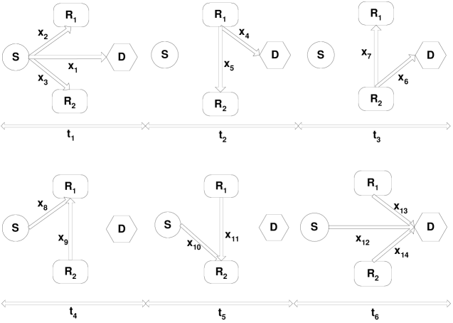
Figure 1: FO protocol for the four-node relay network with $t_{1}+\cdots+t_{6}=1$. The flow optimization is performed over all flows $x_{1},~{}\cdots,~{}x_{14}$, and all time slot lengths $t_{1},~{}\cdots,~{}t_{6}$.

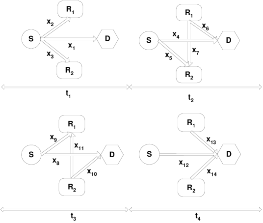
Figure 2: Transmission strategy to obtain a lower bound on the outage probability for the four-node relay network. Here $t_{1}+\cdots+t_{4}=1$, and the optimization is over $x_{1},~{}\cdots,~{}x_{14}$, and $t_{1},~{}\cdots,~{}t_{4}$, with the application of the max-flow-min-cut theorem for the intermediate slots.

For the four-node relay network, there can be 6 possible time slots in the FO protocol as shown in Fig. 1. To derive an upper bound on the achievable rate (and thereby a lower bound on the outage probability), we use max-flow-min-cut type bounds for half-duplex communication. There are four possible time slots as shown in Fig. 2, with the first BC slot and the last MA slot at the destination same as in the FO protocol, but now, the source and a relay may transmit simultaneously to the other relay and the destination during each of the intermediate slots over interference channels. We use the max-flow-min-cut theorem to upper bound the maximum information flow in these two time slots.

For the five-node relay network, there can be 8 possible time slots in the FO protocol - four BC slots for the source and the three relays to transmit information, and four MA slots for the three relays and the destination to receive information respectively. Similar to the four-node relay network case, for the max-flow-min-cut bound, there are $8$ possible time slots with the first BC slot and the last MA slot at the destination being the same as for the FO protocol, and multi-source-multi-destination transmissions during the six intermediate slots.

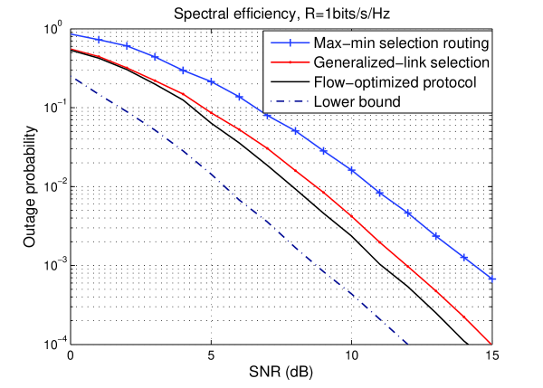
Figure 3: Four-node relay network with uniform average power gains: Outage probabilities for required rate $R=1$bit/s/Hz.

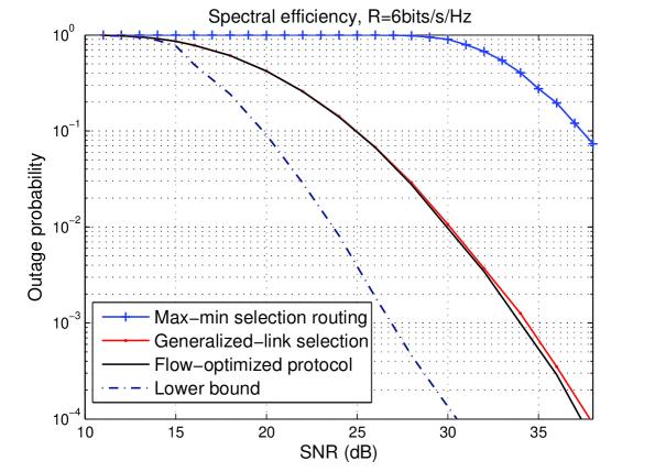
Figure 4: Four-node relay network with uniform average power gains: Outage probabilities for required rate $R=6$bits/s/Hz.

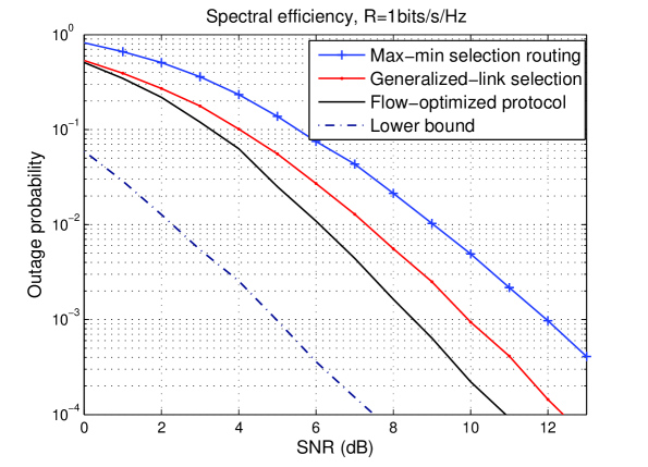
Figure 5: Five-node relay network with uniform average power gains: Outage probabilities for required rate $R=1$bits/s/Hz.

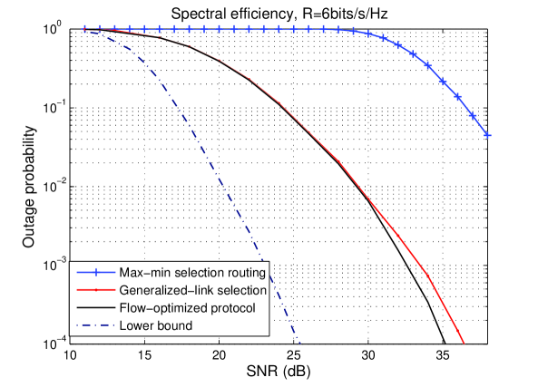
Figure 6: Five-node relay network with uniform average power gains: Outage probabilities for required rate $R=6$bits/s/Hz.

With the above division of time slots, the formalization of the problem is done as in the previous sections, and we use the optimization routine of [20] to obtain the maximum achievable rates and upper bounds for different values of required rates. In Figs. 3 and 4, we plot the outage probabilities of the various schemes with the required rate $R$ at $1$bit/s/Hz and $6$bits/s/Hz respectively, for the four-node relay network. Figs. 5 and 6 present the same for the five-node relay network. When compared to the FO protocol, the GLS protocol suffers a loss of around $1.0$dB, and around $1.5$dB (when $R$ is either $1$bit/s/Hz or $6$bits/s/Hz), at an outage probability of $10^{-4}$, for the four- and five-node relay networks respectively. On the other hand, the performance degradation for the max-min selection method of [11], as compared to the FO protocol or even the GLS protocol, is more than $12$dB at an outage probability of $7.0\times 10^{-2}$, when $R=6$bits/s/Hz for the four-node relay network, and an exactly similar situation can be observed for the five-node relay network. Moreover, for the four-node relay network, the FO protocol is within $2.14$dB (when $R=1$bit/s/Hz) to within $7.05$dB (when $R=6$bits/s/Hz) of the lower bound on the outage probability when the outage probability is $10^{-4}$. For the five-node relay network, the corresponding differences are approximately $3$dB and $9.6$dB respectively.

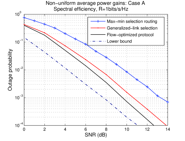
Figure 7: Four-node relay network with non-uniform average power gains. Case A: $\mathbb{E}[Z_{\mathcal{SR}_{1}}]=2.0,~{}\mathbb{E}[Z_{\mathcal{SR}_{2}}]=2.0,~{}\mathbb{E}[Z_{\mathcal{SD}}]=1.0,~{}\mathbb{E}[Z_{\mathcal{R}_{1}\mathcal{R}_{2}}]=1.0,~{}\mathbb{E}[Z_{\mathcal{R}_{1}\mathcal{D}}]=1.5,~{}\mathbb{E}[Z_{\mathcal{R}_{2}\mathcal{D}}]=1.0$. In this case, both the source-relay links are, on average, better than the direct link, and one relay-destination link is, on average, better than the other, resulting in relay $\mathcal{R}_{1}$ being more favorable than relay $\mathcal{R}_{2}$.

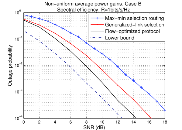
Figure 9: Four-node relay network with non-uniform average power gains. Case B: $\mathbb{E}[Z_{\mathcal{SR}_{1}}]=1.5,~{}\mathbb{E}[Z_{\mathcal{SR}_{2}}]=0.75,~{}\mathbb{E}[Z_{\mathcal{SD}}]=1.0,~{}\mathbb{E}[Z_{\mathcal{R}_{1}\mathcal{R}_{2}}]=3.5,~{}\mathbb{E}[Z_{\mathcal{R}_{1}\mathcal{D}}]=0.2,~{}\mathbb{E}[Z_{\mathcal{R}_{2}\mathcal{D}}]=3.0$. In this case, one source-relay link is, on average, better than the direct link, which, in turn, is better than the other source-relay link. The reverse is true for the relay-destination links, and the inter-relay channel is, on average, very good. This situation promotes inter-relay interactions for the FO protocol, and thereby highlights the sub-optimality of the GLS protocol.

The performances of the different protocols for the four-node relay network with non-uniform average power gains are presented in Figs. 7 and 8, and Figs. 9 and 10 for cases A and B respectively, with the average power gains as stated in the figures. In case A, the source-relay links are, on average, better than the direct link, and one relay node is, on average, a better candidate to forward the information to $\mathcal{D}$. On the other hand, in case B, no one relay has very good source-relay and relay-destination links, whereas the inter-relay link is, on average, very good. This promotes increased inter-relay flows when using the FO protocol, and thereby highlights the limitations of the GLS protocol. The differences between the outage performances of the FO and GLS protocols, at an outage probability of $10^{-4}$, are $1.2$dB or $1.0$dB, and $2.0$dB or $1.3$dB (when $R=1$bits/s/Hz or $R=6$bits/s/Hz), for cases A and B respectively. Thus, the gap between the FO and GLS protocols decreases as the required data rate increases. When the required rate is high, the coding gain offered by a protocol heavily relies on the efficient use of the direct link, and since the usage of the direct link is similar for both the FO and the GLS protocols, the performance gap narrows as the required data rate increases. On the other hand, at the same outage probability, the difference between the outage performance of the FO protocol and the lower bound increases from $1.5$dB to $7$dB, and from $1.9$dB to $6.0$dB as the required rate increases from $1$bit/s/Hz to $6$bits/s/Hz, for cases A and B respectively. Overall, these results demonstrate trends similar to the uniform average power gain case, and confirm the generality of the proposed protocols.

V Conclusions

We proposed a cooperative transmission design for a general multi-node half-duplex wireless relay network. It is based on optimizing information flows, using the basic components of BC and MA, to maximize the transmission rate from the source to the destination, subject to maximum power constraints at individual nodes. We also proposed the simpler GLS protocol, that combines relay selection, and flow optimization for a three-node relay network. These protocols were shown to achieve the optimal DMT for a general relay network. Simulation results for the four- and five-node relay networks for uniform and non-uniform average power gains demonstrate that the performance of the much simpler GLS protocol is close to that of the FO protocol. This suggests that the GLS protocol can be used in systems with low-complexity requirements. We also note that the proposed FO and GLS protocols can be used in wireless networks with topologies more complicated that the wireless relay network considered here. For example, application of similar ideas to a parallel relay network in which there is no direct connection between the source and the destination is considered in [21].

-A Solution to optimization problem (7)

We consider two cases with regard to the link gains: (a) $Z_{\mathcal{SD}}\geq Z_{\mathcal{SR}}$, and (b) $Z_{\mathcal{SD}}<Z_{\mathcal{SR}}$. For both cases, we solve the optimization problem in two stages: first, we fix $t_{1},~{}t_{2}~{}\geq 0$ such that $t_{1}+t_{2}=1$ and find the optimal flows $x_{1},~{}x_{2},~{}x_{3}$ in terms of $t_{1},~{}t_{2}$, and then, find the optimal values for $t_{1},~{}t_{2}$ to maximize the objective function.

$Z_{\mathcal{SD}}\geq Z_{\mathcal{SR}}$

To obtain an analytical solution to the optimization problem and better insight into the nature of the solution to the flow optimization problem, we modify the representation of the BC slot power constraint from that in (7) to the one that is more conventionally used to describe the capacity region of the Gaussian BC channel, as presented in (9). Using the flow constraint in (7), we first solve (9) for fixed $t_{1},~{}t_{2}$.

$$\max(x_{1}+x_{2}+x_{3})~{}~{}\textnormal{over}~{}x_{1},~{}x_{2},~{}x_{3},~{}\alpha,~{}\textnormal{subject to}$$ (9)

$$x_{1},~{}x_{2},~{}x_{3}\geq 0,~{}~{}0\leq\alpha\leq 1,$$

$$x_{1}\leq t_{1}C(Z_{\mathcal{SD}}\alpha S),~{}~{}x_{2}\leq t_{1}C\left(\frac{Z_{\mathcal{SR}}\bar{\alpha}S}{1+Z_{\mathcal{SR}}\alpha S}\right),$$

$$x_{2}\leq t_{2}C(Z_{\mathcal{RD}}S),~{}~{}x_{3}\leq\min\left\{t_{2}C(Z_{\mathcal{SD}}S),~{}t_{2}C(Z_{\mathcal{SD}}S+Z_{\mathcal{RD}}S)-x_{2}\right\}.$$

Here, $\alpha\in[0,1]$ is the fraction of total power spent at the source to transmit $x_{1}$ directly to the destination during the BC slot, and $\bar{\alpha}=1-\alpha$. Although, this modification of the BC slot power constraint apparently makes the optimization problem non-convex owing to the non-convexity in $\alpha$, as we shall see in the sequel, this issue can be handled easily by utilizing the monotonicity of the logarithm function.

Denote the optimal solution by $(x_{1}^{*},x_{2}^{*},x_{3}^{*},\alpha^{*})$ and the corresponding maximum rate by $X(t_{1},t_{2})$. It is clear that $x_{1}^{*}=t_{1}C(Z_{\mathcal{SD}}\alpha^{*}S)$. Suppose that $x_{2}^{*}<t_{1}C\left(\frac{Z_{\mathcal{SR}}\bar{\alpha}^{*}S}{1+Z_{\mathcal{SR}}\alpha^{*}S}\right)$. Since $t_{1}C\left(\frac{Z_{\mathcal{SR}}\bar{\alpha}S}{1+Z_{\mathcal{SR}}\alpha S}\right)$ is a decreasing function of $\alpha$, we can increase $\alpha$ from $\alpha^{*}$ to $\alpha^{0}$ such that $x_{1}^{0}=t_{1}C(Z_{\mathcal{SD}}\alpha^{0}S)>x_{1}^{*}$ and $x_{2}^{*}=t_{1}C\left(\frac{Z_{\mathcal{SR}}\bar{\alpha}^{0}S}{1+Z_{\mathcal{SR}}\alpha^{0}S}\right)$. Thus the objective function becomes $(x_{1}^{0}+x_{2}^{*}+x_{3}^{*})>(x_{1}^{*}+x_{2}^{*}+x_{3}^{*})$ at $\alpha^{0}$. This contradicts the optimality of $(x_{1}^{*},x_{2}^{*},x_{3}^{*},\alpha^{*})$. As a consequence, we have $x_{2}^{*}=t_{1}C\left(\frac{Z_{\mathcal{SR}}\bar{\alpha}^{*}S}{1+Z_{\mathcal{SR}}\alpha^{*}S}\right)\leq t_{2}C(Z_{\mathcal{RD}}S)$. This implies that $\alpha^{*}\geq\max\Bigg{\{}\underbrace{\frac{1}{Z_{\mathcal{SR}}S}\left[\frac{1+Z_{\mathcal{SR}}S}{(1+Z_{\mathcal{RD}}S)^{t_{2}/t_{1}}}-1\right]}_{\alpha_{0}^{a}},0\Bigg{\}},~{}\textnormal{and}~{}\alpha_{a}^{0}\leq 1.$ In essence, this means that the optimal $x_{1}$ and $x_{2}$ should lie on the boundary of the degraded BC capacity region. With this, it is obvious then that $x_{3}=\min\left\{t_{2}C(Z_{\mathcal{SD}}S),~{}t_{2}C(Z_{\mathcal{SD}}S+Z_{\mathcal{RD}}S)-t_{1}C\left(\frac{Z_{\mathcal{SR}}\bar{\alpha}S}{1+Z_{\mathcal{SR}}\alpha S}\right)\right\}$. Therefore the optimization problem of (9) can be re-written as:

$$\displaystyle\max (x_{1}+x_{2}+x_{3})$$ (10)

subject to $$\max\{0,\alpha_{a}^{0}\}\leq\alpha\leq 1,~{}~{}x_{1}=t_{1}C(Z_{\mathcal{SD}}\alpha S),~{}~{}x_{2}=t_{1}C\left(\frac{Z_{\mathcal{SR}}\bar{\alpha}S}{1+Z_{\mathcal{SR}}\alpha S}\right),$$

$$x_{3}=\min\left\{t_{2}C(Z_{\mathcal{SD}}S),~{}t_{2}C(Z_{\mathcal{SD}}S+Z_{\mathcal{RD}}S)-t_{1}C\left(\frac{Z_{\mathcal{SR}}\bar{\alpha}S}{1+Z_{\mathcal{SR}}\alpha S}\right)\right\}.$$

We observe that $x_{3}=t_{2}C(Z_{\mathcal{SD}}S)$ above if and only if

$$\alpha\geq\frac{1}{Z_{\mathcal{SR}}S}\left[\frac{1+Z_{\mathcal{SR}}S}{\left(1+\frac{Z_{\mathcal{RD}}S}{1+Z_{\mathcal{SD}}S}\right)^{t_{2}/t_{1}}}-1\right]\triangleq\alpha_{a}^{1}.$$ (11)

Comparing this to the expression for $\alpha_{a}^{0}$ gives $\alpha_{a}^{0}\leq\alpha_{a}^{1}\leq 1$.

Next we consider two possible sub-cases:

1. $t_{2}C\left(\frac{Z_{\mathcal{RD}}S}{1+Z_{\mathcal{SD}}S}\right)\leq t_{1}C(Z_{\mathcal{SR}}S)$:
   In this case, we have $\bar{\alpha}_{a}^{1}\geq 0$ and $t_{2}\leq\frac{C(Z_{\mathcal{SR}}S)}{C\left(\frac{Z_{\mathcal{RD}}S}{1+Z_{\mathcal{SD}}S}\right)+C(Z_{\mathcal{SR}}S)}~{}\triangleq t_{2\textnormal{max}}$. The maximum rate can be expressed as $X(t_{1},t_{2})=\max\{X_{1}(t_{1},t_{2}),~{}X_{2}(t_{1},t_{2})\}$ where

   $$X_{1}(t_{1},t_{2}) = \max_{\max\{0,\alpha_{a}^{0}\}\leq\alpha\leq\alpha_{a}^{1}}~{}t_{1}C(Z_{\mathcal{SD}}\alpha S)+t_{2}C(Z_{\mathcal{SD}}S+Z_{\mathcal{RD}}S)$$ (12)

   $$= t_{1}C(Z_{\mathcal{SD}}\alpha_{a}^{1}S)+t_{2}C(Z_{\mathcal{SD}}S+Z_{\mathcal{RD}}S)$$

   $$\leq t_{1}\log\left(\frac{(1+Z_{\mathcal{SD}}\alpha_{a}^{1}S)(1+Z_{\mathcal{SR}}S)}{1+Z_{\mathcal{SR}}\alpha_{a}^{1}S}\right)+t_{2}C(Z_{\mathcal{SD}}S)\leq C(Z_{\mathcal{SD}}S)$$

   $$X_{2}(t_{1},t_{2}) = \max_{\alpha_{a}^{1}\leq\alpha\leq 1}~{}t_{1}C(Z_{\mathcal{SD}}\alpha S)+t_{1}C\left(\frac{Z_{\mathcal{SR}}\bar{\alpha}S}{1+Z_{\mathcal{SR}}\alpha S}\right)+t_{2}C(Z_{\mathcal{SD}}S)$$ (13)

   $$= C(Z_{\mathcal{SD}}S)$$

   where the first inequality in (12) holds since (11) is not satisfied, and the second inequality in (12) holds since $\alpha_{a}^{1}\leq 1$ and that the first term in the previous step is monotonically increasing in $\alpha_{a}^{1}$ when $Z_{\mathcal{SD}}\geq Z_{\mathcal{SR}}$. This way, the last observation helps avoid the non-convexity issue mentioned before. Similar arguments hold for $X_{2}(t_{1},t_{2})$ in (13).

2. $t_{2}C\left(\frac{Z_{\mathcal{RD}}S}{1+Z_{\mathcal{SD}}S}\right)>t_{1}C(Z_{\mathcal{SR}}S)$:
   In this case, we have $\alpha_{a}^{1}<0$ and $t_{2}>t_{2\textnormal{max}}$. Thus the maximum rate is given by

   $$X(t_{1},t_{2})=\max_{0\leq\alpha\leq 1}~{}t_{1}C(Z_{\mathcal{SD}}\alpha S)+t_{1}C\left(\frac{Z_{\mathcal{SR}}\bar{\alpha}S}{1+Z_{\mathcal{SR}}\alpha S}\right)+t_{2}C(Z_{\mathcal{SD}}S)=C(Z_{\mathcal{SD}}S).$$ (14)

Hence, (12)–(14) imply that the solution to (9), for any $t_{1},~{}t_{2}$ pair, occurs at $\alpha=1$, and the solution to the original problem of (7), when $Z_{\mathcal{SD}}\geq Z_{\mathcal{SR}}$, is given by $\max_{\{0\leq t_{1},t_{2}~{}:~{}t_{1}+t_{2}=1\}}~{}X(t_{1},t_{2})=C(Z_{\mathcal{SD}}S)$ with any $t_{1},t_{2}$ pair such that $t_{1},t_{2}\geq 0$ and $t_{1}+t_{2}=1$.

$Z_{\mathcal{SD}}<Z_{\mathcal{SR}}$

In this case, the source-relay link is better than the source-destination link. Again, we first fix time slot lengths $t_{1}$ and $t_{2}$ and solve for the optimal values of $x_{1},~{}x_{2},~{}x_{3}$, and $\alpha$, and then maximize the objective function of (7) over all feasible time slot lengths. Following similar arguments as in Case a), the optimization problem of (7) can be re-written as:

$$\max (x_{1}+x_{2}+x_{3})$$ (15)

subject to $$0\leq\bar{\alpha}\leq\min\{1,\bar{\alpha}_{b}^{0}\},~{}~{}x_{1}=t_{1}C\left(\frac{Z_{\mathcal{SD}}\alpha S}{1+Z_{\mathcal{SD}}\bar{\alpha}S}\right),~{}~{}x_{2}=t_{1}C(Z_{\mathcal{SR}}\bar{\alpha}S),$$

$$x_{3}=\min\left\{t_{2}C(Z_{\mathcal{SD}}S),~{}t_{2}C(Z_{\mathcal{SD}}S+Z_{\mathcal{RD}}S)-t_{1}C(Z_{\mathcal{SR}}\bar{\alpha}S)\right\}$$

where $\bar{\alpha}_{b}^{0}=\frac{1}{Z_{\mathcal{SR}}S}\left[(1+Z_{\mathcal{RD}}S)^{t_{2}/t_{1}}-1\right]$ is an upper bound on $\bar{\alpha}$ such that $t_{1}C(Z_{\mathcal{SR}}\bar{\alpha}S)\leq t_{2}C(Z_{\mathcal{RD}}S)$. As before, $x_{3}=t_{2}C(Z_{\mathcal{SD}}S)$ if and only if $\bar{\alpha}\leq\frac{1}{Z_{\mathcal{SR}}S}\left[\left(1+\frac{Z_{\mathcal{RD}}S}{1+Z_{\mathcal{SD}}S}\right)^{t_{2}/t_{1}}-1\right]\triangleq\bar{\alpha}_{b}^{1}$. Also, $0\leq\bar{\alpha}_{b}^{1}\leq\bar{\alpha}_{b}^{0}$. Again, we consider two possible sub-cases:

1. $t_{2}C\left(\frac{Z_{\mathcal{RD}}S}{1+Z_{\mathcal{SD}}S}\right)\leq t_{1}C(Z_{\mathcal{SR}}S)$:
   In this case we have $\bar{\alpha}_{b}^{1}\leq 1$ and $t_{2}\leq\frac{C(Z_{\mathcal{SR}}S)}{C\left(\frac{Z_{\mathcal{RD}}S}{1+Z_{\mathcal{SD}}S}\right)+C(Z_{\mathcal{SR}}S)}~{}\triangleq t_{2\textnormal{max}}$. The maximum rate $X(t_{1},t_{2})$ can be expressed as $X(t_{1},t_{2})=\max\{X_{1}(t_{1},t_{2}),~{}X_{2}(t_{1},t_{2})\}$ where

   $$X_{1}(t_{1},t_{2}) = \max_{0\leq\bar{\alpha}\leq\bar{\alpha}_{b}^{1}}~{}t_{1}C\left(\frac{Z_{\mathcal{SD}}\alpha S}{1+Z_{\mathcal{SD}}\bar{\alpha}S}\right)+t_{1}C(Z_{\mathcal{SR}}\bar{\alpha}S)+t_{2}C(Z_{\mathcal{SD}}S),$$ (16)

   $$X_{2}(t_{1},t_{2}) = \max_{\bar{\alpha}_{b}^{1}\leq\bar{\alpha}\leq\min\{1,\bar{\alpha}_{b}^{0}\}}~{}t_{1}C\left(\frac{Z_{\mathcal{SD}}\alpha S}{1+Z_{\mathcal{SD}}\bar{\alpha}S}\right)+t_{2}C(Z_{\mathcal{SD}}S+Z_{\mathcal{RD}}S),$$ (17)

   and both the maxima in (16) and (17) are attained at $\bar{\alpha}=\bar{\alpha}_{b}^{1}$. Substituting the expression for $\bar{\alpha}_{b}^{1}$ in (16) and (17), we obtain $X_{1}(t_{1},t_{2})=X_{2}(t_{1},t_{2})$ and

   $$X(t_{1},t_{2})=t_{1}\log\left(\frac{1+Z_{\mathcal{SD}}S}{1+\frac{Z_{\mathcal{SD}}}{Z_{\mathcal{SR}}}\left[\left(1+\frac{Z_{\mathcal{RD}}S}{1+Z_{\mathcal{SD}}S}\right)^{t_{2}/t_{1}}-1\right]}\right)+t_{2}C(Z_{\mathcal{SD}}S+Z_{\mathcal{RD}}S).$$ (18)

2. $t_{2}C\left(\frac{Z_{\mathcal{RD}}S}{1+Z_{\mathcal{SD}}S}\right)>t_{1}C(Z_{\mathcal{SR}}S)$:
   In this case we have $\bar{\alpha}_{b}^{1}>1$ and $t_{2}>t_{2\textnormal{max}}$. Thus the maximum rate is given by

   $$X(t_{1},t_{2}) = \max_{0\leq\bar{\alpha}\leq 1}~{}t_{1}C\left(\frac{Z_{\mathcal{SD}}\alpha S}{1+Z_{\mathcal{SD}}\bar{\alpha}S}\right)+t_{1}C(Z_{\mathcal{SR}}\bar{\alpha}S)+t_{2}C(Z_{\mathcal{SD}}S)$$ (19)

   $$= t_{1}C(Z_{\mathcal{SR}}S)+t_{2}C(Z_{\mathcal{SD}}S)$$

   where the maximum occurs at $\bar{\alpha}=1$, as the function to be maximized is monotonically increasing in $\bar{\alpha}$ when $Z_{\mathcal{SR}}>Z_{\mathcal{SD}}$.

Finally, we optimize the above solution to (15) over all possible time slot lengths to obtain the solution to the original problem in (7) when $Z_{\mathcal{SD}}<Z_{\mathcal{SR}}$. Corresponding to Case i. above, when $t_{2}\leq t_{2\textnormal{max}}$, we note that

$$\max_{\{0\leq t_{1},t_{2}:t_{1}+t_{2}=1\}}X(t_{1},t_{2}) \geq X(1-t_{2},t_{2})|_{t_{2}=t_{2\textrm{max}}}$$ (20)

$$= \frac{C(Z_{\mathcal{SR}}S)C(Z_{\mathcal{SD}}S+Z_{\mathcal{RD}}S)}{C(Z_{\mathcal{SR}}S)+C(Z_{\mathcal{RD}}S+Z_{SD}S)-C(Z_{\mathcal{SD}}S)}.$$

On the other hand, corresponding to Case ii., when $t_{2}>t_{2\textnormal{max}}$, from (19), we have

$$\displaystyle\max_{\{0\leq t_{1},t_{2}:~{}t_{1}+t_{2}=1\}}X(t_{1},t_{2}) < (1-t_{2\textrm{max}})C(Z_{\mathcal{SR}}S)+t_{2\textrm{max}}C(Z_{\mathcal{SD}}S)$$ (21)

$$= \frac{C(Z_{\mathcal{SR}}S)C(Z_{\mathcal{SD}}S+Z_{\mathcal{RD}}S)}{C(Z_{\mathcal{SR}}S)+C(Z_{\mathcal{RD}}S+Z_{SD}S)-C(Z_{\mathcal{SD}}S)}$$

where the inequality in (21) is obtained from (19) by using $Z_{\mathcal{SR}}>Z_{\mathcal{SD}}~{}\text{and}~{}t_{2}>t_{2\textrm{max}}$. Hence, from (20) and (21), we conclude that when $Z_{\mathcal{SR}}>Z_{\mathcal{SD}}$, the maximum achievable rate is given by $X(S)=\max_{0\leq t_{2}\leq t_{2\textnormal{max}}}t_{1}\log\left(\frac{1+Z_{\mathcal{SD}}S}{1+\frac{Z_{\mathcal{SD}}}{Z_{\mathcal{SR}}}\left[\left(1+\frac{Z_{\mathcal{RD}}S}{1+Z_{\mathcal{SD}}S}\right)^{t_{2}/t_{1}}-1\right]}\right)+t_{2}C(Z_{\mathcal{SD}}S+Z_{\mathcal{RD}}S)$.

-B Proof of Theorem III.1

In this appendix, we sketch the proof of the theorem. Part 3) of Theorem 4.2 of [14] can be generalized for the $N$-node relay network to prove that, as the block length goes to infinity (during any particular time interval), the average error probability for the FO protocol is upper bounded by its corresponding outage probability. Here, the outage probability denotes the probability that the data rate $R$ cannot be supported by the system when the SNR is $S$, i.e., $P_{\textnormal{out}}(r,S)=\Pr[X(S)<r\log S]$ where $X(S)$ denotes the maximum rate possible for the given channel gain realizations when the SNR is $S$. Thus, from the definition of diversity order (8), we have

$$d(r)\geq\lim_{S\rightarrow\infty}\frac{-\log P_{\textnormal{out}}(r,S)}{\log S}.$$ (22)

Moreover, the above result from [14] can be directly used to prove the same for the GLS protocol. Using this fact, we derive a lower bound to the DMT that can be achieved by the GLS protocol. The sets $I$ and $K$, used in the sequel, are the sets of indices as described in Section III-B. The outage probability for the GLS protocol is given by

$$P_{\textnormal{out}}^{\textnormal{gr}}(r,S)=\Pr\left(\max_{k\in I}X_{k}(S)<r\log S\right)$$ (23)

where $X_{k}(S)$ is the maximum rate achievable by the three-node relay network formed by the source $\mathcal{S}$, the relay $\mathcal{R}_{k}$ and the destination $\mathcal{D}$. We have the following possibilities:

• Case A: $|K|=0$, i.e. the cardinality of the set $K$ is zero. This corresponds to the case when $Z_{\mathcal{SD}}\geq Z_{\mathcal{SR}_{k}}$ for all $k\in I$.

• Case B: $|K|=i$ with $i\in I$.

Note that for Case B there are $N-2\choose i$ possibilities for the set $K$ with cardinality $i$. Since the link gains are assumed to be i.i.d., and the outage probability depends on the distribution of the maximum of $X_{k}(S)$ over all $k\in I$ (or effectively, over all $k\in K$ when $|K|>0$), only the cardinality of $K$ is significant. Let the $N-2\choose i$ possible constructions of the set $K$ be represented by a “generic” set $K_{0}$ with cardinality $i$. Without loss of generality, we describe $K_{0}$ as the set $K$ corresponding to the case when the indices of the relay nodes are ordered according to their source-relay link gains, i.e. $Z_{\mathcal{SR}_{1}}\geq Z_{\mathcal{SR}_{2}}\geq\cdots\geq Z_{\mathcal{SR}_{N-2}}$. Thus, Case B now implies a solitary choice for set $K$, viz. $K_{0}=\{1,2,\cdots,i\}$. Therefore, from (23), we have

$$P_{\textnormal{out}}^{\textnormal{gr}}(r,S) = \Pr\left(C(Z_{\mathcal{SD}}S)<r\log S\middle|~{}|K_{0}|=0\right)\Pr(|K_{0}|=0)$$ (24)

$$+\sum_{i=1}^{N-2}\Pr\left(\max_{k\in K_{0}}X_{k}(S)<r\log S\middle|~{}|K_{0}|=i\right)\Pr(|K_{0}|=i).$$

We observe that using the right-most expression of (20) instead of $X_{k}(S)$, for each $k\in K_{0}$, in (24) gives an upper bound on $P_{\textnormal{out}}^{\textnormal{gr}}(r,S)$. This is utilized in obtaining a lower bound on the diversity order of the GLS protocol. Let $\{S_{n}\}_{n=1}^{\infty}$ be an increasing unbounded sequence of SNRs with $S_{1}>1$. Define the sequence of random variables $\{M_{n}^{k}\}_{n=1}^{\infty}$, $\{B_{n}^{k}\}_{n=1}^{\infty}$ and $\{A_{n}^{k}\}_{n=1}^{\infty}$ with $M_{n}^{k}=\frac{C(Z_{\mathcal{SR}_{k}}S_{n})-C(Z_{\mathcal{SD}}S_{n})}{C(Z_{\mathcal{SD}}S_{n}+Z_{\mathcal{R}_{k}\mathcal{D}}S_{n})}$, $B_{n}^{k}=\frac{C(Z_{\mathcal{SR}_{k}}S_{n})}{\log S_{n}}$, and $A_{n}^{k}=\frac{X_{k}(S_{n})}{\log S_{n}}=\frac{B_{n}^{k}}{1+M_{n}^{k}}$, respectively. Note that for all $k\in K_{0}$, $M_{n}^{k}\rightarrow 0$ a.s. This implies that $(B_{n}^{k}-A_{n}^{k})\rightarrow 0$ a.s. Define $A^{\prime}_{n}=\max_{k\in K_{0}}A_{n}^{k}$ and $B^{\prime}_{n}=\max_{k\in K_{0}}B_{n}^{k}~{}(=B_{n}^{1})$. Then using the above, it can be seen that $(B^{\prime}_{n}-A^{\prime}_{n})\rightarrow 0$ a.s. Further, $\displaystyle\lim_{n\to\infty}\Pr\left(B^{\prime}_{n}<r\middle|~{}|K_{0}|=i\right)$ exists, and therefore the above implies that $\displaystyle\lim_{n\to\infty}\Pr\left(A^{\prime}_{n}<r\middle|~{}|K_{0}|=i\right)=\lim_{n\to\infty}\Pr\left(B^{\prime}_{n}<r\middle|~{}|K_{0}|=i\right)$. Using this in (22) and (24), the diversity order for the GLS protocol, $d^{\textnormal{gr}}(r)$, satisfies

$$\displaystyle d^{\textnormal{gr}}(r) \geq \lim_{S\rightarrow\infty}\frac{-\log P_{\textnormal{out}}^{\textnormal{gr}}(r,S)}{\log S}$$

$$\geq \lim_{n\to\infty}\frac{-1}{\log S_{n}}\log\left[\Pr\left(Z_{\mathcal{SD}}<\frac{S_{n}^{r}-1}{S_{n}}\middle|~{}|K_{0}|=0\right)\Pr(|K_{0}|=0)\right.$$

$$\left.+\sum_{i=1}^{N-2}\Pr\left(Z_{\mathcal{SR}_{1}}<\frac{S_{n}^{r}-1}{S_{n}}\middle|~{}|K_{0}|=i\right)\Pr(|K_{0}|=i)\right]$$

$$= \lim_{n\to\infty}\frac{-1}{\log S_{n}}\log\left[\Pr\left(\max\{Z_{\mathcal{SD}},Z_{\mathcal{SR}_{1}},\cdots,Z_{\mathcal{SR}_{N-2}}\}<\frac{S_{n}^{r}-1}{S_{n}}\middle|~{}|K_{0}|=0\right)\Pr(|K_{0}|=0)\right.$$

$$\left.+\sum_{i=1}^{N-2}\Pr\left(\max\{Z_{\mathcal{SD}},Z_{\mathcal{SR}_{1}},\cdots,Z_{\mathcal{SR}_{N-2}}\}<\frac{S_{n}^{r}-1}{S_{n}}\middle|~{}|K_{0}|=i\right)\Pr(|K_{0}|=i)\right]$$

$$= \lim_{S\to\infty}\frac{-\log\left(\Pr\left(\max\{Z_{\mathcal{SD}},Z_{\mathcal{S}\mathcal{R}_{1}},\cdots,Z_{\mathcal{S}\mathcal{R}_{N-2}}\}<\frac{S^{r}-1}{S}\right)\right)}{\log S}$$

$$= \lim_{S\to\infty}\frac{-\log\left(\left[1-\exp\left(-(S^{r}-1)/S\right)\right]^{N-1}\right)}{\log S}=(N-1)(1-r)$$ (27)

where (-B) is obtained from (-B) by noting that $\max\{Z_{\mathcal{SD}},Z_{\mathcal{SR}_{1}},\cdots,Z_{\mathcal{SR}_{N-2}}\}=Z_{\mathcal{SD}}$ when $|K_{0}|=0$, and $\max\{Z_{\mathcal{SD}},Z_{\mathcal{SR}_{1}},\cdots,Z_{\mathcal{SR}_{N-2}}\}=\max_{k\in K_{0}}Z_{\mathcal{SR}_{k}}=Z_{\mathcal{SR}_{1}}$ when $|K_{0}|>0$, the first equality in (27) is due to the link gains being i.i.d., and the second equality in (27) is obtained by using L’Hospital’s rule.

Next given an $N$-node relay network, consider the multiple access cut that separates the destination from all the other nodes. Clearly, the total flow across this cut gives an upper bound on the maximum rate achievable in the $N$-node relay network. Consequently, a lower bound on the outage probability $P_{\textnormal{out}}^{l}(r,S)$ can be obtained using the maximum sum-rate across this cut:

$$P_{\textrm{out}}^{l}(r,S) \geq \Pr\left[C((Z_{\mathcal{SD}}+Z_{\mathcal{R}_{1}\mathcal{D}}+\cdots+Z_{\mathcal{R}_{N-2}\mathcal{D}})S)<r\log S\right]$$ (28)

$$= \Pr\left[(Z_{\mathcal{SD}}+Z_{\mathcal{R}_{1}\mathcal{D}}+\cdots+Z_{\mathcal{R}_{N-2}\mathcal{D}})<x\right]=\frac{\gamma(N-1,(S^{r}-1)/S)}{\Gamma(N-1)},$$

where $\gamma(a,x)=\int_{0}^{x}t^{a-1}e^{-t}dt$ is the lower incomplete gamma function and $\Gamma(a)=\int_{0}^{\infty}t^{a-1}e^{-t}dt$ is the complete gamma function. The result in part 1) of Theorem 4.2 of [14] can be extended to show that the diversity order of any transmission scheme over the wireless relay network must satisfy

$$\displaystyle d(r) \leq \lim_{S\to\infty}\frac{-\log\left(P_{\textrm{out}}^{l}(r,S)\right)}{\log S}\leq\lim_{S\to\infty}\frac{-\log\left(\frac{\gamma\left(N-1,(S^{r}-1)/S\right)}{(N-2)!}\right)}{\log S}$$ (29)

$$= -\lim_{S\to\infty}\frac{e^{-x}x^{N-2}[S^{-1}-(1-r)S^{r-1}]}{\int_{0}^{x}t^{N-2}e^{-t}dt}=(N-1)(1-r).$$

Finally, from (27) and (29), we see that the GLS protocol, and hence the FO protocol, achieve the optimal DMT of $(N-1)(1-r)$ for all $0<r<1$.

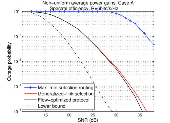
Figure 8: Four-node relay network with non-uniform average power gains. Case A: $\mathbb{E}[Z_{\mathcal{SR}_{1}}]=2.0,~{}\mathbb{E}[Z_{\mathcal{SR}_{2}}]=2.0,~{}\mathbb{E}[Z_{\mathcal{SD}}]=1.0,~{}\mathbb{E}[Z_{\mathcal{R}_{1}\mathcal{R}_{2}}]=1.0,~{}\mathbb{E}[Z_{\mathcal{R}_{1}\mathcal{D}}]=1.5,~{}\mathbb{E}[Z_{\mathcal{R}_{2}\mathcal{D}}]=1.0$. In this case, both the source-relay links are, on average, better than the direct link, and one relay-destination link is, on average, better than the other, resulting in relay $\mathcal{R}_{1}$ being more favorable than relay $\mathcal{R}_{2}$.

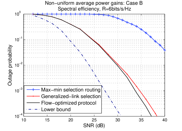
Figure 10: Four-node relay network with non-uniform average power gains. Case B: $\mathbb{E}[Z_{\mathcal{SR}_{1}}]=1.5,~{}\mathbb{E}[Z_{\mathcal{SR}_{2}}]=0.75,~{}\mathbb{E}[Z_{\mathcal{SD}}]=1.0,~{}\mathbb{E}[Z_{\mathcal{R}_{1}\mathcal{R}_{2}}]=3.5,~{}\mathbb{E}[Z_{\mathcal{R}_{1}\mathcal{D}}]=0.2,~{}\mathbb{E}[Z_{\mathcal{R}_{2}\mathcal{D}}]=3.0$. In this case, one source-relay link is, on average, better than the direct link, which, in turn, is better than the other source-relay link. The reverse is true for the relay-destination links, and the inter-relay channel is, on average, very good. This situation promotes inter-relay interactions for the FO protocol, and thereby highlights the sub-optimality of the GLS protocol.

References

• [1] J. N. Laneman, D. N. C. Tse, and G. W. Wornell, “Cooperative Diversity in Wireless Networks: Efficient Protocols and Outage Behavior,” IEEE Transactions on Information Theory, vol. 50, no. 12, pp. 3062–3080, Dec. 2004.
• [2] A. Host-Madsen, and J. Zhang, “Capacity bounds and power allocation for wireless relay channels,” IEEE Transactions on Information Theory, vol. 51, no. 6, pp. 2020–2040, June 2005.
• [3] K. Azarian, H. El Gamal, and P. Schniter, “On the achievable diversity-multiplexing tradeoff in half-duplex cooperative channels,” IEEE Transactions on Information Theory, vol. 51, no. 12, pp. 4152–4172, Dec. 2005.
• [4] A. S. Avestimehr, and D. N. C. Tse, “Outage capacity of the fading relay channel in low SNR regime,” IEEE Transactions on Information Theory, submitted for publication, Feb. 2006.
• [5] D. Gunduz, and E. Erkip, “Opportunistic cooperation by dynamic resource allocation,” IEEE Transactions on Wireless Communications, vol. 6, no. 4, pp. 1446–1454, Apr. 2007.
• [6] L. Ong, and M. Motani, “Optimal Routing for the Gaussian Multiple-Relay Channel with Decode-and-Forward,” in Proc. IEEE SECON 2007, San Diego, U.S.A., Jun. 2007.
• [7] L.-L. Xie, and P. R. Kumar, “A Network Information Theory for Wireless Communication: Scaling Laws and Optimal Operation,” IEEE Transactions on Information Theory, vol. 50, no. 5, pp. 748–767, May 2004.
• [8] G. Kramer, M. Gastpar, and P. Gupta, “Capacity Theorems for Wireless Relay Channels,” IEEE Transactions on Information Theory, vol. 51, no. 9, pp. 3037–3063, Sep. 2005.
• [9] A. Reznik, S. R. Kulkarni, and S. Verdu, “Degraded Gaussian Multirelay Channel: Capacity and Optimal Power Allocation,” IEEE Transactions on Information Theory, vol. 50, no. 12, pp. 3037–3046, Dec. 2004.
• [10] L. Ong, and M. Motani, “The Capacity of the Single Source Multiple Relay Single Destination Mesh Network,” in Proc. IEEE International Symposium on Information Theory (ISIT 2006), Seattle, U.S.A., Jul. 2006.
• [11] A. Bletsas, A. Khisti, D. P. Reed, and A. Lippman, “A Simple Cooperative Diversity Method Based on Network Path Selection,” IEEE Journal on Selected Areas in Communications, vol. 24, No. 3, pp. 659–672, Mar. 2006.
• [12] E. Beres, and R. S. Adve, “On Selection Cooperation in Distributed Networks,” in Proc. Conf. on Information Sciences and Systems (CISS 2006), Mar. 2006.
• [13] J. N. Laneman, and G. W. Wornell, “Distributed space-time-coded protocols for exploiting cooperative diversity in wireless networks,” IEEE Transactions on Information Theory, vol. 49, no. 10, pp. 2415–2425, Oct. 2003.
• [14] T. F. Wong, T. M. Lok, and J. M. Shea, “Flow-optimized Cooperative Transmission for the Relay Channel,” IEEE Transactions on Information Theory, Submitted Dec. 2006. [Online].
Available: http://arxiv.org/PS_cache/cs/pdf/0701/0701019v3.pdf
• [15] L. Zheng, and D. N. C. Tse, “Diversity and multiplexing: A fundamental tradeoff in multiple antenna channels,” IEEE Transactions on Information Theory, vol. 49, no. 5, pp. 1073–1096, May 2003.
• [16] M. Yuksel, and E. Erkip, “Multiple-antenna cooperative wireless systems: A diversity-multiplexing tradeoff perspective,” IEEE Transactions on Information Theory, vol. 53, no. 10, pp. 3371–3393, Oct. 2007.
• [17] T. M. Cover, and J. A. Thomas, Elements of Information Theory, 2nd edition, Wiley, 1991.
• [18] Y. Wu, P. A. Chou, and S.-Y. Kung, “Minimum-Energy Multicast in Mobile Ad Hoc Networks Using Network Coding,” IEEE Transactions on Communications, vol. 53, no. 11, Nov. 2005.
• [19] R. K. Ahuja, T. L. Magnanti, and J. B. Orlin, Network flows: theory, algorithms, and applications, Prentice Hall, 1993.
• [20] C. T. Lawrence, J. L. Zhou, and A. L. Tits, “User’s Guide for CFSQP Version 2.5: A C Code for Solving (Large Scale) Constrained Nonlinear (Minimax) Optimization, Generating Iterates Satisfying All Inequality Constraints,” Technical Report TR-94-16r1, University of Maryland, College Park, 1997.
• [21] W. P. Tam, T. M. Lok, and T. F. Wong, “Flow optimization in parallel relay networks with cooperative relaying,” IEEE Transactions on Wireless Communications, 2008. To appear.
Refer to caption