Modeling the morphogenesis of brine channels in sea ice

Abstract

Brine channels are formed in sea ice under certain constraints and represent a habitat of different microorganisms. The complex system depends on a number of various quantities as salinity, density, pH-value or temperature. Each quantity governs the process of brine channel formation. There exists a strong link between bulk salinity and the presence of brine drainage channels in growing ice with respect to both the horizontal and vertical planes. We develop a suitable phenomenological model for the formation of brine channels both referring to the Ginzburg-Landau-theory of phase transitions as well as to the chemical basis of morphogenesis according to Turing. It is possible to conclude from the critical wavenumber on the size of the structure and the critical parameters. The theoretically deduced transition rates have the same magnitude as the experimental values. The model creates channels of similar size as observed experimentally. An extension of the model towards channels with different sizes is possible. The microstructure of ice determines the albedo feedback and plays therefore an important role for large-scale global circulation models (GCMs).

I Introduction

Formation and decay of complex structures depend on changes in entropy. In the long run structures tend to decay since the entropy of universe leads to a maximum and evolves into a ’dead’ steady state Clausius (1867). On the other hand not only living cells avoid the global thermodynamic equilibrium. A. M. TuringTuring (1952) showed in his paper about the chemical basis of morphogenesis which additional conditions are necessary to develop a pattern or structure. For instance, cells can be formed due to an instability of the homogeneous equilibrium which is triggered by random disturbances. In this sense it should be possible, that the habitat of microorganisms in polar areas, the brine channels in sea ice, can be described through a Turing structure.

The internal surface structure of ice changes dramatically when the ice cools below -23${}^{o}C$ or warms above -5${}^{o}C$ and has a crucial influence on the species composition and distribution within sea ice Light et al. (2003); Krembs et al. (2000). This observation correlates with the change of the coverage of organisms in brine channels between -2${}^{o}C$ and -6${}^{o}C$ Krembs et al. (2000). Golden et al Golden et al. (1998) found a critical brine volume fraction of 5 percent, or a temperature of -5${}^{o}C$ for salinity of 5 parts per thousand where the ice distinguishes between permeable and impermeable behavior concerning energy and nutrient transport. According to Perovich et al Perovich and Gow (1991) the brine volume increases from 2 to 37 ${}^{o}/_{oo}$ and the correlation length increases from 0.14 to 0.22 mm if the temperature rises from -20${}^{o}C$ to -1${}^{o}C$. The permeability varies over more than six orders of magnitude Eicken (2003). Whereas Golden et al Golden et al. (1998) used a percolation model we will demonstrate how the brine channel distribution can be modeled by a reaction-diffusion equation similar to the Ginzburg-Landau treatment of phase transitions. A molecular dynamics simulation shows the change between the hexagonal arranged ice structure and the more disordered liquid water structure Nada et al. (2004).

After a short introduction into the key issue of the structure formation we describe the brine channel structure in sea ice and propose a phenomenological description. For the interpretation of the order parameter we discuss some microscopic properties of water using molecular dynamics simulation in the next chapter II. In chapter III we consider the phase transition and the conditions which allow a structure formation. We verify the model on the basis of measured values in chapter IV and give finally an outlook on further investigations in chapter V.

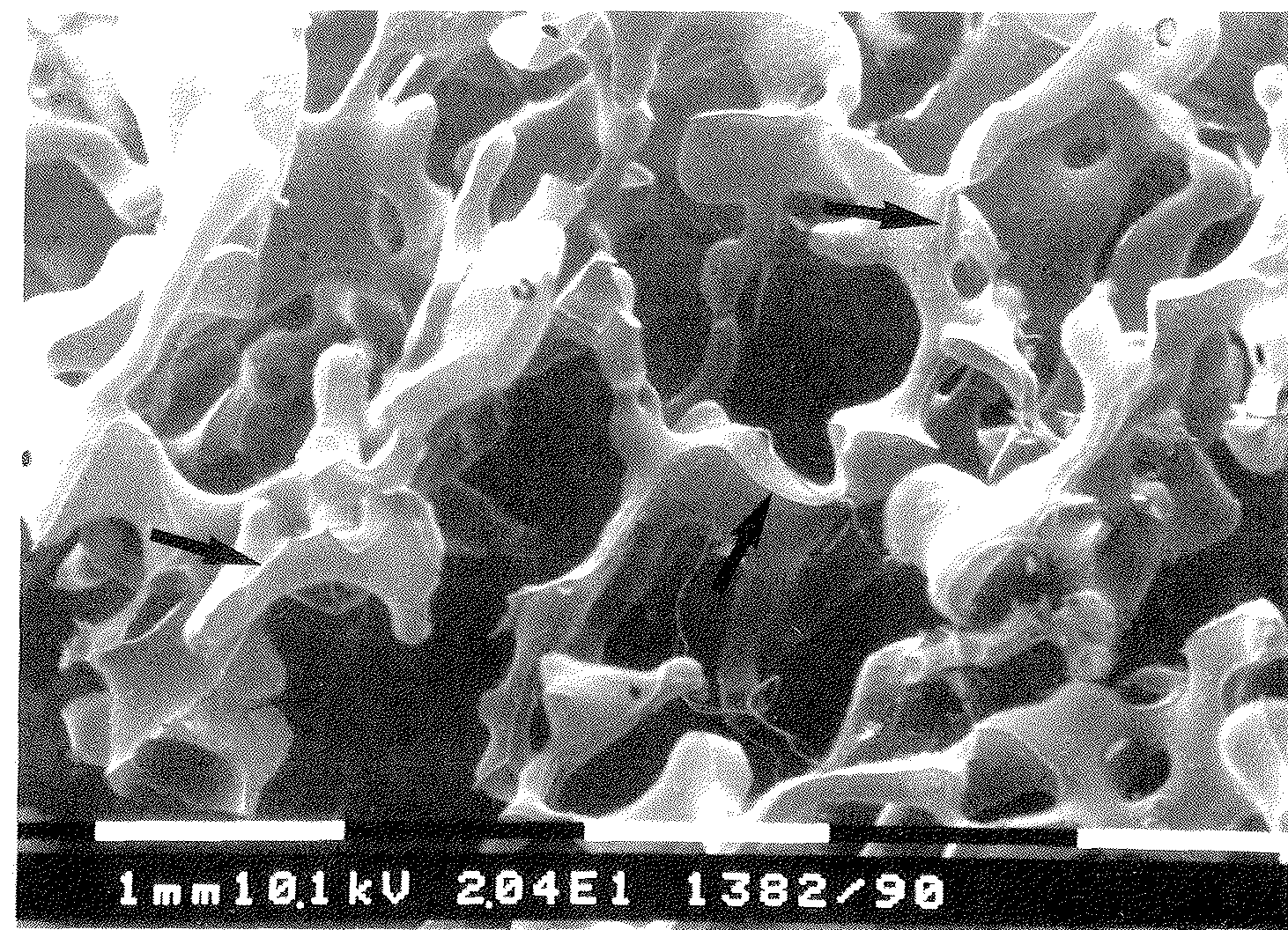
Figure 1: SEM-image of a cast of brine channels Weissenberger (1992).

II Microscopic properties of water

II.1 Formation of brine channels

Various publications report on the life condition for different groups of organisms in the polar areas in brine-filled holes, which arise under certain boundary conditions in sea ice as base- or brine channels (lacuna) Bartsch (1989); Trinks et al. (2005); Weissenberger (1992). They are characterized by the simultaneous existence of different phases, water and ice in a saline environment. Because already marginal temperature variations can disturb this sensitive system, direct measurements of the salinity, temperature, pH-value or ice crystal are morphologically difficult Weissenberger (1992). Weissenberger et al Weissenberger et al. (1992) developed a cast technique in order to examine the channel structure. Freeze-drying eliminates the ice by sublimation, and the hardened casts illustrate the channels as negative pattern. Figure 1 shows a typical granular texture without prevalent orientation.

Sometimes, both columnar and mixed textures occur. Using an imaging system Light et al Light et al. (2003) found brine tubes, brine pockets, bubbles, drained inclusions, transparent areas, and poorly defined inclusions. Air bubbles are much larger than brine pockets. Bubbles possess a mean major axis length of some millimeters and brine pockets are hundred times smaller Perovich and Gow (1996). Cox et al Cox (1983); Cox and Weeks (1983); Cox (1988) presented a quantitative model approach investigating the brine channel volume, salinity profile or heat expansion but without pattern formation. They also described the texture and genetic classification of the sea ice structure experimentally. A crucial factor for the brine channel structure formation is the spatial variability of salinity Cottier et al. (1999).

Different mechanisms are employing the mobility of brine channels which can be used to measure the salinity profile Cottier et al. (1999). Advanced micro-scale photography has been developed to observe in situ the distribution of bottom ice algae Mundy et al. (2007) which allows to determine the variability of the brine channel diameter from bottom to top of the ice. By mesocosm studies the hypothesis was established that the vertical brine stability is the crucial factor for ice algae growth Krembs et al. (2001). Therefore the channel formation during solidification and its dependence on the salinity is of great interest both experimentally and theoretically Worster and Wettlaufer (1997). Experimentally Cottier et al Cottier et al. (1999) presented images, which show the linkages between salinity and brine channel distribution in an ice sample.

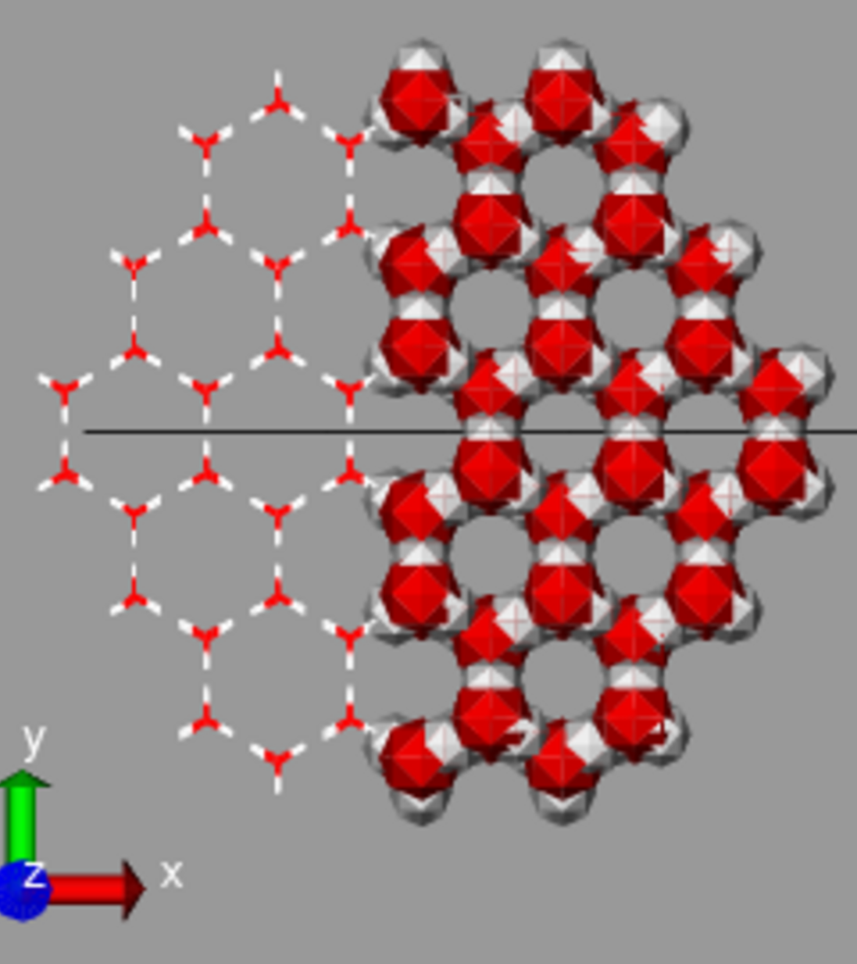
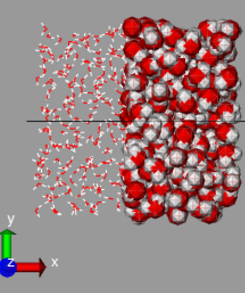
Figure 2: Hexagonal ice (left) and liquid water at 300K (right).

To describe different phases in sea ice dependent on temperature and salinity one possible approach is based on the reaction diffusion system

$$\boldmath\frac{\partial w(x,\mbox{\unboldmath$t$})}{\partial\mbox{\unboldmath$t$}}=f(x,\mbox{\unboldmath$t$})+D\nabla^{2}w(x,\mbox{\unboldmath$t$}),$$ (1)

where $w=\mbox{\unboldmath$\left(\begin{array}[]{c}u\\ v\end{array}\right)$}$ is the vector of reactants, $x=\mbox{\unboldmath$(x,y,z)$}$ the three dimensional space vector, $f$ the nonlinear reaction kinetics and $D=\mbox{\unboldmath$\left(\begin{array}[]{cc}D_{1}&0\\ 0&D_{2}\end{array}\right)$}$ the matrix of diffusitivities, where $D_{1}$ is the diffusion coefficient of water and $D_{2}$ is the diffusion coefficient of salt. For the one- and two-dimensional case we set $y=z=0$ respectively $z=0$. The reaction kinetics described by $f(x,\mbox{\unboldmath$t$})$ can include the theory of phase transitions by Ginzburg-Landau for the order parameters. Referring to this M. Fabrizio Fabrizio (2008) presented an ice-water phase transition. Under certain conditions, spatial patterns evolve in the so-called Turing space. These patterns can reproduce the distribution ranging from sea water with high salinity to sea ice with low salinity. The brine channel system exists below a critical temperature in a thermodynamical non-equilibrium. It is driven via the desalination of ice during the freezing process that leads to a salinity increase in the brine channels. The higher salt concentration in the remaining liquid phase leads to a freezing point depression and triggers the ocean currents.

II.2 Different states of water

Already Wilhelm Conrad Röntgen had described the anomalous properties of water with molecules of the first kind, which he called ice molecules and molecules of the second kind Röntgen (1892) and which represent the liquid aggregate state. Dennison Dennison (1921) determined the ordinary hexagonal ice-I modification from X-ray pattern methodically verified by Bragg Bragg (1922). This so called $E_{h}$-ice is formed by four oxygen atoms which build a tetrahedron as illustrated in figure 2. In $E_{h}$-ice each oxygen atom is tetrahedrically coordinated by four neighbouring oxygen atoms, each accompagnied by a hydrogen bridge. The arrangement is isomorphous to the wurtzite form of zinc sulphide or to the silicon atoms in the tridymite form of silicon dioxide. Bjerrum Bjerrum (1951) and Eisenberg Eisenberg and Kauzmann (2005) have provided a survey about the structure differences between the different polymorphic forms of ice and liquid water.

Molecular dynamics simulations with the TIP3P-model of water using the NAMD-software by the Theoretical and Computational Biophysics Group of the university of Illinois show the change from a regular hexagonal lattice structure to irregular bonds after the melting (figure 2). Nada et al Nada et al. (2004) developed a better six-site potential model of $H_{2}O$ for a crystal growth of ice from water using molecular dynamics and Monte Carlo methods. They computed both the free energy and an order parameter for the description of the water structure. Also Medvedev et al Medvedev and Naberukhin (1987) introduced a ”tetrahedricity measure” $M_{T}$ for the ordering degree of water. It is possible to discriminate between ice- and water molecules via a two-state function ($G=0$ if $M_{T}\geq M^{c}_{T}$ and $G=1$ if $M_{T}<M^{c}_{T}$). This tetrahedricity is computed using the sum

$$M_{T}=\frac{1}{15<l^{2}>}\sum_{i,j}(l_{i}-l_{j})^{2},$$ (2)

where $l_{i}$ are the lengths of the six edges of the tetrahedron formed by the four nearest neighbors of the considered water molecule. For an ideal tetrahedron one has $M_{T}=0$ and the random structure yields $M_{T}=1$. The tetrahedricity can be used in order to define an order parameter according to the Landau - de Gennes model for liquid crystals, which refers to the Clausius-Mosotti-relation. Other simulations such as the percolation models of Stanley et al Stanley (1979); Stanley and Teixeira (1980) use a two-state model, in which a critical correlation length determines the phase transition. A mesoscopic model for the sea ice crystal growth is developed by Kawano and Ohashi Kawano and Ohashi (2009) who used a Voronoi dynamics.

III Reaction - diffusion model

III.1 1+1-dimensional model equations

We consider the reaction diffusion system

$$\frac{\partial u(x,t)}{\partial t} = a_{1}u-cu^{3}+du^{5}+b_{1}v+D_{1}\frac{\partial^{2}u(x,t)}{\partial x^{2}}$$ (3)

$$\frac{\partial v(x,t)}{\partial t} = -a_{2}v-b_{2}u+D_{2}\frac{\partial^{2}v(x,t)}{\partial x^{2}}$$ (4)

in one space dimension. The order parameter according to the Ginzburg-Landau-theory is $u(x,t)$ with $u_{min}\leq u_{c}\leq u_{max}$ and proportional to the tetrahedricity $u\sim M_{T}$. If the variable $u$ is smaller than $u_{c}$ ($u<u_{c}$), the phase changes from water to ice and vice versa. Thus, changes in $u$ reflect temperature variations. The variable $v$ is a measure of the salinity. The coefficient $a_{1}$ depends on the temperature $T$ as $(T-T_{c})/T_{c}$ with the critical temperature $T_{c}$. The salt exchange between ice and water is realized by the gain term $b_{1}v$ and the loss term $-a_{2}v$. The positive terms $a_{1}u$ and $b_{1}v$ are the temperature- and salt-concentration-dependent ”driving forces” of the system.

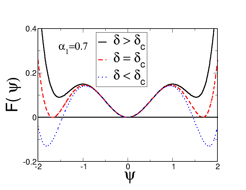
Figure 3: Landau-function (9) versus the dimensionless order parameter (tetrahedricity) for various $\delta$.

In order to realize the $T$-dependent phase transition, one can expand the order parameter in a power series corresponding to Ginzburg and Landau in equation 3. In order to describe properly a temperature-induced phase transition of second order an expression $-cu^{3}$ is necessary. The first-order phase transition is dependent on $du^{5}$. Supercooled or superheated phases can coexist, i.e. an hysteresis behavior is possible. Without the term $du^{5}$ we can also realize a brine channel formation. But this second-order phase transition does not allow us to consider the specific heat as a jump in the order parameter $\psi$ (figures 3 and 4). We write the equations (3) and (4) in dimensionless form (see appendix) by setting $\tau=\sqrt{b_{1}b_{2}}t$, $\xi=\sqrt[4]{{b_{1}b_{2}}/{D^{2}_{1}}}x$, $\psi=\sqrt[4]{{c^{2}}/{b_{1}b_{2}}}u$, $\rho=\sqrt[4]{{b_{1}c^{2}}/{b^{3}_{2}}}v$ and get

$$\frac{\partial\psi(\xi,\tau)}{\partial\tau} = f[\psi,\rho]+\frac{\partial^{2}\psi(\xi,\tau)}{\partial\xi^{2}}$$ (5)

$$\frac{\partial\rho(\xi,\tau)}{\partial\tau} = g[\psi,\rho]+D\frac{\partial^{2}\rho(\xi,\tau)}{\partial\xi^{2}}.$$ (6)

with $\alpha_{1}={a_{1}}/{\sqrt{b_{1}b_{2}}}$, $\delta={d\sqrt{b_{1}b_{2}}}/{c^{2}}$, $\alpha_{2}={a_{2}}/{\sqrt{b_{1}b_{2}}}$ and $D={D_{2}}/{D_{1}}$ as well as the reaction kinetics

$$f[\psi,\rho] = \alpha_{1}\psi-\psi^{3}+\delta\psi^{5}+\rho$$ (7)

$$g[\psi,\rho] = -\alpha_{2}\rho-\psi,$$ (8)

where $\psi$ is the dimensionless order parameter of the water/ice system and $\rho$ the dimensionless salinity. Thus the dynamics only depends on four parameters $\alpha_{1}$, $\alpha_{2}$, $\delta$ and $D$. Without the salinity $\rho$ in equation (3) respectively (5) the above equation system is reduced to a Ginzburg-Landau equation for the first order phase transition.

III.1.1 First Order Phase Transitions

When we neglect the salinity $\rho$, the integration of the kinetic function (7) yields the Landau function for the order parameter $\psi$ of water/ice

$$F = \frac{a_{1}}{2}\psi^{2}-\frac{1}{4}\psi^{4}+\frac{\delta}{6}\psi^{6}$$ (9)

as plotted in figure 3. It possesses three minima

$$\psi_{\rm min}=\left\{0,\pm\sqrt{\frac{1}{2\delta}\left(1+\sqrt{1-4\delta\alpha_{1}}\right)}\right\}.$$ (10)

When several different minima of equal depth exist, then there is a discontinuity in $\psi$ due to Maxwell construction and one has a first-order phase transition Haug (1997). This is the case if

$$\delta=\delta_{c}=\frac{3}{16\alpha_{1c}}$$ (11)

and

$$\psi^{2}_{c}=\frac{3}{4\delta_{c}},$$ (12)

in consequence of

$$F=\psi^{2}\left(\frac{\delta}{6}\left(\psi^{2}-\frac{3}{4\delta}\right)^{2}+\frac{\alpha_{1}}{2}-\frac{3}{2\cdot 16\delta}\right)=0.$$ (13)

Thus the critical parameter $\delta=\delta_{c}$ is determined by the temperature-dependent critical value $\alpha_{1}=\alpha_{1c}$. The jump in figures 3 and 4 is a measure for the latent heat of the phase transition from water to ice. Feistel and Hagen Feistel and Hagen (1998) have deduced theoretically the latent heat of sea ice for various salinities.

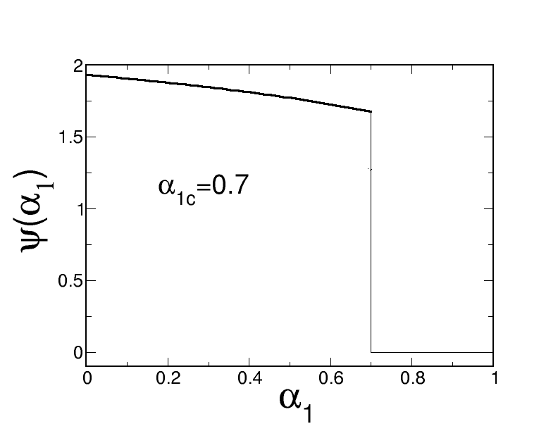
Figure 4: The minimal order parameter $\psi_{\rm min}$ of (10) dependent on $\alpha_{1}$.

III.2 Linear Stability Analysis

First we perform a linear stability analysis by linearizing the equation system (5) and (6) according to $\psi=\psi_{0}+\bar{\psi}$ and $\rho=\rho_{0}+\bar{\rho}$. We obtain the characteristic equation for the fixed points with

$$\left(\begin{array}[]{l}\bar{\psi}\\ \bar{\rho}\end{array}\right)=\left(\begin{array}[]{l}\bar{\psi}_{i}\\ \bar{\rho}_{i}\end{array}\right)exp(\lambda(\kappa)\tau+i\kappa\xi)$$ (18)

as

$$\left(\begin{array}[]{c}\frac{\partial}{\partial{\tau}}\bar{\psi}\\ \frac{\partial}{\partial{\tau}}\bar{\rho}\end{array}\right) = \left(\begin{array}[]{cc}\alpha_{1}-3\psi^{2}_{0}+5\delta\psi^{4}_{0}&1\\ -1&-\alpha_{2}\end{array}\right)\left(\begin{array}[]{c}\bar{\psi}\\ \bar{\rho}\end{array}\right)$$ (25)

$$+ \left(\begin{array}[]{cc}\frac{\partial^{2}}{\partial{\xi^{2}}}&0\\ 0&D\frac{\partial^{2}}{\partial{\xi^{2}}}\end{array}\right)\left(\begin{array}[]{c}\bar{\psi}\\ \bar{\rho}\end{array}\right)$$ (30)

as outlined in appendix.

There are five fixed points for the kinetics (7) and (8) which satisfy $f=0$ and $g=0$. In order to get a stable non-oscillating pattern we need a stable spiral point as fixed point. Moreover the associated eigenvalues have to possess a positive real part for a positive wavenumber, i.e. they have to allow to create unstable modes. Not each fixed point satisfies both conditions. Therefore for the following discussion we choose the steady state, $\psi_{0}=0$ and $\rho_{0}=0$, which corresponds to the observable brine channel structures measured by a casting experiment Mundy et al. (2007); Cottier et al. (1999).

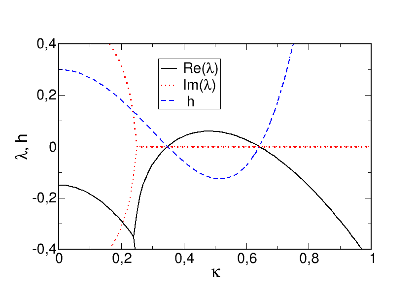
Figure 5: Dispersion of the linear stability (33) versus the dimensionless wave number $\kappa$ for $\alpha_{1}=0.7$, $\alpha_{2}=1$, $D=6$ together with the function $h(\kappa)$ of (32)

Short-time experiments may also record structures that are formed under non-steady conditions. Since those structures are beyond the scope of the present paper, we proceed with the steady state which leads from (30) to

$$\lambda(\kappa)^{2}+[\kappa^{2}(1+D)+\alpha_{2}-\alpha_{1}]\lambda(\kappa)+h(\kappa^{2})=0$$ (31)

with

$$h(\kappa^{2})=D\kappa^{4}+(\alpha_{2}-\alpha_{1}D)\kappa^{2}-\alpha_{1}\alpha_{2}+1$$ (32)

and which is readily solved

$$\lambda(\kappa)_{1,2} = \frac{1}{2}\left(\alpha_{1}-\alpha_{2}-(1+D)\kappa^{2}\right.$$ (33)

$$\left.\pm\sqrt{(\alpha_{1}+\alpha_{2}+(D-1)\kappa^{2})^{2}-4}\right).$$

III.3 Turing space

Let us discuss the equations (31) and (32) concerning the conditions for the occurrance of Turing structures in detail. First we concentrate on the situation $\kappa=0$ where a homogeneous phase is formed. Then the fixed points $\psi=0$ and $\rho=0$ are stable according to the eigenvalues (33) if

$$\lambda_{1,2}(0) = -\frac{\alpha_{2}-\alpha_{1}}{2}\pm\frac{1}{2}\sqrt{(\alpha_{1}-\alpha_{2})^{2}-4(1-\alpha_{1}\alpha_{2})}$$

are negative. Otherwise we would have a globally unstable situation which we rule out. Also homogeneously oscillations don’t describe a brine channel formation. It is easy to see that the solution (LABEL:hom) gives only two negative values if

$${\rm condition}\,{\rm I}:\quad\alpha_{2}>\alpha_{1}\,\,{\rm and}\,\,\alpha_{1}\alpha_{2}<1.$$ (35)

The trajectories of salinity $\rho$ and the order parameter $\psi$ converge to the steady state value zero by damped oscillations. Therefore the structure formation does not follow from the initial condition in time but from the range of the interaction in space.

Next we discuss the spatial inhomogeneous case, $\kappa^{2}>0$, where some spatial fluctuations may be amplified and form macroscopic structures, i.e. the Turing structure. Therefore we search for such modes of (33) which grow in time, i.e. ${\rm Re}\lambda(\kappa)>0$. Time oscillating structures appear if ${\rm Im}\lambda(\kappa)\neq 0$ which can be seen from the solution of (33) to be the case if $\alpha_{1}+\alpha_{2}-2<(1-D)\kappa^{2}<\alpha_{1}+\alpha_{2}+2$. In this region we have

$${\rm Re}\lambda_{\rm osc}(\kappa)={\alpha_{1}-\alpha_{2}-\kappa^{2}(1+D)\over 2}.$$ (36)

Demanding to be positive means $\kappa^{2}(1+D)<\alpha_{1}-\alpha_{2}$. Due to (35) this cannot be fulfilled since the diffusion constant $D$ is positive and $\kappa$ real. Therefore for a time-growing mode we do not have an imaginary part of $\lambda$ in our model. In other words we do not have oscillating and time-growing structures. The restriction for the only allowed region is

$$|(1-D)\kappa^{2}-\alpha_{1}-\alpha_{2}|>2.$$ (37)

In this region we search now for the condition $\lambda>0$. The term before the square in (33) is negative as can be seen from (35). Therefore we can only have positive $\lambda$ if the square of this term is less than the content of the root. This leads to

$$(\alpha_{1}-\kappa^{2})(\alpha_{2}+D\kappa^{2})>1$$ (38)

which restricts the $\kappa$ region to the interval

$$\kappa^{2}\in{1\over 2D}\left(\alpha_{1}D-\alpha_{2}\pm\sqrt{(\alpha_{1}D+\alpha_{2})^{2}-4D}\right).$$ (39)

Due to (35) the term under the square root is samller than the square of the first term in (39) and we get only a meaningful condition from (39) if

$$\alpha_{1}D>\alpha_{2}.$$ (40)

Moreover, the square root must be real, i. e.

$$(\alpha_{1}D+\alpha_{2})^{2}-4D>0,$$ (41)

which leads to

$$D<{(1-\sqrt{1-\alpha_{1}\alpha_{2}})^{2}\over\alpha_{1}^{2}}\quad{\rm or}\quad D>{(1+\sqrt{1-\alpha_{1}\alpha_{2}})^{2}\over\alpha_{1}^{2}}.$$

This has to be in agreement with (40) and discussing the different cases results finally into

$${\rm condition}\,{\rm II}:\qquad D>{(1+\sqrt{1-\alpha_{1}\alpha_{2}})^{2}\over\alpha_{1}^{2}}.$$ (43)

Having determined the ranges of $\alpha_{1}$, $\alpha_{2}$ and $D$ we have to inspect the two conditions on $\kappa$, i.e. (39) and (37). Discussing separately the cases $D\gtrless 1$ one sees that (37) gives no restriction on (39).

Collecting now all conditions for the occurrance of a Turing structure, (43), (35) and (39), we obtain

$${\rm cond.}\,{\rm I}: \quad\alpha_{2}\geq\alpha_{1}\,\,{\rm and}\,\,\alpha_{1}\alpha_{2}\leq 1.$$

$${\rm cond.}\,{\rm II}: \quad D\geq{(1+\sqrt{1-\alpha_{1}\alpha_{2}})^{2}\over\alpha_{1}^{2}}$$

$${\rm cond.}\,{\rm III}: \kappa^{2}\in{1\over 2D}\left(\alpha_{1}D-\alpha_{2}\pm\sqrt{(\alpha_{1}D+\alpha_{2})^{2}-4D}\right).$$

The Turing space as phase diagram is determined by condition I and II and is plotted in figure 6.

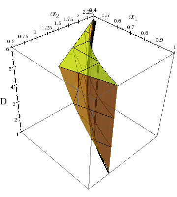
Figure 6: The Turing space as phase diagram where spatial structures can occur. The lower limiting line, $\alpha_{2}=1/\alpha_{1}$, $D=1/\alpha_{1}^{2}$, is plotted as thick line.

One can see that the Turing space starts at the minimal (tricritical point)

$$\alpha_{1t}=\alpha_{2t}=D_{t}=1$$ (45)

which means that we have only a Turing space for sufficient large diffusivity $D\geq 1$. For the Turing space we obtain the possible wave numbers according to condition III as plotted in figure 7.

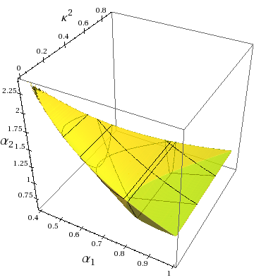
Figure 7: The possible wave lengths $\kappa^{2}$ where spatial structures can occur for $D=6$ in dependence on $\alpha_{1}$ and $\alpha_{2}$.

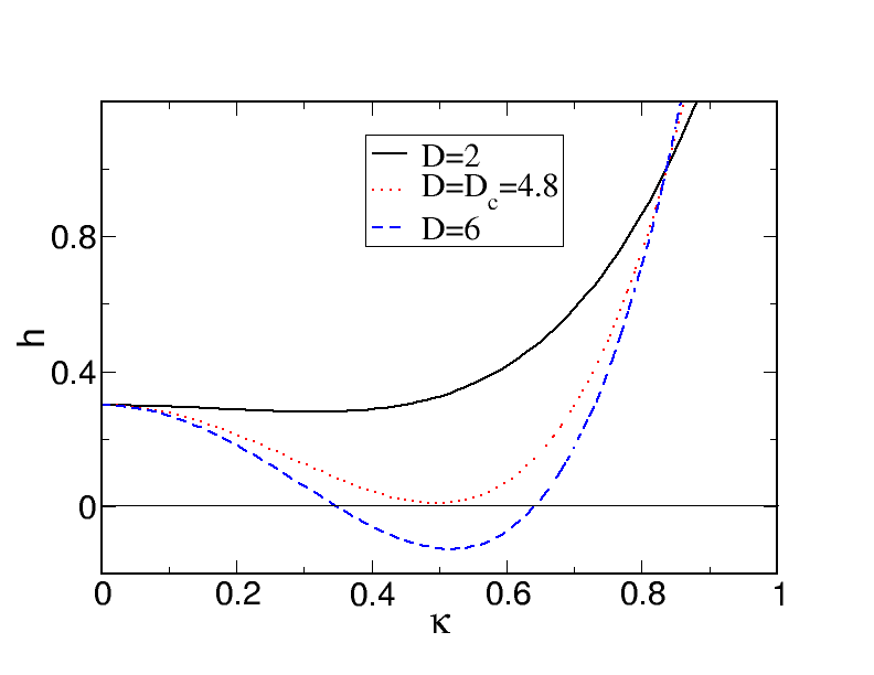
Figure 8: Dispersion $h(\kappa)$ for different $D$, $\alpha_{1}=0.7$ and $\alpha_{2}=1$.

III.4 Critical modes

The critical wavenumber can be found from the largest modes. These are given by the minimum of equation (32) from which we find the wavenumbers

$$\kappa^{2}_{min}=\frac{1}{2D}(Df_{\psi}+g_{\rho})=\frac{1}{2D}(D\alpha_{1}-\alpha_{2})$$ (46)

and the minima

$$h_{min}=f_{\psi}g_{\rho}-g_{\psi}f_{\rho}-\frac{(Df_{\psi}+g_{\rho})^{2}}{4D}=1-\frac{(D\alpha_{1}+\alpha_{2})^{2}}{4D}.$$ (47)

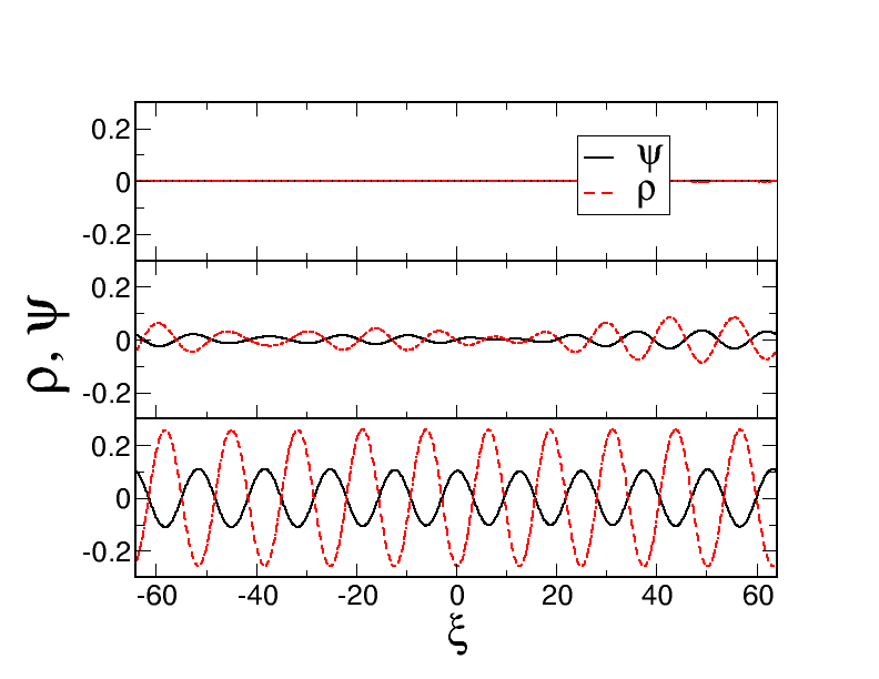
Figure 9: Time evolution of the order parameter $\psi$ and salinity $\rho$ versus spatial coordinates for $\tau=100,170,400$ (from above to below)for $\alpha_{1}=0.7$, $\alpha_{2}=1$, $\delta=\frac{3}{16\alpha_{1}}$, $D=6$ with the initial condition $\rho(\tau=0)=0.5\pm 0.01N(0,1)$ and periodic boundary conditions.

For $\kappa^{2}_{min}>0$ and $h_{min}<0$ we find again the corresponding inequalities (40) and (41). The formation of a spatial Turing structure, a non-oscillating pattern, requires a negative $h_{min}$ for $\kappa^{2}_{min}>0$. In this case there is a range of wavenumbers which are linearly unstable as seen in figure 5. In figure 8 we illustrate the behaviour of $h(\kappa)$ for different diffusion constants. Only those which lead to negative $h$ are forming the Turing structure as discussed in the previous chapter. This critical range can be obtained, if the diffusion coefficient $D$ is greater than the critical diffusion coefficient of condition II, (LABEL:cond) $D_{c}$

$$D_{c}={(1+\sqrt{1-\alpha_{1}\alpha_{2}})^{2}\over\alpha_{1}^{2}},$$ (48)

which we get from $h_{min}=0$ with the critical wavenumber $\kappa_{c}$

$$\kappa^{2}_{c}=\frac{D_{c}f_{\psi}+g_{\rho}}{2D_{c}}=\frac{D_{c}\alpha_{1}-\alpha_{2}}{2D_{c}}.$$ (49)

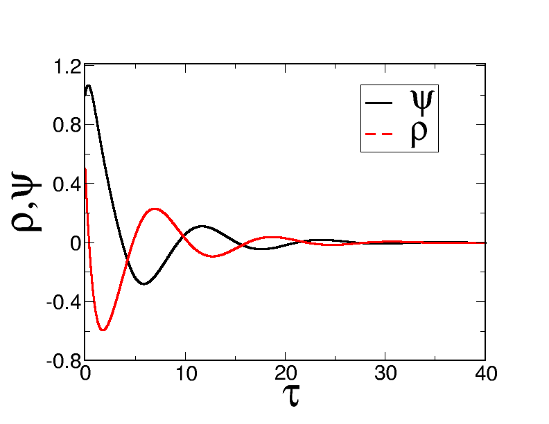
Figure 10: Time evolution of the order parameter $\psi$ and the salinity $\rho$ for $\alpha_{1}=0.7$, $\alpha_{2}=1$, $\delta=\frac{3}{16\alpha_{1}}$ and the initial order parameter $\psi(\tau=0)=1$ and the dimensionsless salinity $\rho(\tau=0)=0.5$.

The size of the structure can be estimated from $\frac{2\pi}{\kappa_{c}}$. The pattern size depends on the both parameters $\alpha_{1}$ and $\alpha_{2}$. The parameters determine the brine channel size and vice versa. With the parameters chosen in fig. 5 we obtain a pattern size of $12.6$. In the next chapter we compare this value with experimental quantities. With a small initial random perturbation we plot snapshots of the time evolution of the order parameter $\psi$ and the salinity $\rho$ in figure 9. The quantities $\psi$ and $\rho$ are opposite to each other; domains with low salinity correspond to domains with ice and domains with high salinity to water domains. We see the formation of a mean mode given by the wave length $\kappa_{c}$.

A positive $h(\kappa=0)$, respectivly a negative $\lambda(\kappa=0)$, for $\kappa=0$ guarantees that $\rho$ and $\psi$ converge to the stable fixed point $\rho_{0}=0,\psi_{0}=0$. Therefore the structure formation does not follow from the initial oscillations in time (fig. 10). In order to obtain a new spatial structure there must exist at least a negative $h$ for $\kappa>0$, respectively a positive eigenvalue $\lambda$, for $\kappa>0$ as was discussed in the last chapter.

III.5 2+1-dimensional model

From the characteristic equation in the spatially two-dimensional case

$$\lambda^{2}+[(\kappa^{2}_{\xi}+\kappa^{2}_{\eta})(1+D)+\alpha_{2}-\alpha_{1}]\lambda+h(\kappa^{2}_{\xi},k^{2}_{\eta})=0$$ (50)

we find the corresponding dispersion relation

$$h(\kappa^{2}_{\xi},\kappa^{2}_{\eta})=D(\kappa^{2}_{\xi}+\kappa^{2}_{\eta})^{2}+(\alpha_{2}-\alpha_{1}D)(\kappa^{2}_{\xi}+\kappa^{2}_{\eta})-\alpha_{1}\alpha_{2}+1$$ (51)

which is illustrated in figure 11.

The Turing space is bounded by the sectional plane $h=0$. The evolution of the order parameter $\psi$ and the salinity $\rho$ is illustrated in figures 12 and 13. Their behavior is inversely proportional and corresponds to the fact, that a high salinity occurs in the water phase and a low salinity in the ice phase. Similiar as in the one-dimensional case we see the dominant formaton of one wavelength. The model kinetics generate brine channels of similar size. In order to obtain a hierarchical net of brine channels of different size, the kinetics in the basic equations can be altered accordingly Murray (1993).

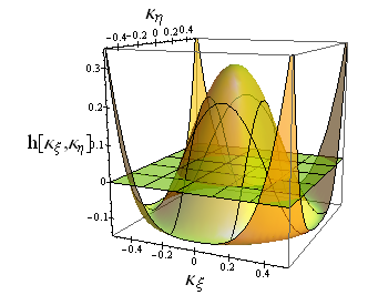
Figure 11: Dispersion of the two-dimensional characteristics (50) and (51) for $\alpha_{1}=0.7$, $\alpha_{2}=1$, $D=6$.

III.6 Note on second and thirth order kinetics

If we replace the kinetics (7) by

$$f[\psi,\rho]=\alpha_{1}\psi-\psi^{3}+\rho$$ (52)

or

$$f[\psi,\rho]=\alpha_{1}\psi-\psi^{2}+\rho$$ (53)

we can carry out the same linear stability analysis for the fixed point $\psi_{0}=0$ and $\rho_{0}=0$. Then we obtain the same characteristic equation as (31) and (32). Therfore we get the same Turing space for the structure formation. Consequently, both kinetics allow us to realize a brine channel formation but the thirth order kinetics describes a second order phase transition only. In this connection it is possible to discuss second order phase transitions with spin models, too.

IV Connection to experimental data

The critical domain size is determined by the equation (49). Due to this relation we can infer other parameters in the model equations (3) and (4). From the relation between the dimensionless wavenumber $\kappa$ and the dimensional wavenumber $k$

$$\kappa^{2}=\frac{\alpha_{1}D-\alpha_{2}}{2D}=\frac{D_{1}}{\sqrt{b_{1}b_{2}}}k^{2}$$ (54)

we get

$$\frac{2\pi}{\kappa_{c}}=12.6=\frac{2\pi}{k_{c}}\frac{\sqrt[4]{b_{1}b_{2}}}{\sqrt{D_{1}}}.$$ (55)

The observed diameters of the brine channels range from $\mu m$ to $mm$ scale Weissenberger (1992). For a size of ${2\pi}/{k_{c}}=10\mu m$ and a diffusion coefficient $D_{1}=10^{-5}{cm^{2}}{s^{-1}}$ for $H_{2}O$-molecules we obtain the product $b_{1}b_{2}=2.5\cdot 10^{6}s^{-2}$ and a transition rate $a_{1}=\sqrt{b_{1}b_{2}}\alpha_{1}=1111s^{-1}$. The rate $a_{1}$ is proportional to reorientations of the molecules per second, ${1}/{\tau_{d}}=10^{5}{s^{-1}}$ (Eisenberg) Eisenberg and Kauzmann (2005) and to the scaled temperature $\frac{T_{c}-T}{T_{c}}$

$$a_{1}\sim\frac{T_{c}-T}{T_{c}}\frac{1}{\tau_{d}},$$ (56)

where $T_{c}$ is the melting point depending on the salinity. The mean salinity in sea ice of $35{g}/{l}$ corresponds to 1 $NaCl$-molecule per 100 $H_{2}O$-molecules, i.e. 1 $Na^{+}$-ion and 1 $Cl^{-}$-ion per 100 $H_{2}O$-molecules in a diluted solution after the dissociation or a ratio of $x=({n_{Na^{+}}+n_{Cl^{-}}})/{n_{H_{2}O}}={1}/{50}$. From this facts we obtain according to Clausius-Clapeyron

$$\Delta T=-\frac{xRT^{2}}{\Delta H}$$ (57)

a freezing point depression from $0^{\circ}C$ to $-2^{\circ}C$, where $\Delta H=6\frac{kJ}{mol}$ is the latent heat of the phase transition from water to ice, $R=8.314\frac{J}{molK}$ is the universal gas constant and $T=273K$. Thus we obtain correctly $T_{c}=271K$. For an environmental temperature of $T=-5^{\circ}C=268K$ according to (56), a transition rate of $\frac{271-268}{271}\cdot 10^{5}s^{-1}=1107s^{-1}$ follows which nearly corresponds to $a_{1}=1111s^{-1}$, which we estimated from the domain size (54).

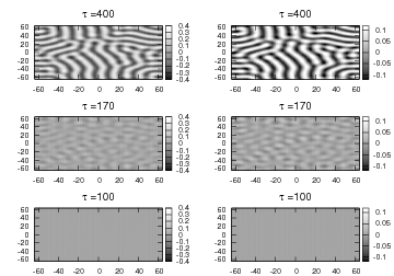
Figure 12: Structure formation for 3 time steps $\tau=100,170,400$ (from top to bottom) for the order parameter $\Psi$ (left) and the salinity $\rho$ (right). The parameters are $a_{1}=0.7$, $a_{2}=1$, $d=\frac{3}{16a_{1}}$, $D=6$ with the initial condition $v(t=0)=0.5\pm 0.01N(0,1)$ and periodic boundary conditions.

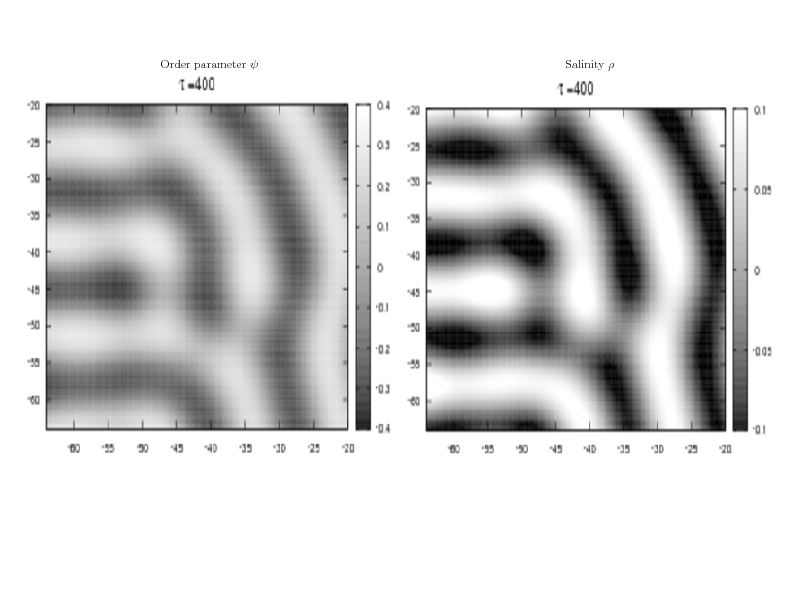
Figure 13: Magnification of a detail of figure 12.

Furthermore we find the transition rate $a_{2}=\sqrt{b_{1}b_{2}}\alpha_{2}=1587s^{-1}$ and the diffusion coefficient $D_{2}=6\times 10^{-5}\frac{cm^{2}}{s}$. Due to the transformation of equation (3) into the dimensionless form (5) there exists a fixed relation (11) because of $c=1$. We obtain for the equation (3) the rate $d_{c}$ with $\alpha_{1}={a_{1}}/{\sqrt{b_{1}b_{2}}}$, $\delta={d\sqrt{b_{1}b_{2}}}/{c^{2}}$ of

$$d_{c}=\frac{3c^{2}}{16a_{1}},$$ (58)

which is proportional to $c^{2}$. A transition rate $c=1000s^{-1}$ yields a critical rate $d_{c}=169s^{-1}$. From the knowledge of the diffusion coefficient $D_{1}$ and the size of brine channels we can deduce the two rates $a_{1}$ and $a_{2}$. Both rates possess the same order of magnitude and are inside the Touring space of structure formation. If the experiments would lead to other parameters $a_{1}$ and $a_{2}$, especially to rather different values, a brine channel could not arise because of the limitation of the Turing space in figure 6 and 7. In other words the model here seems to describe the experimental finding of brine channel formation.

Due to the small difference between the time constants $a_{1}$ and $a_{2}$ we obtain a dynamic interference between the reorientation of the water molecules and the desalinization. Both are evolving on nearly the same time scale. In particular, we cannot simplify the kinetics by separating time scales using the Tichonov theorem Tichonov (1952) in order to reduce our reaction diffusion system (3),(4) but have to consider both dynamics as demonstrated.

V Conclusion

In this paper it has been shown that a reaction diffusion system which connects the basic ideas both of Ginzburg and of Turing can describe the formation of brine channels with realistic parameters. For the chosen parameters patterns of similar size emerged. Eicken Eicken (1991) and Weissenberger Weissenberger (1992) distinguished between six various texture classes of sea ice dependent on the crystal morphology, brine inclusions and the genesis. The different ice crystal growth depends on snow depostion, flooding, turbulent mixing, quiescent growth rate or supercooling. Each condition determines the character of the kinetics. Non-linear heat and salt dissipation for example leads to dendritic growth (snowflakes) whereas one observes in sea ice mostly lamellar or cellular structures rather than complete dendrits Eicken (2003). Hence, the morphology of sea ice is one criterion for the choice of an appropriate kinetics for the genesis of sea ice. Therefore, in order to simulate different structure sizes and textures, we can modify the dispersion relation by varying the parameters $\alpha_{1}$, $\alpha_{2}$ and $D$ or by a modified kinetics Turk (1991). The crucial point is the shape of the dispersion function. If there are multiple different positive unstable regions for the wavenumbers with positive real part of eigenvalues we could expect that differently large channels evolve. For instance Worster et al Worster and Wettlaufer (1997) has presented a general theory for convection with mushy layers. The two different minima of the neutral curve, determined by the linear stability analysis, correspond to two different modes of convection, which affect the kinetics and determines the size distribution of the brine channels. We note that the initial conditions are decisive for the appearance of specific pattern Murray (1993). Hence one should investigate how dislocations or antifreeze proteins influence the formation of the brine channel distribution.

Appendix A Dimensionless Quantities

If we set $\tau=\frac{t}{t_{0}}$, $\xi=\frac{x}{x_{0}}$, $u=C_{1}\psi$ and $v=C_{2}\rho$ we get with $\frac{\partial\psi}{\partial t}=\frac{\partial\tau}{\partial t}\frac{\partial\psi}{\partial\tau}=\frac{1}{t_{0}}\frac{\partial\psi}{\partial\tau}$ and $\frac{\partial\psi}{\partial x}=\frac{\partial\xi}{\partial x}\frac{\partial\psi}{\partial\xi}=\frac{1}{x_{0}}\frac{\partial\psi}{\partial\xi}$

$$\frac{\partial u}{\partial t}=C_{1}\frac{\partial\psi}{\partial t}=\frac{C_{1}}{t_{0}}\frac{\partial\psi}{\partial\tau}$$ (59)

and

$$\frac{\partial u}{\partial x}=C_{1}\frac{\partial\psi}{\partial x}=\frac{C_{1}}{x_{0}}\frac{\partial\psi}{\partial\xi}.$$ (60)

Because of $\frac{\partial^{2}\psi}{\partial\xi^{2}}=\frac{\partial^{2}\psi}{\partial x^{2}}\left(\frac{\partial x}{\partial\xi}\right)^{2}+\frac{\partial\psi}{\partial x}\frac{\partial^{2}x}{\partial\xi^{2}}=x_{0}^{2}\frac{\partial^{2}\psi}{\partial x^{2}}$ we obtain $\frac{\partial^{2}\psi}{\partial x^{2}}=\frac{1}{x^{2}_{0}}\frac{\partial^{2}\psi}{\partial\xi^{2}}$ and consequently

$$\frac{\partial^{2}u}{\partial x^{2}}=C_{1}\frac{\partial^{2}\psi}{\partial x^{2}}=\frac{C_{1}}{x^{2}_{0}}\frac{\partial^{2}\psi}{\partial\xi^{2}}.$$ (61)

Accordingly one has

$$\frac{\partial v}{\partial t} = \frac{C_{2}}{t_{0}}\frac{\partial\rho}{\partial\tau}$$

$$\frac{\partial^{2}v}{\partial x^{2}} = \frac{C_{2}}{x^{2}_{0}}\frac{\partial^{2}\rho}{\partial\xi^{2}}.$$ (62)

From (3) and (4) follow the dimensionless equations

$$\frac{\partial\psi}{\partial\tau} = f[\psi,\rho]+D_{1}\frac{t_{0}}{x^{2}_{0}}\frac{\partial^{2}\psi}{\partial\xi^{2}}$$ (63)

$$\frac{\partial\rho}{\partial\tau} = g[\psi,\rho]+D_{2}\frac{t_{0}}{x^{2}_{0}}\frac{\partial^{2}\rho}{\partial\xi^{2}}$$ (64)

with

$$f[\psi,\rho] = a_{1}t_{0}\psi-ct_{0}C^{2}_{1}\psi^{3}+dt_{0}C^{4}_{1}\psi^{5}+b_{1}t_{0}\frac{C_{2}}{C_{1}}\rho$$

$$g[\psi,\rho] = -a_{2}t_{0}\rho-b_{2}t_{0}\frac{C_{1}}{C_{2}}\psi.$$ (65)

If we choose

$$ct_{0}C^{2}_{1}=1,\qquad b_{1}t_{0}\frac{C_{2}}{C_{1}}=1,$$

$$D_{1}\frac{t_{0}}{x^{2}_{0}}=1,\qquad b_{2}t_{0}\frac{C_{1}}{C_{2}}=1$$ (66)

we obtain $C_{1}=\sqrt[4]{\frac{b_{1}b_{2}}{c^{2}}}$, $C_{2}=\sqrt[4]{\frac{b^{3}_{2}}{b_{1}c^{2}}}$, $t_{0}=\frac{1}{\sqrt{b_{1}b_{2}}}$ and $x_{0}=\sqrt[4]{\frac{D^{2}_{1}}{b_{1}b_{2}}}$.

Appendix B Linear Stability Analysis

Let $\bar{\psi}$ and $\bar{\rho}$ denote small displacements from the equilibrium values $\psi_{0}$ and $\rho_{0}$ and write $\psi=\psi_{0}+\bar{\psi}$ and $\rho=\rho_{0}+\bar{\rho}$. With respect to (5, 6) we obtain

$$\bar{\psi}_{\tau}(\xi,\tau) = \alpha_{1}(\psi_{0}+\bar{\psi})-(\psi_{0}+\bar{\psi})^{3}$$

$$+ \delta(\psi_{0}+\bar{\psi})^{5}+\rho_{0}+\bar{\rho}+\bar{\psi}_{\xi\xi}(\xi,\tau)$$

$$\bar{\rho}_{\tau}(\xi,\tau) = D\bar{\rho}_{\xi\xi}(\xi,\tau)-\alpha_{2}(\rho_{0}+\bar{\rho})-(\psi_{0}+\bar{\psi}).$$ (67)

If we consider only linear terms

$$\bar{\psi}_{\tau}(\xi,\tau) = \cdots+\alpha_{1}\bar{\psi}-3\psi^{2}_{0}\bar{\psi}$$

$$+ 5\delta\psi^{4}_{0}\bar{\psi}+\bar{\rho}+\cdots+\bar{\psi}_{\xi\xi}(\xi,\tau)$$

$$\bar{\rho}_{\tau}(\xi,\tau) = \cdots-\bar{\psi}-\alpha_{2}\bar{\rho}+\cdots+D\bar{\rho}_{\xi\xi}(\xi,\tau)$$ (68)

we get

$$\left(\begin{array}[]{c}\frac{\partial}{\partial{\tau}}\bar{\psi}\\ \frac{\partial}{\partial{\tau}}\bar{\rho}\end{array}\right) = \underbrace{\left(\begin{array}[]{cc}\alpha_{1}-3\psi^{2}_{0}+5\delta\psi^{4}_{0}&1\\ -1&-\alpha_{2}\end{array}\right)}_{\boldmath{J}_{(\psi=\psi_{0},\rho=\rho_{0})}}\left(\begin{array}[]{c}\bar{\psi}\\ \bar{\rho}\end{array}\right)$$ (75)

$$+ \left(\begin{array}[]{cc}\frac{\partial^{2}}{\partial{\xi^{2}}}&0\\ 0&D\frac{\partial^{2}}{\partial{\xi^{2}}}\end{array}\right)\left(\begin{array}[]{c}\bar{\psi}\\ \bar{\rho}\end{array}\right),$$ (80)

where $\boldmath{J}_{(\psi=\psi_{0},\rho=\rho_{0})}$ is the Jacobian

$$\boldmath{J}_{(\psi=\psi_{0},\rho=\rho_{0})} = \left(\begin{array}[]{cc}f_{\psi}&f_{\rho}\\ g_{\psi}&g_{\rho}\end{array}\right)_{(\psi=\psi_{0},\rho=\rho_{0})}$$ (82)

$$= \left(\begin{array}[]{cc}\alpha_{1}-3\psi^{2}_{0}+5\delta\psi^{4}_{0}&1\\ -1&-\alpha_{2}\end{array}\right),$$ (85)

which we can calculate also considering (7, 8).

Using the Fourier ansatz $\bar{\psi}=\psi_{0}exp(\lambda\tau+i\kappa\xi)$ and $\bar{\rho}=\rho_{0}exp(\lambda\tau+i\kappa\xi)$ in (30) we find

$$\left(\begin{array}[]{c}\lambda\bar{\psi}_{i}\\ \lambda\bar{\rho}_{i}\end{array}\right) = \left(\begin{array}[]{cc}\alpha_{1}-3\psi^{2}_{0}+5\delta\psi^{4}_{0}&1\\ -1&-\alpha_{2}\end{array}\right)\left(\begin{array}[]{c}\bar{\psi}_{i}\\ \bar{\rho}_{i}\end{array}\right)$$ (92)

$$+ \left(\begin{array}[]{cc}-\kappa^{2}&0\\ 0&-D\kappa^{2}\end{array}\right)\left(\begin{array}[]{c}\bar{\psi}_{i}\\ \bar{\rho}_{i}\end{array}\right).$$ (97)

With $\psi_{0}=0$ and $\rho_{0}=0$ the eigenvalue equation

$$0=\left[\!\left(\!\begin{array}[]{cc}\kappa^{2}\!-\!\alpha_{1}&-1\\ 1&\alpha_{2}\!+\!D\kappa^{2}\end{array}\right)+\left(\!\begin{array}[]{cc}\lambda&0\\ 0&\lambda\end{array}\right)\right]\!\left(\begin{array}[]{c}\bar{\psi}_{i}\\ \bar{\rho}_{i}\end{array}\right)$$ (104)

follows with the characteristic equation

$$0 = \left|\begin{array}[]{cc}\alpha_{1}-\kappa^{2}-\lambda&1\\ -1&-\alpha_{2}-D\kappa^{2}-\lambda\end{array}\right|$$

$$= \lambda^{2}+[\kappa^{2}(1+D)+\alpha_{2}-\alpha_{1}]\lambda$$

$$+ \underbrace{D\kappa^{4}+(\alpha_{2}-\alpha_{1}D)\kappa^{2}-\alpha_{1}\alpha_{2}+1}_{h(\kappa^{2})}.$$ (108)