Instabilities in non-expanding glasma

Abstract

A homogeneous color magnetic field is known to be unstable for the fluctuations perpendicular to the field in the color space (the Nielsen-Olesen instability). We argue that these unstable modes, exponentially growing, generate an azimuthal magnetic field with the original field being in the $z$-direction, which causes the Nielsen-Olesen instability for another type of fluctuations. The growth rate of the latter unstable mode increases with the momentum $p_{z}$ and can become larger than the former’s growth rate which decreases with increasing $p_{z}$. These features may explain the interplay between the primary and secondary instabilities observed in the real-time simulation of a non-expanding glasma, i.e., stochastically generated anisotropic Yang-Mills fields without expansion.

1 Introduction

Apparent success of hydrodynamic approaches in describing bulk properties of the data in relativistic heavy-ion collisions at BNL-RHIC [1] has stimulated great interest in understanding the mechanism for (possible) short-time thermalization of the system from the initial colliding stage. Preceding studies on this subject [2] include the scenario based on the plasma instability (in particular, the Weibel instability) caused by coupling between hard particles and soft fields [3], the ‘bottom-up’ scenario based on the perturbative scatterings of hard particles [4], and so on. In addition to them, we have recently proposed a novel scenario based on the Nielsen-Olesen (N-O) instability [5] which is characteristic of the configuration of a uniform magnetic field in non-Abelian gauge theories [6, 7]. This scenario applies the earliest time evolution of the system in the heavy ion collision when the separation between hard and soft degrees of freedom is not clear.

In the high-energy limit of collisions, the incident nuclei can be treated as two sheets of classical transverse gluonic fields in the Color Glass Condensate (CGC) framework [8]. This is the QCD effective theory for dense small-$x$ degrees of freedom with treating the large-$x$ components as random colored sources moving on the light cone. With the initial condition given by CGC, it has been shown that longitudinal color electric and magnetic fields are produced just after two infinitesimally thin nuclei pass through each other [9]. Since the correlation length of the fields on the transverse plane is typically $\sim 1/Q_{s}$ with $Q_{s}$ being the saturation scale of colliding nuclei, the emerging configuration after the collision is made of many longitudinal color flux tubes. The produced gluonic system evolving from this unique configuration towards locally thermalized state, providing an equilibrated plasma will be formed, is called glasma [10].

The system of this classical field remains longitudinally boost-invariant during time evolution even though it rapidly expands in the transverse plane and is stretched out in the beam direction. Especially, positive longitudinal pressure is never generated [10, 11], and therefore no thermalization is expected to be achieved. In reality, however, boost-invariance of the system is naturally violated due to finite thickness of the colliding nuclei and quantum fluctuations [12] both of which are in general rapidity dependent. These rapidity-dependent effects may be treated as small fluctuations on top of the boost-invariant classical configurations. The first investigation on the consequences of rapidity-dependent fluctuations was attempted in a numerical simulation of the classical SU(2) Yang-Mills field in an expanding geometry (i.e., in the proper-time and rapidity $\tau$-$\eta$ coodinates) [11] and it was shown that the soft fluctuations indeed grow exponentially, contributing positively to the longitudinal pressure, although the adopted initial fluctuations seemed somewhat too small. This simulation strongly suggests that the boost-invariant system is unstable with respect to the rapidity-dependent soft fluctuations.

Later, analytic studies of the instabilities in the glasma were presented in our works[6, 7] within simplified configurations for the background fields. We revealed that the characteristic features of the rapidity-dependent fluctuations found numerically in Ref. [11] are qualitatively reproduced as the instability of the homogeneous color magnetic field à la Nielsen-Olesen [5]. For example, the maximum longitudinal momentum of the unstable modes contributing to the pressure is shown to increase linearly with the proper-time $\tau$ in accord with the result in Ref. [11].

Recently, another unstable behavior in the classical SU(2) gauge field simulation was reported in Ref. [13] (see also Ref. [14] for SU(3) case). In this simulation, it was observed that (i) there are primary and secondary instabilities, the former of which is identified with the Weibel instability by the authors, and that (ii) the secondary growth rate is larger than the primary growth rate and even increases peculiarly with $p_{z}$. This secondary instability was discussed as nonlinear effects of the primary instability in terms of the re-summed self-energy diagrams in Ref. [13]. In fact, this simulation is quite relevant for physics of the glasma in heavy-ion collisions. The simulation was performed in the Cartesian coordinates without expansion (unlike the glasma), but adopted an extremely anisotropic initial condition in the momentum space which was strongly inspired by the CGC initial condition. More explicitly, the initial configuration was stochastically generated according to the distribution (in the temporal gauge)

$$\left\langle\left|A_{j}^{a}(t=0,{\boldsymbol{p}})\right|^{2}\right\rangle=\frac{C}{(2\pi)^{3/2}\varDelta^{2}\varDelta_{z}}\exp\left\{-\frac{p_{z}^{2}}{2\varDelta_{z}^{2}}-\frac{{\boldsymbol{p}}_{\perp}^{2}}{2\varDelta^{2}}\right\}\,,$$ (1)

with the color index $a=1,2,3$ and the Lorentz index $j=x,y,z$. The normalization parameter $C$ is fixed by the energy density. The variance $\varDelta^{2}$ for the transverse momentum $p_{\perp}=\sqrt{p_{x}^{2}+p_{y}^{2}}$ may be identified with the saturation scale $Q_{s}^{2}$, while $\varDelta_{z}$ for the longitudinal momentum $p_{z}$ is taken as small enough $\varDelta_{z}\ll\varDelta$ to give a $\delta(p_{z})$-like distribution practically. We emphasize here that the initial configuration thus generated will have a nontrivial correlation over the transverse distance $\sim 1/Q_{s}$ while it will be very smooth in the $z$ direction, which is quite similar to the longitudinal flux tubes with rapidity-dependent soft fluctuations in the glasma [11, 7]. Therefore, what was done in Ref. [13] essentially corresponds to the numerical simulation of a non-expanding glasma.

However, there are two points on which we have to be careful in comparing this numerical simulation with the expanding glasma. First, the actual simulation starts with the supplementary condition $E^{a}_{j}=-\dot{A}^{a}_{j}=0$ consistently with the Gauss law. This means that the initial configuration is purely color magnetic in contrast with the expanding glasma which has initially both color electric and magnetic flux tubes. Second, although the magnetic fields generated by the distribution (1) are almost homogeneous in the longitudinal direction, there is no preferred direction of the fields in general. This is in contrast with the expanding glasma whose dominant components are longitudinal. Still, it is certainly possible for some of the flux tubes to have longitudinal polarization in the non-expanding glasma.

In the present paper, we shall discuss a possibility that the primary and secondary instabilities found in Ref. [13] are both induced by the N-O type instability studied in [6, 7]. The ‘primary’ instability occurs in a single flux tube in which there is a strong magnetic field in the longitudinal direction. This analysis is essentially equivalent to the case with the expanding glasma [6, 7]. We will further argue that the ‘primary’ N-O instability will induce a color electric current in the $z$ direction parallel to the original magnetic field, which then generates an azimuthal magnetic field around the current owing to the Ampère law. This new magnetic field can become strong enough to cause the ‘secondary’ N-O instability. The $p_{z}$ dependence of this subsequent instability turns out to be consistent with the findings in Ref. [13].

The present paper is organized as follows. In the next section, we first explain the N-O instability of a homogeneous magnetic field directed to the $z$ direction as an approximation to the magnetic flux tube. We point out qualitative similarities with the primary instability found numerically in Ref. [13]. Then we argue how the color electric current is induced along the $z$ direction by the unstable modes. Stability analysis of the azimuthal color magnetic field generated by the induced current is presented in Section 3. Section 4 is devoted to summary and discussions.

2 The N-O instability and induced current

In this section, we first review the N-O instability of a homogeneous magnetic field in the SU(2) Yang-Mills theory which corresponds to a simplified situation of the magnetic flux tube in the non-expanding glasma. For technical reasons, we formulate everything in the Abelian decomposed representation as in the original presentation by Nielsen and Olesen [5]. We then discuss the consequences of this N-O instability.

2.1 The N-O instability in the Abelian decomposed representation

We study the SU(2) Yang-Mills theory in the temporal gauge $A_{0}^{a}=0$. It has been well known that the configuration of a homogeneous magnetic field in non-Abelian gauge theories exhibits instability with respect to fluctuations perpendicular to the magnetic field in the color space. This is called the Nielsen-Olesen (N-O) instability [5]. This can be most easily understood when we recast the theory in terms of the U(1) “electromagnetic field” $A_{\mu}\equiv A_{\mu}^{3}$ and the “charged vector fields” $\phi_{\mu}\equiv(A_{\mu}^{1}+iA_{\mu}^{2})/\sqrt{2}$  :

$${\mathcal{L}}= -\tfrac{1}{4}F^{a}_{\mu\nu}F^{a\mu\nu}$$

$$= -\tfrac{1}{4}f_{\mu\nu}f^{\mu\nu}-\tfrac{1}{2}|D_{\mu}\phi_{\nu}-D_{\nu}\phi_{\mu}|^{2}+igf^{\mu\nu}\phi_{\mu}^{*}\phi_{\nu}+\tfrac{1}{4}g^{2}(\phi_{\mu}\phi_{\nu}^{*}-\phi_{\nu}\phi_{\mu}^{*})^{2}\;,$$ (2)

where we introduced the U(1) field strength $f_{\mu\nu}=\partial_{\mu}A_{\nu}-\partial_{\nu}A_{\mu}$ and the corresponding covariant derivative $D_{\mu}=\partial_{\mu}+igA_{\mu}$. Notice that we can always gauge transform a homogeneous magnetic field to the 3rd color direction so that it can be represented by the U(1) gauge field. Then, we treat the U(1) gauge field $A_{\mu}$ as a background field, while the charged vector fields $\phi_{\mu}$ as small fluctuations.​ Note that the fluctuations can in principle vary in the $z$ direction, while the background field does not.

We consider a uniform, and time-independent color magnetic field $B>0$ in the $z$ direction which can be generated by $A^{j}=(-\tfrac{1}{2}By,\tfrac{1}{2}Bx,0)$. The $\phi$-dependent part of the energy density is now written as (in the temporal gauge $A_{0}=\phi_{0}=0$)

$$\mathcal{E}_{\phi}= |\dot{\phi}^{i}|^{2}+\tfrac{1}{2}|D^{i}\phi^{j}-D^{j}\phi^{i}|^{2}-igf^{ij}\phi^{i*}\phi^{j}-\tfrac{1}{4}g^{2}(\phi^{i*}\phi^{j}-\phi^{i}\phi^{j*})^{2}$$

$$= |\dot{\phi}^{+}|^{2}+|\dot{\phi}^{-}|^{2}+|{\boldsymbol{D}}\phi^{+}|^{2}+|{\boldsymbol{D}}\phi^{-}|^{2}+2gB|\phi^{+}|^{2}-2gB|\phi^{-}|^{2}$$

$$+|\dot{\phi}^{z}|^{2}+|{\boldsymbol{D}}\phi^{z}|^{2}-\tfrac{1}{4}g^{2}(\phi^{i*}\phi^{j}-\phi^{i}\phi^{j*})^{2}$$ (3)

with ${\boldsymbol{D}}={\boldsymbol{\nabla}}-ig{\boldsymbol{A}}$ and $\phi^{\pm}=\tfrac{1}{\sqrt{2}}(\phi^{x}\pm i\phi^{y})$ in the ‘spin’ basis. In the second line we neglected the surface term and exploited, for simplicity,​ the condition $D_{i}\phi^{i}=0$, which is consistent with the non-Abelian part of the Gauss law of the SU(2) gauge theory

$$D_{i}\dot{\phi}^{i}+ig\dot{A}^{i}\phi^{i}=0\;,$$ (4)

since the background field is now time-independent $\dot{A}^{i}=0$. Furthermore, the physical solution $\phi^{i}$ to the Yang-Mills equation must satisfy the Abelian part of the Gauss law

$$\partial_{i}\dot{A}^{i}-ig(\phi^{i}\dot{\phi}^{i*}-\phi^{i*}\dot{\phi}^{i})=0\;,$$ (5)

which simplifies to $\phi^{i}\dot{\phi}^{i*}-\phi^{i*}\dot{\phi}^{i}=0$ when $\dot{A}^{i}=0$. We stress here that the SU(2) gauge field theory inevitably involves the non-minimal spin coupling $[D^{\mu},D^{\nu}]\phi_{\mu}^{*}\phi_{\nu}\sim igf^{\mu\nu}\phi_{\mu}^{*}\phi_{\nu}$ between $A_{\mu}$ and $\phi_{\mu}$ in addition to the minimal ones $-\frac{1}{2}|D_{\mu}\phi_{\nu}|^{2}$ when decomposed with respect to the U(1) subgroup. While this non-minimal coupling entails mixing of $\phi^{x}$ and $\phi^{y}$, it can be diagonalized by the introduction of $\phi^{\pm}$ as seen in the second line of Eq. (3). Thus, in a magnetic field, the charged vector fields $\phi^{\pm}$ acquire the “Zeeman” energy $\pm 2gB$ through this non-minimal coupling. This is the origin of the N-O instability as we will see below.

Within the linear approximation with respect to the fluctuations $\phi^{\pm}$, we find the equation of motion for $\phi^{\pm}$

$$\left(\partial_{t}^{2}-{\boldsymbol{D}}^{2}\pm 2gB\right)\phi^{\pm}=0\,,$$ (6)

with ${\boldsymbol{D}}^{2}=\nabla^{2}-\frac{1}{4}g^{2}B^{2}(x^{2}+y^{2})+igB(y\partial_{x}-x\partial_{y})$. We can solve it in a similar way as in the quantum Hall effects and obtain the eigenfrequencies with the longitudinal momentum $p_{z}$ as

$$\omega^{2}=p_{z}^{2}+gB(2n+|m|-m+1)\pm 2gB\,,$$ (7)

where $n=0,1,2,\cdots$ is the principal quantum number of a two-dimensional harmonic oscillator and $m=0,\pm 1,\pm 2,\cdots$ is the eigenvalue of two-dimensional angular momentum $L_{z}=i(x\partial_{y}-y\partial_{x})$. The factor in the brackets can be written as $2n+|m|-m+1\equiv 2N+1$ with $N=0,1,2,\cdots$ specifying the Landau levels. Each Landau level is degenerate in $m\geq 0$, but we simply set $m=0$ since it is irrelevant to the discussion below. Note that the frequency for the lowest Landau level $N=n=0$ of $\phi^{-}$ (and $\phi^{-*}\equiv(\phi^{x*}+i\phi^{y*})/\sqrt{2}$, too) allows pure imaginary values for small $p_{z}$ satisfying $p_{z}^{2}<gB$ due to the non-minimal coupling, which indicates that the fluctuation grows exponentially $\phi^{-}\propto{\rm e}^{\gamma t}$ with the growth rate $\gamma=|{\rm Im}\ \omega|$. This is the instability Nielsen and Olesen pointed out some time ago [5]. In this ideal case of the uniform magnetic field, $\gamma$ is given by

$$\gamma(p_{z})=|{\rm Im}\ \omega|=\sqrt{gB-p_{z}^{2}}\,.$$ (8)

Clearly, the fastest instability occurs at $p_{z}=0$ with the maximum growth rate $\gamma_{\rm max}=\sqrt{gB}$. Here, we should notice that existence of the unstable mode at $p_{z}=0$ is a unique feature of the N-O instability in clear contrast with the Weibel instability, which is familiar in the plasma-instability scenario. In fact, the Weibel instability takes place when charged particles with an anisotropic distribution move in a soft inhomogeneous magnetic field with the ‘minimal’ particle-field coupling [3]. Inhomogeneity of the soft magnetic field is indispensable for an anisotropic distribution of the charged particles to show filamentation along this very inhomogeneity inducing a current, which then creates a magnetic field additively to the original field. Thus, the Weibel instability cannot occur in the homogeneous limit $p_{z}\to 0$.

The simplest situation discussed above still has some relevance to the inhomogeneous background magnetic field on the transverse ($xy$) plane as far as the typical modulating distance $R_{\perp}$ and the typical strength $B$ of the magnetic field satisfy the condition $R_{\perp}\mathrel{\hbox to0.0pt{\raise 2.20013pt\hbox{$>$}\hss}{\lower 2.20013pt\hbox{$\sim$}}}1/\sqrt{gB}$. This is because the unstable mode in a uniform magnetic field $B$ is localized in a transverse region of a size $1/\sqrt{gB}$ as is evident from the explicit form of the solution (in the $p_{z}$ representation):

$$\widetilde{\phi}^{-}_{\rm unstable}(t,x_{\perp},p_{z})\propto{\rm exp}\left\{\gamma(p_{z})t-\frac{1}{4}gBx_{\perp}^{2}\right\}\,.$$ (9)

As discussed in Introduction, the expanding glasma in heavy-ion collisions is initially an assembly of many longitudinal color flux tubes whose transverse correlation length is typically given by $Q_{s}^{-1}$. Since the color magnetic field inside the flux tube is roughly estimated as $B\sim{\mathcal{O}}(Q_{s}^{2}/g)$, the transverse size of the unstable mode of the N-O instability is also given by $1/\sqrt{gB}\sim Q_{s}^{-1}$. Therefore, in this case, the condition $R_{\perp}\mathrel{\hbox to0.0pt{\raise 2.20013pt\hbox{$>$}\hss}{\lower 2.20013pt\hbox{$\sim$}}}1/\sqrt{gB}$ is merginally satisfied, indicating the relevance of the N-O instability in the expanding glasma [7]. The same should be true for the glasma without expansion if the similar estimate for the color magnetic field strength holds. In fact, as mentioned in Introduction, the numerical simulation in Ref. [13] was performed choosing the initial condition similar to that of the expanding glasma. Therefore, it seems plausible that the primary instability found in Ref. [13] is due to the Nielsen-Olesen instability. The observed growth rate of the primary instability indeed shows very similar $p_{z}$ dependence as Eq. (8), especially it remains nonzero at $p_{z}=0$.

A more rigorous analysis would require to solve Eq. (6) numerically with the magnetic field $B$ generated randomly on the transverse plane via Eq. (1). Then a negative eigenvalue $\omega^{2}$ of a solution indicates an unstable mode. Although existence of an unstable mode in such a generic background is not obvious at all, it is quite reasonable that the (largest) growth rate of the unstable mode, if exists, will be smaller than the estimate $\sqrt{g|B_{\rm max}|}$ where $|B_{\rm max}|$ is the maximum value of the inhomogeneous magnetic field. This can be intuitively understood if one recognizes that the magnetic field $B$ corresponds to a ‘potential’ in Eq. (6): a positive (negative) $B$ works as an attractive (repulsive) potential well for the fluctuation field $\phi^{-}$ and the unstable modes are regarded as ‘bound states’ trapped in this potential. If one considers a bound state (for small $p_{z}$) in a single potential well with a certain depth, the ‘binding energy’ becomes smaller in general as the potential gets more localized. In other words, if we define an effective magnetic field $B_{\rm eff}$ with the (largest) negative eigenvalue of $\omega^{2}$ as $\omega^{2}\equiv-gB_{\rm eff}$, then we have $B_{\rm eff}<|B_{\rm max}|$. Furthermore, we may expect that the qualitative dependence of the growth rate on the momentum $p_{z}$ will be unchanged from the uniform field case. This is because the momentum $p_{z}$ always enters the eigenfrequency $\omega^{2}$ in the same way as in Eq. (7), as far as there is no $p_{z}$ dependence in the background magnetic field. After all, the $p_{z}$ dependence of the growth rate $\gamma$ in an inhomogeneous magnetic field will be represented[6] with the effective magnetic field as

$$\gamma(p_{z})\simeq\sqrt{gB_{\rm eff}-p_{z}^{2}}\,,$$ (10)

and the maximum momentum for the instability will be given by $p_{z}^{\rm max}=\sqrt{gB_{\rm eff}}$.

2.2 Induced current and the azimuthal magnetic field

The exponential growth of the unstable modes cannot last forever. When the amplitude of the unstable fluctuation $\phi^{-}$ becomes sizeable, we need to include the effects of nonlinear interaction between fluctuations which were ignored in the stability analysis of the homogeneous magnetic field. In fact, the charged matter fields have a double-well potential similar to the Higgs field (see Eq. (3)), and thus it is quite reasonable that the instability will cease when the fluctuation becomes as large as $\phi^{-}\sim\sqrt{8B/g}$, corresponding to the bottom of the potential. However, this is not the end of the story. In this subsection, we discuss the consequences of this enhanced fluctuations.

We claim that the enhanced fluctuations will induce a large color electric current in the longitudinal direction, which then generates an azimuthal magnetic field according to the Ampère law. Here we define the ‘induced U(1) current’ for the U(1) gauge field in the Lagrangian: $J^{\mu}=\delta{\mathcal{L}}/\delta A_{\mu}$. Its $z$-component is given by

$$J^{z}=\sum_{\alpha=\pm}ig\left\{\phi^{\alpha*}D^{z}\phi^{\alpha}-(D^{z}\phi^{\alpha})^{\ast}\phi^{\alpha}\right\}\,.$$ (11)

Being made of the charged fluctuations $\phi^{\pm}$, this current flows in the presence of a color electric field in the $z$ direction. This also implies that the current will be enhanced if the fluctuations grow exponentially. Recall that the unstable mode can have longitudinal momentum $p^{z}\mathrel{\hbox to0.0pt{\raise 2.20013pt\hbox{$<$}\hss}{\lower 2.20013pt\hbox{$\sim$}}}\sqrt{gB}$, and thus one may count the order of the covariant derivative $D^{z}$ in the current as $D^{z}\sim{\cal O}(\sqrt{gB})$. If the fluctuation grows up to the same order as its saturation value $\phi^{-}\sim{\cal O}(\sqrt{B/g})$, magnitude of the induced current can be roughly evaluated as

$$J^{z}\sim{\mathcal{O}}(g\cdot\sqrt{gB}\cdot{B}/{g})={\mathcal{O}}((gB)^{3/2}/g)\sim{\mathcal{O}}(Q_{s}^{3}/g)\,,$$ (12)

where we have used an estimate $\sqrt{gB}\sim Q_{s}$. Note that this current can be parametrically very large.

The induced current in the $z$ direction creates azimuthal magnetic field $B^{\theta}$ around it according to the Ampère law: ${\boldsymbol{J}}={\rm rot}\,{\boldsymbol{B}}$ (in the present case $J^{z}=\frac{1}{r}\partial_{r}(rB^{\theta})$ if one considers only the $z$ component), where the azimuthal magnetic field $B^{\theta}$ can be as strong as the initial magnetic field:

$$B^{\theta}={\mathcal{O}}(Q_{s}^{2}/g)\,.$$ (13)

For a localized current $J^{z}>0$ in a finite region of the size $1/Q_{s}$ on the transverse plane, the Ampère law implies that the azimuthal magnetic field becomes maximum at the brim of the current with the strength estimated as in Eq. (13), and it decays only slowly as $B^{\theta}(r)\propto 1/r$ outside the region of the nonzero current. In the next section, we argue that thus generated azimuthal magnetic field is again unstable against the Nielsen-Olesen mechanism.

Admittedly, our discussion on the induced current (12) presented here is only order-of-magnitude estimate. More accurate evaluation of the magnitude will require an analysis of nontrivial time evolution of the background field (in particular, the longitudinal color electric field $E^{z}=-\partial_{t}A^{z}$) due to coupling between the background field and the enhanced fluctuation, which certainly goes beyond the linear analysis. Also more inputs from non-perturbative numerical simulations will be very useful. One may be able to argue some possible mechanisms to generate the induced current, but at present it is quite difficult to provide a solid picture for that. We thus leave the definite analysis as an open problem for future study.

3 Effects of azimuthal magnetic field $B^{\theta}$

We have seen in the previous section that the homogeneous color magnetic field directed to the 3rd color and to the $z$ spatial direction undergoes the N-O instability, and that the enhanced fluctuations induce a current in the $z$ direction, which in turn generates an azimuthal magnetic field $B^{\theta}$. In this section, we shall investigate the consequences of the presence of this newly created magnetic field. As already discussed, the induced current starts to flow according to the generation of longitudinal color electric field $E^{z}$. Thus, the azimuthal magnetic field will become stronger with increasing time. In this section, however, we treat $B^{\theta}$ as time-independent since we are interested in instabilities which will take place in a very short period. Still, it would be very helpful to investigate two different situations: (i) when $B^{\theta}$ is weak enough and can be treated as perturbation to the original magnetic field $B^{z}$, and (ii) when there is a strong $B^{\theta}$. In the latter case, we will ignore the effects of $B^{z}$ which will be screened by the ‘primary’ N-O instability.

Stability analysis in the presence of the azimuthal magnetic field is conveniently formulated in the cylindrical coordinates $(r,\theta,z)$ with $x=r\cos\theta$ and $y=r\sin\theta$. For simplicity, we consider a constant color magnetic field $\mbox{\boldmath$B$}=(B^{r}=0,B^{\theta},B^{z})$ which is generated by the gauge field : $(A^{r},A^{\theta},A^{z})=(0,\tfrac{1}{2}rB^{z},-rB^{\theta})$. We again treat the charged vector field $\phi_{\mu}$ as fluctuation and perform the linear approximation in the equations of motion for $\phi^{i}$. Then one finds three coupled equations among $\phi^{r}$, $\phi^{\theta}$ and $\phi^{z}$ (in the temporal gauge $\phi^{0}=0$):

$$\partial_{t}^{2}\phi^{r}-{\boldsymbol{D}}^{2}\phi^{r}+\frac{2}{r}D_{\theta}\phi^{\theta}+\frac{1}{r^{2}}\phi^{r}+2igB^{z}\phi^{\theta}-2igB^{\theta}\phi^{z}=0\,,$$ (14)

$$\partial_{t}^{2}\phi^{\theta}-{\boldsymbol{D}}^{2}\phi^{\theta}-\frac{2}{r}D_{\theta}\phi^{r}+\frac{1}{r^{2}}\phi^{\theta}-2igB^{z}\phi^{r}=0\,,$$ (15)

$$\partial_{t}^{2}\phi^{z}-{\boldsymbol{D}}^{2}\phi^{z}+2igB^{\theta}\phi^{r}=0\,,$$ (16)

where ${\boldsymbol{D}}^{2}=D_{z}^{2}+\partial_{r}^{2}+\frac{1}{r}\partial_{r}+D_{\theta}^{2}$ and $D_{\theta}=\frac{1}{r}\partial_{\theta}-igA^{\theta}$. Note that it is the azimuthal field $B^{\theta}$ which couples the field $\phi^{z}$ to the transverse field $\phi^{r}$. In fact, when the azimuthal magnetic field is absent $B^{\theta}=0$, Eqs. (14) and (15) reduce to Eq. (6) for $\phi^{\pm}=(\phi^{r}\pm i\phi^{\theta})e^{\pm i\theta}/\sqrt{2}$.

3.1 $B^{\theta}$ as perturbation to $B^{z}$

Before we present the stability analysis of the azimuthal magnetic field, let us examine how the results obtained in the previous section will change in the presence of small perturbation of $B^{\theta}$. First of all, we rewrite Eqs. (14) and (15) in terms of $\widetilde{\phi}^{\pm}$ and $\widetilde{\phi}^{z}$ (in the $p_{z}$ representation) as

$$\left\{\partial_{t}^{2}+\left({p_{z}}-gB^{\theta}r\right)^{2}-\frac{1}{r}\partial_{r}(r\partial_{r})-D_{\theta}^{2}\pm 2gB^{z}\right\}\widetilde{\phi}^{\pm}= 2igB^{\theta}\widetilde{\phi}^{z}\,.$$ (17)

Compared with Eq. (6), one indeed verifies that the azimuthal field $B^{\theta}$ adds the coupling with $\phi^{z}$ and shifts the longitudinal momentum $p_{z}$ in our gauge. Consider the unstable fluctuation $\widetilde{\phi}^{-}$ and ignore the stable one $\widetilde{\phi}^{z}$. When the azimuthal magnetic field is much weaker than the longitudinal magnetic field $B^{\theta}\ll B^{z}$, we take only the term linearly dependent on $B^{\theta}$:

$$\left\{\left(\partial_{t}^{2}-{\boldsymbol{D}}_{(0)}^{2}-2gB^{z}\right)-2gB^{\theta}rp_{z}\right\}\widetilde{\phi}^{-}=0\,,$$ (18)

where we have introduced ${\boldsymbol{D}}_{(0)}^{2}=\nabla_{\perp}^{2}-p_{z}^{2}-\frac{1}{4}g^{2}(B^{z})^{2}r^{2}$ for zero angular momentum states, with the subscript (0) indicating that $B^{\theta}=0$. Taking the last term in the curly brackets as perturbation, we find that the lowest eigenfrequency (squared) is modified in the leading order of perturbation as

$$\omega^{2}_{n=0}=p_{z}^{2}-gB^{z}-2gB^{\theta}\langle r\rangle\,p_{z}\,,$$ (19)

where the average $\langle r\rangle$ is taken over the unperturbed solution given by Eq. (9), i.e., $\langle r\rangle=\int_{0}^{\infty}rdr\widetilde{\phi}^{-*}r\widetilde{\phi}^{-}/\int_{0}^{\infty}rdr\widetilde{\phi}^{-*}\widetilde{\phi}^{-}\propto 1/\sqrt{gB^{z}}$. This eigenvalue $\omega^{2}_{n=0}$ can become negative for the momentum $p_{z}$ such that

$$-\sqrt{gB^{z}}+gB^{\theta}\langle r\rangle<p_{z}<\sqrt{gB^{z}}+gB^{\theta}\langle r\rangle\,,$$ (20)

yielding instability with the growth rate

$$\gamma(p_{z})\simeq\sqrt{gB^{z}+2gB^{\theta}\langle r\rangle p_{z}-p_{z}^{2}}\,,$$ (21)

where we have ignored the contribution quadratic in $B^{\theta}$. The maximum momentum for the instability is given by $p_{z}^{\rm max}\simeq\sqrt{gB^{z}}+gB^{\theta}\langle r\rangle=\sqrt{gB^{z}}(1+cB^{\theta}/B^{z})$ with $c=\sqrt{\pi/2}$, and the unstable region in the $p_{z}$ space slightly shifts to larger $p_{z}$. On the other hand, the maximum value of the growth rate $\gamma=|{\rm Im}\,\omega|$ is still given by $\sqrt{gB^{z}}$ in the leading order perturbation. A schematic picture of the growth rate as a function of $p_{z}$ is shown in Fig. 1.

Let us summarize here our understanding of the ‘primary’ N-O instability. The simplest picture with a constant magnetic field $B^{z}$ should be modified at two points: (i) inhomogeneity of the magnetic field on the transverse plane, and (ii) the presence of $B^{\theta}$. The first point works to diminish the growth rate, and the second one works to shift the instability region in the $p_{z}$ space slightly to the right, to form an oval shape. These two effects seem to be qualitatively in agreement with the primary instability obtained in the numerical simulation [13].

Figure 1: A schematic picture of the growth rate $\gamma=|\text{Im}\,\omega|$ of the ‘primary’ N-O instability. Solid (dashed) line is the growth rate with (without) a weak azimuthal magnetic field.

3.2 Instability of the azimuthal magnetic field $B^{\theta}$

Let us finally present the stability analysis of the azimuthal magnetic field $B^{\theta}$. In order to understand the effects of $B^{\theta}$, we consider the simplest case with $B^{z}=0$ which is however reasonable because the original magnetic field will be weakened by the enhanced fluctuations. Then, Eqs. (14) and (16) are nearly diagonalized by combining the fields as $\varphi^{\pm}=(\phi^{z}\pm i\phi^{r})/\sqrt{2}$ :

$$\partial_{t}^{2}\varphi^{+}-{\boldsymbol{D}}^{2}\varphi^{+}+\frac{1}{2r^{2}}\left(\varphi^{+}-\varphi^{-}\right)+2gB^{\theta}\varphi^{+}=0\,,$$ (22)

$$\partial_{t}^{2}\varphi^{-}-{\boldsymbol{D}}^{2}\varphi^{-}-\frac{1}{2r^{2}}\left(\varphi^{+}-\varphi^{-}\right)-2gB^{\theta}\varphi^{-}=0\,,$$ (23)

where we have again restricted ourselves to the states with $\partial_{\theta}=0$ and the operator ${\boldsymbol{D}}^{2}$ is now given by ${\boldsymbol{D}}^{2}=D_{z}^{2}+\partial_{r}^{2}+\frac{1}{r}\partial_{r}$. When $B^{\theta}>0$, the structure of these equations suggests that instabilities will occur for $\varphi^{-}$ due to the negative potential term $-2gB^{\theta}$. Therefore, we solve the equation for $\varphi^{-}$ assuming that $\varphi^{+}$ is small compared to $\varphi^{-}$. By setting $\varphi^{+}=0$, one finds an equation for $\widetilde{\varphi}^{-}\propto e^{-i\omega t+ip_{z}z}$ :

$$\Bigl{\{}-\frac{1}{r}\frac{d}{dr}r\frac{d}{dr}+\left(p_{z}-gB^{\theta}r\right)^{2}+\frac{1}{2r^{2}}-2gB^{\theta}\Bigr{\}}\,\widetilde{\varphi}^{-}(r)=\omega^{2}\,\widetilde{\varphi}^{-}(r)\,.$$ (24)

This is the equation to be solved. Note that the equation has only one parameter $\rho_{0}\equiv p_{z}/\sqrt{gB^{\theta}}$, which becomes evident if one rewrites it in terms of a dimensionless variable $\rho=\sqrt{gB^{\theta}}r$:

$$\Bigl{\{}-\frac{1}{\rho}\frac{d}{d\rho}\rho\frac{d}{d\rho}+\left(\rho-\rho_{0}\right)^{2}+\frac{1}{2\rho^{2}}-2\Bigr{\}}\,\widetilde{\varphi}^{-}=\epsilon\,\widetilde{\varphi}^{-}\,,$$ (25)

where $\epsilon=\omega^{2}/gB^{\theta}$ is the normalized eigenfrequency. If one further rescales the fluctuation field as $\widetilde{\varphi}^{-}(\rho)\equiv\,\rho^{-1/2}\,\psi(\rho)$, then one obtains a simple one dimensional Schrödinger equation:

$$\left(-\frac{d^{2}}{d\rho^{2}}+V(\rho)\right)\psi(\rho)=\epsilon\,\psi(\rho)\,,\quad V(\rho)\equiv\frac{1}{4\rho^{2}}+(\rho-\rho_{0})^{2}-2\,.$$ (26)

The explicit form of the potential $V(\rho)$ is shown in Fig. 2 for three different values of $\rho_{0}$. The potential is singular at $\rho=0$ because of the ‘centrifugal’ potential acting on the $m=0$ state, inherent to the vector field, and takes a negative value at the minimum which moves outwards with increasing $\rho_{0}$.

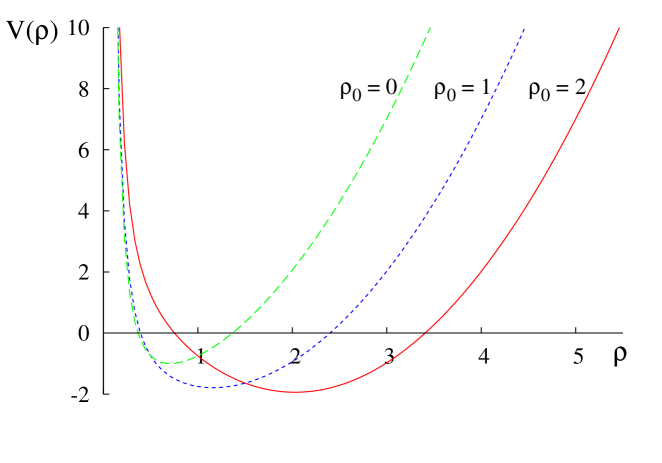
Figure 2: Potential $V(\rho)$ for three different values of $\rho_{0}$. The potential minimum moves outwards with increasing $\rho_{0}$.

Let us first consider the case with large $\rho_{0}$ (high $p_{z}$). In this case, the centrifugal potential is negligible around the minimum, and thus the equation reduces to that of a harmonic oscillator located at $\rho=\rho_{0}$. The eigenvalue of the harmonic oscillator then gives approximate solutions to the equation for large $\rho_{0}$, namely, $\epsilon_{n}=(2n+1)-2\,$ with $n=0,1,2,\cdots$. Clearly, the ground state has the negative eigenvalue, $\epsilon_{n=0}=-1$ because of the last term “$-2$” whose origin can be traced back to the non-minimal coupling between the magnetic field and the fluctuation in Eq. (24). The negative eigenvalue $\omega^{2}=-gB^{\theta}$ implies the existence of an unstable mode with the growth rate $\gamma_{\theta}^{\infty}=\sqrt{gB^{\theta}}$. Notice that this result has no $p_{z}$ dependence. This is because the longitudinal momentum $p_{z}$ (or $\rho_{0}$) only determines the position of the harmonic oscillator, but does not enter the spectrum. The first correction to this harmonic oscillator approximation comes from the centrifugal potential, and yields the following $p_{z}$ dependent growth rate ($\rho_{0}=p_{z}/\sqrt{gB^{\theta}}$)

$$\gamma_{\theta}(p_{z})\simeq\sqrt{gB^{\theta}}\sqrt{1-\frac{1}{4\rho_{0}^{2}}}\,.$$ (27)

Therefore, it is an increasing function of $p_{z}$, and approaches the harmonic oscillator result $\gamma_{\theta}^{\infty}=\sqrt{gB^{\theta}}$ in the limit $p_{z}\to\infty$. It should be emphasized that this instability occurs at larger $p_{z}$, in contrast to the case of the N-O instability in a homogeneous $B^{z}$.

Next we consider the case with small $\rho_{0}$ (low $p_{z}$). Notice that the growth rate (27) becomes smaller for smaller $\rho_{0}$. In fact, the equation (26) in the limit $\rho_{0}=0$ can be exactly solved by the confluent hypergeometric function with the eigenvalues $\epsilon_{n}=4n+\sqrt{2}$ for $n=0,1,2,\cdots$[15]. All the eigenvalues are positive, and therefore the system is stable when $p_{z}=0$. This implies that there is a minimum value of $p_{z}$ for the instability.

Summarizing these analytic studies, we find that the instability indeed occurs at relatively large $p_{z}$ with the growth rate given as an increasing function of $p_{z}$, while there will be no unstable modes for small values of $p_{z}$. We can directly check that these expectations are indeed the case by solving numerically Eq. (24). The result is shown in Fig. 3 where the (normalized) growth rate $\gamma_{\theta}/\sqrt{gB^{\theta}}$ is plotted as a function of $p_{z}/\sqrt{gB^{\theta}}$. In accordance with the analytic result (shown as the dashed line in Fig. 3), the instability appears only for larger $p_{z}/\sqrt{gB^{\theta}}\geq 0.755$ and the growth rate indeed increases towards the asymptotic value $\gamma_{\theta}^{\infty}=\sqrt{gB^{\theta}}$ with increasing $p_{z}$. This is the notable feature and consistent with the behavior observed for the secondary instability in Ref. [13]. We also draw the wavefunctions $\psi(\rho)$ in Fig. 4 corresponding to the three different potentials shown in Fig. 2. The wavefunctions are well localized around $\rho=\rho_{0}$ and vanishes at $\rho=0$. The same is true for the original fluctuation field $\widetilde{\varphi}^{-}(\rho)=\rho^{-1/2}\psi(\rho)$. Therefore, we expect that, as far as $p_{z}$ is not too large, our analysis with the homogeneous azimuthal magnetic field is not a bad approximation to more realistic cases with $B^{\theta}(\rho=0)=0$ and $B^{\theta}(\rho\gg 1)\sim 1/\rho$.

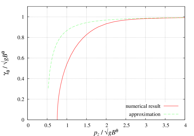
Figure 3: Growth rate $\gamma_{\theta}(p_{z})=|{\rm Im}\,\omega|$ of the unstable mode in the azimuthal magnetic field $B^{\theta}$. Solid line: numerical result from Eq. (26), dashed line: approximate result, Eq. (27) valid at large $p_{z}$.

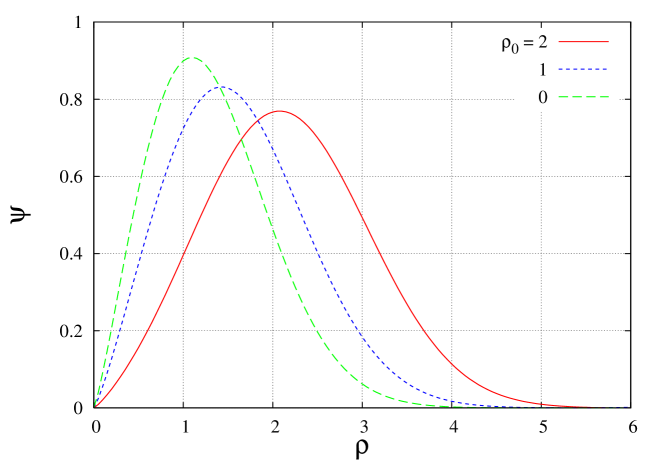
Figure 4: Rescaled wavefunction $\psi(\rho)$ as a solution to Eq. (26) for three different potentials shown in Fig. 2. The case of $\rho_{0}=0$ is stable, while the other two are unstable.

4 Summary and discussions

We have studied instabilities in the configuration with the azimuthal magnetic field in the SU(2) Yang-Mills theory, as a possible mechanism for the secondary instability observed in the classical stochastic simulation [13].

The instability of an expanding glasma numerically found in Ref. [11] was previously interpreted as the Nielsen-Olesen instability of the longitudinally uniform color magnetic fields produced in between two sheets of the Color Glass Condensates [6, 7]. Although the simulation in Ref. [13] was performed in the Cartesian coordinates, the adopted initial condition was extremely anisotropic in the momentum space, which is inherent to the collision dynamics, and we consider the primary instability observed there has the same origin as the one in Ref. [11].

We have argued that the charged fields grow up due to the N-O instability and are accelerated in the evolving background gauge field, inducing a current possibly along the $z$ axis. This current will generates the azimuthal magnetic field, whose strength $B^{\theta}$ can grow exponentially in time at early stage. The induction of the current and its strength is the most speculative part of our discussion beyond the linear analysis.

We have shown that, once the azimuthal magnetic field becomes strong enough, this configuration is subsequently accompanied by the N-O instability with respect to another type of fluctuation. We have analyzed this new instability in some detail, and shown that the growth rate increases with the momentum $p_{z}$. This is in contrast with the growth rate of the primary N-O instability which decreases with increasing $p_{z}$ and vanishes at some value of $p_{z}$. The effects of the azimuthal magnetic fields on the primary instability are to enlarge the value of the momentum at which the growth rates vanish. These findings coincide quite well with the results in the simulation in Ref. [13].

The N-O instability scenario for the secondary instability is generic to the Yang-Mills systems with an anisotropic configuration, and therefore it should, in principle, apply to the case of expanding glasmas, too. In the numerical simulation in Ref. [11], however, the secondary instability was not clearly observed. This might be because they started the simulation with extremely small fluctuations. On the other hand, in Ref. [13], the initial amplitudes of the fluctuations were not assumed small (actually, this scale non-separation was one of their motivations for taking the numerical approach). Nevertheless, it is intriguing to note that, reexamining the pressure evolution started with relatively larger fluctuations shown in Ref. [11], one can barely see a subtle kink, which may hint the secondary instability. In fact, the increase of the longitudinal pressure at late time can be attributed to the generation of the transverse magnetic fields, and this is consistent with our scenario. Another indication of the secondary instability is an abrupt increase of the maximum longitudinal momentum $\nu_{\rm max}(\tau)$ of the unstable modes. Since the slope $C$ of the linear growth $\nu_{\rm max}(\tau)=C\tau$ at earlier time is found to be proportional to the growth rate [6, 7], it is plausible to relate the sudden increase of $\nu_{\rm max}(\tau)$ to the emergence of another instability with a larger growth rate. Other possible scenarios are previously discussed in Ref. [11]. It is thus a pressing subject to analyze specifically the course of the expanding glasma evolution from the viewpoint of the N-O instability.

Our analysis seems to indicate that in the glasma evolution the sequential appearance of instabilities play a key role to make the system more random and turbulent towards thermalization. Of course, our discussion is based on the simple stability analysis and speculation on the induced current. Especially more solid discussions on the generation of the azimuthal magnetic field and the back-reaction from the well-developed unstable mode will require careful analyses on the system configuration and evolution which will be accessible in numerical simulations. Moreover, simulations in Ref. [13] should involve the Weibel instability mechanism also in principle, although they were formulated in terms of the classical fields. Hence, coexistence of the Weibel and the N-O instabilities in the evolving system is worthwhile to be studied. In this context, more joint efforts in analytic and numerical approaches are to be accomplished in this field.

Acknowledgements
This work was completed during the workshop on “Non-equilibrium quantum field theories and dynamic critical phenomena” at the Yukawa Institute of Theoretical Physics in March 2009. H.F. and K.I. thank useful and extensive discussions with the participants, in particular with Jürgen Berges. A.I. is grateful to members of KEK theory group and of Komaba nuclear theory group for kind hospitality. This work is partly supported by Grants-in-Aid (18740169 (K.I.) and 19540273 (H.F.)) of MEXT.

References

- [1] For example, U. W. Heinz and P. F. Kolb, “Two RHIC puzzles: Early thermalization and the HBT problem,” arXiv: hep-ph/0204061.
- [2] For a brief review, see K. Itakura, Prog. Theor. Phys. Suppl. 168 (2007) 295.
- [3] For a recent review, see S. Mrowczynski, PoS C POD2006 (2006) 042 [arXiv:hep-ph/0611067].
- [4] R. Baier, A. H. Mueller, D. Schiff and D. T. Son, Phys. Lett. B 502 (2001) 51 [arXiv:hep-ph/0009237].
- [5] N. K. Nielsen and P. Olesen, Nucl. Phys. B144 (1978) 376; Phys. Lett. 79B (1978) 304. S. J. Chang and N. Weiss, Phys. Rev. D 20 (1979) 869.
- [6] A. Iwazaki, “Decay of Color Gauge Fields in Heavy Ion Collisions and Nielsen-Olesen Instability,” to appear in Prog. Theor. Phys. (2009), arXiv:0803.0188 [hep-ph].
- [7] H. Fujii and K. Itakura, Nucl. Phys. A 809 (2008) 88 [arXiv:0803.0410 [hep-ph]].
- [8] For reviews, see F. Gelis, T. Lappi and R. Venugopalan, Int. J. Mod. Phys. E 16 (2007) 2595 [arXiv:0708.0047 [hep-ph]], E. Iancu and R. Venugopalan, “The color glass condensate and high energy scattering in QCD,” arXiv:hep-ph/0303204, published in “QGP3,” edited by R.C. Hwa and X.N. Wang, World Scientific.
- [9] A. Kovner, L. McLerran and H. Weigert, Phys. Rev. D 52 (1995) 6231; 3809.
- [10] T. Lappi and L. McLerran, Nucl. Phys. A 772 (2006) 200 [arXiv:hep-ph/0602189].
- [11] P. Romatschke and R. Venugopalan, Phys. Rev. Lett. 96 (2006) 062302 [arXiv:hep-ph/0510121]; Phys. Rev. D 74 (2006) 045011 [arXiv:hep-ph/0605045].
- [12] K. Fukushima, F. Gelis and L. McLerran, Nucl. Phys. A 786 (2007) 107 [arXiv:hep-ph/0610416].
- [13] J. Berges, S. Scheffler and D. Sexty, Phys. Rev. D 77 (2008) 034504 [arXiv:0712.3514 [hep-ph]].
- [14] J. Berges, D. Gelfand, S. Scheffler and D. Sexty, “Simulating plasma instabilities in SU(3) gauge theory,” [arXiv:0812.3859 [hep-ph]].
- [15] For example, L.D. Landau, and E.M. Lifshitz, “Quantum Mechanics: Non-Relativistic Theory,” (Butterworth-Heinemann, 1981).