Experimental investigation of electric field distributions in a chaotic 3D microwave rough billiard

Abstract

We present the first experimental study of the electric field distributions $E_{N}$ of a three-dimensional (3D) microwave chaotic rough billiard with the translational symmetry. The translational symmetry means that the cross-section of the billiard is invariant under translation along $z$ direction. The 3D electric field distributions were measured up to the level number $N=489$. In this way the experimental spatial correlation functions $C_{N,p}({\bf x,s})\propto\langle E_{N,p}({\bf x}+\frac{1}{2}{\bf s})E_{N,p}^{\ast}({\bf x}-\frac{1}{2}{\bf s})\rangle$ were found and compared with the theoretical ones. The experimental results for higher two-dimensional level number $N_{\bot}$ appeared to be in good agreement with the theoretical predictions.

In this paper we present the first experimental investigation of electric field distributions of the chaotic 3D microwave rough billiard with the translational symmetry. Due to experimental difficulties there are very few experimental studies devoted to 3D chaotic microwave cavities Sirko1995 ; Alt1997 ; Dorr1998 ; Eckhardt1999 ; Dembowski2002 . In a pioneering experiment Deus et al. Sirko1995 have been measured eigenfrequencies of the 3D chaotic (irregular) microwave cavity in order to confirm that their distribution displays behavior characteristic for classically chaotic quantum systems, viz., the Wigner distribution. Three-dimensional chaotic cavities as well as properties of random electromagnetic vector field have been also scarcely studied theoretically Primack2000 ; Prosen1997 ; Arnaut2006 .

In general, there is no analogy between quantum billiards and electromagnetic cavities in three dimensions. However, for 3D cavities with the translational symmetry the classification of the modes into transverse electric (TE) and transverse magnetic (TM) is possible. The TM modes are especially important because they allow for the simulation of 2D quantum billiards on cross-sectional planes of 3D cavities. Furthermore, we show in this paper that the distributions of the electric field of TM modes of the 3D chaotic rough cavity can be experimentally measured.

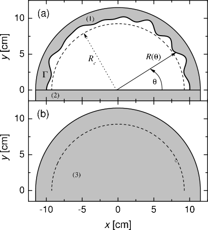
Figure 1: Upper panel: Sketch of the chaotic half-circular 3D microwave rough billiard in the $xy$ plane. Dimensions are given in cm. The cavity sidewalls are marked by 1 and 2 (see text). Squared wave functions $|\psi_{N,p}(R_{c},\theta)|^{2}$ were evaluated on a half-circle of fixed radius $R_{c}=9.25$ cm. Billiard’s rough boundary $\Gamma$ is marked with the bold line. Lower panel: White circle marks the position of the hole drilled in the upper wall of the cavity. This hole was used to introduce the perturber inside the cavity in order to measure the $z$-component of the electric field distributions $E_{N,p}({\bf x})$.

In the experiment we used 3D cavity with the translational symmetry in the shape of a rough half-circle (Fig. 1) with the height $h=60$ mm. The cavity was made of polished aluminium.

We suppose that the direction of the translational symmetry of the cavity is along the $z$-axis. The boundary conditions at $z=0$ and $z=h$ demand that the $z$ dependence of the $z$-component of the electric and magnetic fields $E_{N,p}({\bf x})$ and $B_{N,p}({\bf x})$ of TM modes be in the form $E_{N,p}({\bf x})\equiv E_{N,p}(x,y,z)=A_{N,p}\psi_{N,p}(x,y)f_{p}(z)$, where $f_{p}(z)=\cos(p\pi z/h)$, $p=0,1,2\ldots$, $A_{N,p}$ is the normalization constant and $B_{N,p}({\bf x})=0$. The functional dependence of $E_{N,p}({\bf x})$ on the plane cross section coordinates is denoted by the amplitude $\psi_{N,p}(x,y)\equiv E_{N,p}(x,y)$. The amplitude $\psi_{N,p}(x,y)$ satisfies the Helmholtz equation

$$(\bigtriangleup_{\bot}+k_{N,p}^{2})\psi_{N,p}(x,y)=0,$$

where $\bigtriangleup_{\bot}$ is two-dimensional Laplacian operator and $k_{N,p}=(k_{N}^{2}-(p\pi/h)^{2})^{1/2}$ is the effective wave vector. The wave vector $k_{N}=2\pi\nu_{N}/c$, where $\nu_{N}$ is the resonance frequency of the level $N$ and $c$ is the speed of light in the vacuum. The equation (1) is equivalent to the Schrödinger equation (in units $\hbar=1$) describing a particle of mass $m=1/2$ with the kinetic energy $k_{N}^{2}$ in an external potential $V=(p\pi/h)^{2}$ Kim2005 . Therefore, microwave 3D cavities with the translational symmetry simulate on the cross-sectional planes quantum billiards with the external potential $(p\pi/h)^{2}$. In this way microwave cavities can be effectively used beyond the standard 2D frequency limit (the case $p=0$) Hans in simulation of quantum systems. The amplitude $\psi_{N,p}(x,y)$ fulfills Dirichlet boundary conditions on the sidewalls of the billiard. Therefore, throughout the text the amplitudes $\psi_{N}(x,y)$ are also often called the wave functions $\psi_{N}(x,y)$. It is important to note that the full electric field $E_{N,p}({\bf x})$ satisfies additionally Neumann boundary conditions at the top and the bottom of the cavity.

Because of the relatively low quality factor of the cavity ($Q\simeq 4000$) the value of the level number $N$ was evaluated from the Balian–Bloch formula Balian

$$N(k)=\frac{1}{3\pi^{2}}Vk^{3}-\frac{2}{3\pi^{2}}\int_{S}\frac{d\sigma_{\omega}}{R_{\omega}}k,$$

where k is the wave vector, $V=(9.43\pm 0.01)\cdot 10^{-4}$ m³ is the volume of the cavity and $\int_{S}\frac{d\sigma_{\omega}}{R_{\omega}}=0.932$ m $\pm 0.005$ m is the surface curvature averaged over the surface of the cavity.

The measurements allowed us for the first time to evaluate the spatial correlation function Kaufman88

$$C_{N,p}({\bf x},{\bf s})=\frac{1}{\langle|E_{N,p}({\bf x})|^{2}\rangle}\langle E_{N,p}({\bf x}+\frac{1}{2}{\bf s})E_{N,p}^{\ast}({\bf x}-\frac{1}{2}{\bf s})\rangle,$$

where the local average $\langle\cdots\rangle$ is defined as follows

$$\langle|E_{N,p}({\bf x})|^{2}\rangle=\frac{1}{\Delta^{n}}\int_{-\Delta/2}^{\Delta/2}|E_{N,p}({\bf x}+{\bf s})|^{2}d^{n}s.$$

The 3D cavity sidewalls are made of 2 segments (see Fig. 1). The rough segment 1 is described on the cross-sectional planes by the radius function $R(\theta)=R_{0}+\sum_{m=2}^{M}{a_{m}\sin(m\theta+\phi_{m})}$, where the mean radius $R_{0}$=10.0 cm, $M=20$, $a_{m}$ and $\phi_{m}$ are uniformly distributed on [0.084,0.091] cm and [0,2$\pi$], respectively, and $0\leq\theta<{\pi}$. (Here, for the convenience, the polar coordinates $r$ and $\theta$ are used instead of the Cartesian ones $x$ and $y$.)

The surface roughness of a billiard on the cross-sectional planes is characterized by the function $k(\theta)=(dR/d\theta)/R_{0}$. For our billiard we have the angle average $\tilde{k}=(\left<k^{2}(\theta)\right>_{\theta})^{1/2}\simeq 0.400$. In such a billiard the classical dynamics is diffusive in orbital momentum due to collisions with the rough boundary because $\tilde{k}$ is much above the chaos border $k_{c}=M^{-5/2}=0.00056$ Frahm97 . The roughness parameter $\tilde{k}$ determines also other properties of the billiard Frahm on the cross-sectional planes. The amplitudes $\psi_{N,p}(r,\theta)$ are localized for the two-dimensional level number $N_{\bot}<N_{e}=1/128\tilde{k}^{4}$, where $N_{\bot}=\frac{A}{4\pi}k_{N,p}^{2}-\frac{P}{4\pi}k_{N,p}$. $A=(1.572\pm 0.002)\cdot 10^{-2}$ m² and $P=0.537$ m $\pm 0.001$ m are the cross-sectional plane area and its perimeter, respectively. Because of a large value of the roughness parameter $\tilde{k}$ the localization border lies very low, $N_{e}\simeq 1$. The border of Breit-Wigner regime is $N_{W}=M^{2}/48\tilde{k}^{2}\simeq 52$. It means that between $N_{e}<N_{\bot}<N_{W}$ Wigner ergodicity Frahm ought to be observed and for $N_{\bot}>N_{W}$ Shnirelman ergodicity should emerge.

To measure the amplitudes $\psi_{N,p}(r,\theta)$ of the 3D electric field distributions we used a very effective method described in Savytskyy2003 . It is based on the perturbation technique Slater52 and preparation of the “trial functions” Savytskyy2004 ; Hul2005 ; Hul2006 . In the perturbation method a small perturber is introduced inside the cavity to alter its resonant frequencies and in this way to evaluate the squared wave functions $|\psi_{N,p}(R_{c},\theta)|^{2}$ (see Fig.  1). The perturber (4.0 mm in length and 0.3 mm in diameter, oriented in $z$-direction) was moved by the stepper motor via the Kevlar line hidden in the groove (0.4 mm wide, 1.0 mm deep) made in the cavity’s bottom wall along the half-circle $R_{c}$. The measurements were performed at 0.36 mm steps along a half-circle with fixed radius $R_{c}=9.25$ cm.

In order to find the dependence of the electric field distributions $E_{N,p}({\bf x})$ on the $z$ coordinate and to estimate the wave vector $k_{3}=p\pi/h$ we measured the electric field inside the 3D cavity along the $z$-axis. Also in this case the perturber (4.5 mm in length and 0.3 mm in diameter) was attached to the Kevlar line and moved by the stepper motor. The perturber entered and exited the cavity by small holes (0.4 mm) drilled in the upper and the bottom walls of the cavity. The both holes were located at the position: $r=9.11$ cm, $\theta=0.47$ radians.

Using the method of the “trial wave function” we were able to reconstruct 75 experimental wave functions $\psi_{N,p}(r,\theta)$, which belonged to TM modes of the rough half-circular 3D billiard with the level number $N$ between 2 and 489. The range of corresponding eigenfrequencies was from $\nu_{2}\simeq 2.47$ GHz to $\nu_{489}\simeq 11.99$ GHz. The remaining wave functions belonging to TM modes, from the range $N=2-489$, were not reconstructed because of near-degeneration of the neighboring eigenfrequencies or due to the problems with the measurements of $|\psi_{N,p}(R_{c},\theta)|^{2}$ along a half-circle coinciding for its significant part with one of the nodal lines of $\psi_{N,p}(r,\theta)$.

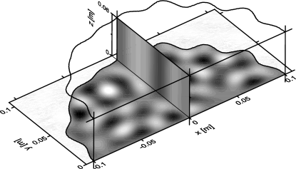
Figure 2: The reconstructed wave function $\psi_{460,0}(r,\theta)$ of the chaotic half-circular microwave rough billiard. The amplitudes have been converted into a grey scale with white corresponding to large positive and black corresponding to large negative values, respectively. Dimensions of the billiard are given in cm. In the figure the $z$ dependence of the electric field distribution $E_{460,0}(r,\theta,z)|_{x=0}\propto\psi_{460,0}(r,\theta)|_{x=0}f_{0}(z)$ is also shown.

In Fig. 2 and Fig. 3 we show two examples of reconstructed wave functions $\psi_{460,0}(r,\theta)$ and $\psi_{463,4}(r,\theta)$, respectively. The character of the wave functions predominantly depends on the effective wave vector $k_{N,p}$. It is seen that the wave function $\psi_{463,4}(r,\theta)$ in Fig. 3 is more regular than the one presented in Fig. 2 in spite of having the larger level number $N$.

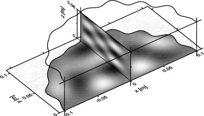
Figure 3: The reconstructed wave function $\psi_{463,4}(r,\theta)$ of the chaotic half-circular microwave rough billiard. The $z$ dependence of the electric field distribution $E_{463,4}(r,\theta,z)|_{x=0}\propto\psi_{463,4}(r,\theta)|_{x=0}f_{4}(z)$ is also shown.

In order to check ergodicity of the billiard’s wave functions $\psi_{N,p}(R_{c},\theta)$, especially close to the ergodicity borders, one should use some additional measures such as e.g., calculation of the structures of their energy surfaces Frahm97 . For this reason we extracted wave function amplitudes $C^{(N,p)}_{nl}=\left<n,l|N,p\right>$ in the basis $n,l$ of a half-circular billiard with radius $r_{max}$, where $n=1,2,3\ldots$ enumerates the zeros of the Bessel functions and $l=1,2,3\ldots$ is the angular quantum number. As expected, close to the border of the regimes of Breit-Wigner and Shnirelman ergodicity the wave function $\psi_{460,0}(r,\theta)$ ($N_{\bot}=65$) was found to be extended homogeneously over the whole energy surface Hlushchuk01 (figure not shown here). In contrary, the wave function $\psi_{463,4}(r,\theta)$, $N_{\bot}=16$, which lies closer to the localization boarder, displays the tendency to localization in $n,l$ basis (figure not shown here).

The measurement of 3D electric field distributions $E_{N,p}({\bf x})$ allowed us for the first time to find the experimental spatial correlation function $C_{N,p}({\bf x,s})$. It is easy to show Berry77 that for the 3D chaotic cavity with the translational symmetry the spatial correlation function should have the following form:

$$C_{N,p}({\bf x},|{\bf s}|)\equiv C_{N,p}(|{\bf s}|)=J_{0}(k_{N,p}s_{xy})\cos(p\pi s_{z}/h),$$

where $|{\bf s}|=(s_{xy}^{2}+s_{z}^{2})^{1/2}$. For the cross-sectional planes $z=const$ the correlation function $C_{N,p}(|{\bf s}|)\sim J_{0}(k_{N,p}s_{xy})$ is reduced to the well known result of Berry Berry77 for chaotic 2D wave functions described by a random superposition of plane waves.

Figure 4: Panels (a)-(c) show the experimental correlation function $C_{460,0}({\bf x},|{\bf s}|)$ calculated at ${\bf x}=$ (-2.75 cm, 4.35 cm, 0 cm) for the three projection angles $\phi=0$, $\pi/4$, and $\pi/2$, respectively. Experimental correlation function $C_{460,0}({\bf x},|{\bf s}|)$ (full line) is compared with the theoretical one (dashed line).

In Fig. 4(a)-(c) we show a representative example of the experimental correlation function $C_{460,0}({\bf x},|{\bf s}|)$ ($N_{\bot}=65$) calculated at ${\bf x}=$ (-2.75 cm, 4.35 cm, 0 cm) for the three different projection angles $\phi=0$, $\pi/4$, and $\pi/2$, respectively, where $\phi=\arcsin(s_{z}/|{\bf s}|)$. The local average $\langle\cdots\rangle$ required for the evaluation of $C_{N,p}({\bf x},|{\bf s}|)$ (see the formulas (3) and (4)) was calculated on the cross-sectional plane $xy$ in the range $\Delta/2=2\pi/k_{N,p}$. The experimental correlation functions $C_{460,0}({\bf x},|{\bf s}|)$ are compared in Fig. 4 with the theoretical ones. In all cases we find good agreement with the theoretical predictions given by the formula (5). Small discrepancies observed in Fig. 4(a) for $|{\bf s}|>1$ can be connected with the finiteness of the system and were theoretically studied in Baecker02 .

Figure 5: Panels (a)-(c) show the experimental correlation function $C_{463,4}({\bf x},|{\bf s}|)$ calculated at ${\bf x}=$ (-2.75 cm, 4.35 cm, 0 cm) for the three projection angles $\phi=0$, $\pi/4$, and $\pi/2$, respectively. Experimental correlation function $C_{463,4}({\bf x},|{\bf s}|)$ (full line) is compared with the theoretical one (dashed line).

Fig. 5(a)-(c) shows the experimental correlation function $C_{463,4}({\bf x},|{\bf s}|)$ ($N_{\bot}=16$) calculated at ${\bf x}=$ (-2.75 cm, 4.35 cm, 0 cm) for the three different projection angles $\phi=0$, $\pi/4$, and $\pi/2$, respectively. The experimental correlation functions $C_{463,4}(|{\bf s}|)$ are compared in Fig. 5 with the theoretical ones. In Fig. 5 (a), even for small $|{\bf s}|$, we find a significant departure of the experimental correlation function from the theoretical prediction, which clearly suggests that the wave function $\psi_{463,4}(r,\theta)$ is not chaotic. Also in Fig. 5 (b)-(c) the experimental correlation functions $C_{463,4}(|{\bf s}|)$ show for larger $|{\bf s}|$ significant deviations from the theoretical ones. The discrepancies between the correlation function $C_{463,4}({\bf x},|{\bf s}|=z)$ for the $z$-component of the electric field distribution and the theoretical prediction in Fig. 5(c) arise mainly due to the procedure of averaging of the correlation function $C_{N,p}({\bf x},|{\bf s}|)$ in $z$-direction, which was taken over the period of the cosine function.

In summary, we measured the wave functions of the chaotic 3D rough microwave billiard with the translational symmetry up to the level number $N=489$. For the first time the experimental correlation function $C_{N,p}({\bf x},{\bf s})$ was estimated and compared with the theoretical prediction. For the states with higher $N_{\bot}$ we find, especially for small values of the parameter $|{\bf s}|$, good agreement with the theoretical predictions, which show that the wave functions are chaotic. For the states with lower $N_{\bot}$ significant discrepancies between experimental and theoretical results are observed.

Acknowledgments. This work was partially supported by the Ministry of Science and Higher Education grants No. N202 099 31/0746 and 2 P03B 047 24.

References

- (1) S. Deus, P.M. Koch, and L. Sirko, Phys. Rev. E 52, 1146 (1995).
- (2) H. Alt, C. Dembowski, H.-D. Gräf, R. Hofferbert, H. Rehfeld, A. Richter, R. Schuhmann, and T. Weinland, Phys. Rev. Lett. 79, 1026 (1997).
- (3) U. Dörr, H.-J. Stöckmann, M. Barth, and U. Kuhl, Phys. Rev. Lett. 80, 1030 (1998).
- (4) B. Eckhardt, U. Dörr, U. Kuhl, and H.-J. Stöckmann, Europhys. Lett. 46, 134 (1999).
- (5) C. Dembowski, B. Dietz, H.-D. Gräf, A. Heine, T. Papenbrock, A. Richter, and C. Richter, Phys. Rev. Lett. 89, 064101 (2002).
- (6) H. Primack and U. Smilansky, Phys. Rev. Lett. 74, 4831 (1995).
- (7) T. Prosen, Phys. Lett. A 233, 323 (1997).
- (8) L. R. Arnaut, Phys. Rev. E 73, 036604 (2006).
- (9) Y.-H. Kim, U. Kuhl, H.-J. Stöckmann, and J. P. Bird, J. Phys.: Condens. Matter 17, L191 (2005).
- (10) H.-J. Stöckmann, J. Stein, Phys. Rev. Lett. 64, 2215 (1990).
- (11) R. Balian and C. Bloch, Ann. Phys. (N.Y.) 84, 559 (1974); Ann. Phys. (N.Y.) 64, 271(E) (1971).
- (12) S.W. McDonald and A.N. Kaufman, Phys. Rev A 37, 3067 (1988).
- (13) Y. Hlushchuk, A. Błȩdowski, N. Savytskyy, and L. Sirko, Physica Scripta 64, 192 (2001).
- (14) K.M. Frahm and D.L. Shepelyansky, Phys. Rev. Lett. 78, 1440 (1997).
- (15) K.M. Frahm and D.L. Shepelyansky, Phys. Rev. Lett. 79, 1833 (1997).
- (16) N. Savytskyy and L. Sirko, Phys. Rev. E 65, 066202-1 (2002).
- (17) L.C. Maier and J.C. Slater, J. Appl. Phys. 23, 68 (1952).
- (18) N. Savytskyy, O. Hul, and L. Sirko, Phys. Rev. E 70, 056209 (2004).
- (19) O. Hul, N. Savytskyy, O. Tymoshchuk, S. Bauch, and L. Sirko, Phys. Rev. E 72, 066212 (2005).
- (20) O. Hul, N. Savytskyy, O. Tymoshchuk, S. Bauch, and L. Sirko, Acta Phys. Pol. A 109, 73 (2006).
- (21) M.V. Berry, J. Phys. A 10, 2083 (1977).
- (22) A. Bäcker and R. Schubert, J. Phys. A 35, 539 (2002).