Coherent control of an effective two-level system in a non-Markovian biomolecular environment

Abstract

We investigate the quantum coherent dynamics of an externally driven effective two-level system subjected to a slow Ohmic environment characteristic of biomolecular protein-solvent reservoirs in photosynthetic light harvesting complexes. By means of the numerically exact quasi adiabatic propagator path integral (QUAPI) method we are able to include non-Markovian features of the environment and show the dependence of the quantum coherence on the characteristic bath cut-off frequency $\omega_{c}$ as well as on the driving frequency $\omega_{l}$ and the field amplitude $A$. Our calculations extend from the weak coupling regime to the incoherent strong coupling regime. In the latter case, we find evidence for a resonant behaviour, beyond the expected behaviour, when the reorganization energy $E_{r}$ coincides with the driving frequency. Moreover, we investigate how the coherent destruction of tunneling within the two-level system is influenced by the non-Markovian environment.

1 Introduction

During the past decade, a tremendous advancement in realizing and controlling the coherent quantum dynamics in solid-state nanosystems by an external time-dependent force has been achieved [1]. The theoretical description of driven quantum systems has discerned novel effects related to the control of quantum tunneling (see, e.g., [2] for a comprehensive review). Classical examples of the achieved degree of quantum control are the manipulation of trapped atoms in quantum optics [3] and the control of chemical reactions by external laser fields [2]. In quantum optics, it has been experimentally demonstrated that the time evolution of a two-level atom can be significantly modified by means of a frequency modulated excitation of the atom by use of a microwave field [4]. Moreover, it has been shown that tunneling of an initially localized state in a double well potential can be almost completely suppressed by a properly tailored external driving force [5]. In addition, the experimental demonstration of a quantum coherent dynamics in a superconducting flux qubit coupled to a superconducting quantum interference device (SQUID) has been reported [6].

In fact, the coherent dynamics of a quantum system is disturbed by contact with the environment [7, 8]. On the one hand, the phase of the quantum coherences is perturbed, which leads to decoherence [9], and on the other hand, energy transfer between the system of interest and the environment takes place, which gives rise to dissipation [7, 8]. Besides the fundamental theoretical interest in such quantum dissipative systems, a deep understanding of the various mechanisms leading to dissipation and decoherence is of interest in the context of quantum information processing [9, 10]. In view of the requirements expected to be met in the realization of a quantum computer [11], it is of the utmost importance to control and stabilize the coherent dynamics of the quantum system of interest. Indeed, various candidates for realizing the building blocks of small scale quantum information processors with nanoscale solid-state structures have been proposed [12, 13] and also partially realized in ground-breaking experiments [1].

To gain a deeper understanding of the quantum dissipative dynamics, a quantitative model including the effects of time-dependent driving, decoherence and dissipation is required. One generic model to investigate these effects is the time-dependent spin-boson model [2, 7], where the tunnel-splitting of the coherent two-level system (TLS) is usually denoted by $\Delta$. The environment is commonly described via the spectral density $J(\omega)$ [7]. In many cases, an Ohmic spectral density, where $J(\omega)\propto\omega$, occurs, as in the case of an unstructured electromagnetic environment, where all transitions within the system are equally damped [7].

To take into account the fact that the environmental frequencies are in principle limited, a high-frequency cut-off $\omega_{c}$ has to be introduced. This frequency scale is related to the time scale on which the environmental degrees of freedom evolve [7]. In many cases, $\omega_{c}$ is chosen to be the largest frequency scale in the problem ($\omega_{c}\gg\Delta$), which corresponds to the fact that the environmental fluctuations evolve on the shortest possible time scale, and hence the bath is ‘fast’. This describes, e.g., electromagnetic fluctuations in a crystal host [7, 14, 15] or in a superconductor [7]. Under this condition, a Markov assumption can be made yielding an effective time-local dissipative dynamics. This is also the regime in which Bloch-Redfield type master equations are commonly used [16], typically in connection with the additional assumption of weak system-bath coupling. The opposite case, when $\omega_{c}\ll\Delta$ describes an effective adiabatic bath which can be treated in a rather simplified manner [7]. There are, however, relevant situations when the bath fluctuations occur on a similar time scale on which the system evolves, i.e., $\omega_{c}\simeq\Delta$. This, for instance, typically occurs in the quantum coherent dynamics at the initial stage of photosynthesis in complex biomolecular structures [16, 17, 18, 19, 20]. It has only recently been experimentally hinted that the efficiency of the energy transfer from the light harvesting antenna complex to the chemical reaction center is promoted by the appearance of a quantum coherent dynamics [21, 22]. This hypothesis is further underpinned in [21, 22], where it has been evidenced that the collective long-range electrostatic response of the biomolecular protein environment to the electronic excitations should be responsible for the measured long-lived quantum coherences. In the experiment reported in [21], a quantum coherent excitonic dynamics in the energy transfer among bacteriochlorophyll (BChl) complexes over a time of around 660 fs has been measured at a temperature of 77 K. Such a dynamics is highly non-Markovian and more elaborate techniques have to be applied in order to provide an appropriate theoretical description.

In what follows, we consider an externally driven TLS subjected to an Ohmic environment with an exponential cut-off. Here, the focus is on the non-Markovian influence of a finite $\omega_{c}$ on the quantum coherent dynamics. The appropriate numerically exact tool to investigate non-Markovian dynamics is the quasi-adiabatic propagator path integral (QUAPI) method, which we briefly describe in section 2.3. We are able to investigate the entire parameter regime of weak as well as strong system-bath coupling situation beyond the often used scaling limit $\Delta\ll\omega_{c}$. We compare the weak coupling approximation based on a Born-Markov approach against the QUAPI method and show that the inclusion of non-Markovian effects is indeed necessary to obtain the correct result in the regime $\omega_{c}\simeq\Delta$ (section 3.1). The QUAPI method allows one to go far beyond the limiting cases within the Born-Markov approach, since all non-Markovian effects are exactly included.

The investigation of the parameter regime $\omega_{c}\sim\Delta$ is motivated by the fact that a slow environment is indeed of physical relevance to light-harvesting biomolecular complexes which are embedded in a polar solvent [20]. Here, we introduce a model for an effective TLS constructed from two interacting chromophores coupled to a protein-polar solvent reservoir. Furthermore, we drive the effective biomolecular TLS with an external laser and show that the Hamiltonian for the full system can be described in terms of the driven spin-boson model. The driven dissipative dynamics is investigated with the objective of understanding basic quantum interference phenomena which could be realized as proof-of-principle quantum coherent control experiments in light harvesting (LH) photosynthetic complexes such as LH II [16] or in artificially designed TLS nanostructures with specific bath properties. Only recently, we have demonstrated that in these systems a non-Markovian environment is most successful in generating entanglement of two non-interacting qubits which are coupled to the same Ohmic environment [23].

We compare our results for the undriven TLS with the outcome of real-time Monte Carlo simulations [24] and show that the QUAPI approach gives reliable results in the non-Markovian strong coupling case (section 3.2). In addition, we include an external time-dependent drive at frequency $\omega_{l}$ and show in section 3.3, for moderate and strong driving, that the amplitude of the forced oscillations in the stationary limit strongly depends on $\omega_{l}$ and, moreover, on $\omega_{c}$. Most interestingly, it turns out that a slow environment together with a slow drive $\omega_{l}$ optimizes the forced oscillations in the stationary limit. Finally, in section 3.4, the effect of a slow dissipative environment on the coherent destruction of tunneling in the TLS is investigated. We find that the bath influence is indeed strongest in the scenario $\omega_{c}\simeq\Delta$.

2 Model and method

2.1 Model for the dissipative TLS

The driven two-level system (TLS) bilinearly coupled to a bosonic heat bath is described by the generic spin-boson Hamiltonian [7]

$$H(t)=H_{S}(t)+H_{SB}+H_{B}\,.$$ (1)

Here, the system Hamiltonian $H_{S}(t)$ is chosen to be in the basis of the two states $|0\rangle$ and $|1\rangle$, each being, for example, the localized charge state of a charge qubit, or the ground state and the excited state of a two-level atom. The TLS, with the tunnel splitting $\Delta$, is driven by a time-dependent external driving field of the form $\varepsilon(t)=A\cos\left(\omega_{l}t\right)$ with amplitude $A$ and driving-frequency $\omega_{l}$ yielding

$$H_{S}(t)=\frac{\hbar}{2}\left(\Delta\sigma_{x}+\varepsilon(t)\sigma_{z}\right)\,,$$ (2)

with $\sigma_{i=x,z}$ being the Pauli pseudo-spin matrices. The environment to which the TLS is bilinearly coupled is modeled as a bath of harmonic oscillators with bosonic creation and annihilation operators $b^{\dagger},b$ and oscillator frequency $\omega_{\alpha}$, hence $H_{B}=\sum_{\alpha}\hbar\omega_{\alpha}b^{\dagger}_{\alpha}b_{\alpha}$. The coupling between the TLS and the environment is taken into account by the interaction Hamiltonian

$$H_{SB}=\frac{\hbar}{2}\sigma_{z}\sum_{\alpha}g_{\alpha}\left(b^{\dagger}_{\alpha}+b_{\alpha}\right)\,,$$ (3)

with $g_{\alpha}$ being the coupling constants.

2.2 Model for the dissipative photosynthetic light-harvesting effective TLS

Complex photosynthetic biomolecular structures have recently been shown to exhibit quantum interference properties [21, 22]. In particular, energy transfer among the excitons within chlorophyll complexes of the sulfur [21] and the purple [22] bacteria have provided evidence for long-lived (picosecond time scale) quantum coherent excitonic dynamics, a fact that has only recently become associated to the efficiency of the energy transfer from the LH antenna complexes to the chemical reaction centres in such large biomolecules [21, 22, 23].

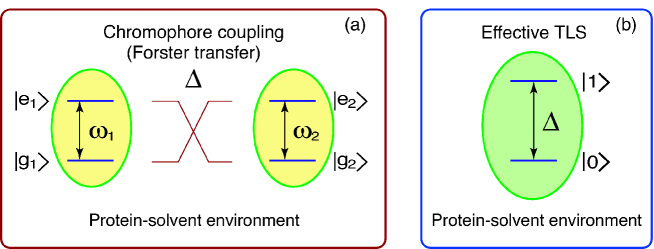
Figure 1: Sketch of the effective light harvesting biomolecular TLS formed from a pair of $\Delta-$Förster interacting chromophores.

In this work, we are interested in the dissipative dynamics of the minimal, basic unit of a photosynthetic LH complex which would allow us to model and control quantum interference mechanisms taking place in such nanostructures. This is done by modeling the specific case of an interacting pair of chromophores in a LH II ring [16]. The effective single TLS is built up from two chromophores which are coupled by the Förster resonant energy transfer $\Delta$, as sketched in figure 1(a), where $\hbar\omega_{j}$ is the transition energy for chromophore $j$. Since the fluorescence lifetime of the single chromophore is much larger than the other time scales of the system [20], no radiative decay of the excitations is taken into account, and we can write the Hamiltonian for the two-chromophore system in the basis ${\cal{B}}_{2}\equiv\{\left|g_{1}\right>\otimes\left|g_{2}\right>,\left|g_{1}\right>\otimes\left|e_{2}\right>,\left|e_{1}\right>\otimes\left|g_{2}\right>,\left|e_{1}\right>\otimes\left|e_{2}\right>\}$, where $g_{j}$ ($e_{j}$) corresponds to the ground (excited) state of chromophore $j$. The $\Delta$–Förster coupling between the two chromophores (figure 1(a)) comprises a dipole-dipole interaction which produces a non-radiative transfer of an excitation between the chromophores. Such an interaction can be written as $H_{int}=\frac{\hbar\Delta}{2}(\sigma_{x}^{1}\sigma_{x}^{2}+\sigma_{y}^{1}\sigma_{y}^{2})$, and the Hamiltonian of the bare system becomes

$$H_{S}=H_{1}\otimes\sigma_{0}^{2}+\sigma_{0}^{1}\otimes H_{2}+H_{int}\,,$$ (4)

where $\sigma_{0}^{i}$ is the identity matrix in the space of chromophore $i$.

The correlations due to the bath enter through the coupling to a surrounding protein environment and to a polar solvent, which, in general, exhibits a frequency dependent dielectric constant [25]. For the details of such a mechanism and their possible geometric configurations, we refer to [25]. Formally, this process can be modeled by means of a quantized reaction field operator $R^{i}\equiv\sum_{\alpha}D_{\alpha}^{i}(b_{i,\alpha}+b_{i,\alpha}^{\dagger})$, where $D_{\alpha}^{i}$ couples the chromophores $i$ to the surrounding environment. This, in turn, is modeled as a bath of harmonic oscillators which comprise the energy stored in the polar solvent. Such modes are represented via the bosonic operators $b_{\alpha}$, and, as in the previous section, the bath Hamiltonian reads $H_{B}=\sum_{\alpha}\hbar\omega_{\alpha}b_{\alpha}^{\dagger}b_{\alpha}.$ If $\delta\mu_{i}$ denotes the change in the dipole moment of molecule $i$ during the transition [20], i.e., the difference between the dipole moment of the chromophore in the ground and excited states, the two chromophores are coupled to their environment via the interaction Hamiltonian

$$H_{SB}=\frac{\hbar}{2}\left[\left(\delta\mu_{1}\sigma_{z}^{1}\sum_{\alpha}D_{\alpha}^{1}(b_{\alpha}+b_{\alpha}^{\dagger})\right)\otimes\sigma_{0}^{2}+\sigma_{0}^{1}\otimes\left(\delta\mu_{2}\sigma_{z}^{2}\sum_{\alpha}D_{\alpha}^{2}(b_{\alpha}+b_{\alpha}^{\dagger})\right)\right]\,.$$

The total Hamiltonian for the two-chromophores is then written in the basis ${\cal{B}}_{2}$ as

$$H = H_{S}+H_{B}+H_{SB}=$$

$$= \sum_{\alpha}\hbar\omega_{\alpha}b_{\alpha}^{\dagger}b_{\alpha}+\frac{\hbar}{2}\left(\begin{array}[]{cccc}-\left(\Omega_{+}+V_{+}\right)&0&0&0\\[5.69054pt] 0&-\left(\Omega_{-}+V_{-}\right)&2\Delta&0\\[5.69054pt] 0&2\Delta&\Omega_{-}+V_{-}&0\\[5.69054pt] 0&0&0&\Omega_{+}+V_{+}\end{array}\right)\,,$$

where $\Omega_{\pm}\equiv\omega_{1}\pm\omega_{2}$, and $V_{\pm}\equiv\delta\mu_{1}R^{1}\pm\delta\mu_{2}R^{2}$. Given the biophysical nanostructure composition of the LH II rings [16], we assume that the states of the single chromophores couple to the same surrounding protein bath. Consequently we set $D\equiv D^{1}=D^{2}$, and drop any subscripts that may differentiate the bath modes associated to chromophores 1 and 2 in $H_{B}$.

If only singly excited states are taken into account, from the Hamiltonian (2.2) we identify the active environment coupled 2D-subspace $\{|e_{1}\rangle\otimes|g_{2}\rangle,|g_{1}\rangle\otimes|e_{2}\rangle\}$. In this central subspace of (2.2), the effective interacting biomolecular TLS Hamiltonian reads

$$H=\left(\frac{\hbar\Omega}{2}\sigma_{z}+\hbar\Delta\sigma_{x}\right)+\frac{\hbar}{2}\sigma_{z}\sum_{\alpha}g_{\alpha}\left(b_{\alpha}+b^{\dagger}_{\alpha}\right)+\sum_{\alpha}\hbar\omega_{\alpha}b_{\alpha}^{\dagger}b_{\alpha}\ ,$$ (8)

with $g_{\alpha}\equiv D_{\alpha}(\delta\mu_{1}-\delta\mu_{2})$ being the bath coupling constants, and $\Omega\equiv\Omega_{-}$. Now the defined effective biomolecular TLS has tunneling splitting $\Delta$; if, as before, such a TLS is driven by a time-dependent external driving field $\varepsilon(t)=A\cos\left(\omega_{l}t\right)$, and we consider that both chromophores have equal transition energies ($\omega_{1}=\omega_{2}$), the Hamiltonian (8) becomes equal to the total Hamiltonian $H(t)$ (1), and hence we have effectively mapped the interacting, environment correlated chromophore system Hamiltonian to that of a generic effective spin-boson Hamiltonian. This is esquematically illustrated in figure 1(b), where $\Delta$ is the associated “tunneling energy”, between the new basis states $\left|0\right>$ and $\left|1\right>$ for the effective biomolecular TLS (formerly the ${\cal{B}}_{2}$–basis states $\left|ge\right>$ and $\left|eg\right>$, respectively).

To gain information on the full dynamics of the system, the initial conditions at $t=0$ have to be specified. In all our simulations we assume that the full density matrix $\rho$ at the initial time $t=0$ factorizes in accordance with

$$\rho(0)=\rho_{S}(0)\otimes\rho_{B}\,.$$ (9)

Here, $\rho_{S}(0)$ is the density matrix of the TLS at initial time $t_{0}=0$ and the decoupled bath canonical distribution $\rho_{B}=\mbox{Z}_{B}\exp(-H_{B}/k_{B}T)$, where $\mbox{Z}_{B}=\tr\exp(-H_{B}/k_{B}T)$. To keep the bath in thermal equilibrium, the bath is coupled to a not further specified super-bath at temperature $T$.

The environment is fully characterized by the spectral density $J(\omega)=\sum_{\alpha}g_{\alpha}^{2}\delta(\omega-\omega_{\alpha})$, being a quasi-continuous function for typical condensed phase applications. It determines all bath-correlations that are relevant for the system via the bath auto-correlation function [7, 26]

$$L(t)=\frac{1}{\pi}\int\limits_{0}^{\infty}d\omega J(\omega)\left[\coth\frac{\hbar\omega}{2k_{B}T}\cos\omega t-i\sin\omega t\right]\,.$$ (10)

We emphasize at this point that within our numerical method (see below) the full structure of $L(t)$ is included, which is essential to describe non-Markovian features of the system dynamics. In particular, we avoid the often used Born-Markov approximation, which consists of replacing the real part of $L(t)$ by a $\delta$-function and neglecting its imaginary part.

For what is reported in the following, we use an Ohmic spectral density with an exponential cut-off, i.e.,

$$J(\omega)=2\pi\alpha\omega\exp(-\omega/\omega_{c}),$$ (11)

where the dimensionless parameter $\alpha$ describes the damping strength and $\omega_{c}$ is the cut-off frequency. An Ohmic spectral density is a proper choice for, e.g. electron transfer dynamics [24, 27] or biomolecular complexes [16, 20, 23], as well as in the case of Josephson junction qubits [28]. In the case of charge qubits subjected to a phonon bath, a different spectral density, with a super-Ohmic low-frequency behaviour, results better suited [14, 15].

A microscopic derivation for the spectral density associated to the bacteriochlorophylls in the LH II complexes considered in this work has been reported in [25], where different forms of a Debye dielectric solvent have been considered. In general, they lead to the Ohmic type of spectral density given by (11). The dimensionless damping constant $\alpha$ of the protein-solvent is directly related to the parameters of the dielectric model [25], and has been estimated to be in the range $\alpha\sim 0.01-1$ [20, 25]. The exponential decay of the high-frequency cut-off $\omega_{c}$ sets the bath characteristic time-scale. If $\Delta\ll\omega_{c}$, the bath is very fast compared to the effective TLS and loses its memory quickly. Here, a Markovian approximation is appropriate and the standard Bloch-Redfield description [16] applies. However, for the considered biomolecular environment, $\hbar\omega_{c}$ is typically of the order of $\sim 2-8$ meV, while the Förster coupling strengths $\hbar\Delta\sim 0.2-100$ meV [20, 25]. Hence, the bath responds slower than the dynamics of the excitons evolve and non-Markovian effects become dominant, a regime which is accessible only by rather advanced techniques.

Below, we report results in the scaling limit $\Delta,T\ll\omega_{c}$ and vary $\omega_{c}$ such that the system reaches the crossover to the adiabatic limit, i.e., $\omega_{c}\sim\Delta$. Both regimes, and the associated crossover, have been studied by real-time Quantum Monte Carlo simulations for electron transfer dynamics within the undriven TLS for selected parameter combinations [24]. In this work, we go beyond this by including an external laser driving and, furthermore, by covering the entire parameter space. Concerning the coupling between the TLS and its environment, we study the whole parameter window from the weak coupling limit $\alpha\ll 1$ to the strong coupling limit $\alpha\sim 1$.

2.3 The quasi-adiabatic propagator path integral method

The dynamics of the TLS introduced in the previous section is described in terms of the time evolution of the reduced density matrix $\rho(t)$ which is obtained by tracing over the bath degrees of freedom. The TLS dynamics always evolves from the initial state $\rho_{S}(0)=\left|1\right>\left<1\right|$.

In order to investigate the dynamics of the system, we use the QUAPI scheme [29], which is a numerically exact iteration scheme which has been successfully adopted to many problems of open quantum systems [14, 23, 30]. For details of the iterative scheme we refer to previous works [29, 30] and do not reiterate them here.

The algorithm is based on a symmetric Trotter splitting of the short-time propagator $K(t_{k+1},t_{k})$ of the full system into a part depending on $H_{S}$ and $H_{B}+H_{SB}$ describing the time evolution on a time slice $\delta t$. This is exact in the limit $\delta t\to 0$ but introduces a finite Trotter error to the propagation which has to be eliminated by choosing $\Delta t$ small enough that convergence is achieved. On the other side, the bath-induced correlations being non-local in time are included in the numerical scheme over a finite memory time $\tau_{mem}=K\delta t$ which roughly corresponds to the time range over which the bath auto-correlation function $L(t)$ given in (10) is significantly different from zero. As the environmental fluctuations live on a time scale $\sim 1/\omega_{c}$, it is particularly important to include the full memory when $\omega_{c}\simeq\Delta$. Note that for any finite temperature, $L(t)$ decays exponentially at long times [7], thus justifying this approach. Moreover, $K$ has to be increased, until convergence with respect to the memory time has been found. Typical values, for which convergence can be achieved for our spin-boson system, are $K\leq 12$ and $\delta t\sim(0.1-0.2)/\Delta$. The two strategies to achieve convergence are countercurrent. To solve this, the principal of least dependence has been invoked [30] to find an optimal time increment in between the two limits $K\to\infty$ and $\delta t\to 0$.

3 Dynamics of the driven TLS

With the time evolution of the reduced density matrix $\rho(t)$ at hand we can now study the dynamics of the driven TLS in terms of the population difference $P(t)=\langle\rho(t)\sigma_{z}\rangle$ of the two states, with the initial condition $P(0)=1$.

3.1 Markovian vs non-Markovian dynamics

Before addressing the effect of driving, we convince ourselves that the dynamics is indeed non-Markovian when $\omega_{c}\simeq\Delta$. For this, we compare the numerical exact QUAPI with a Bloch-Redfield approach. To be specific, we compare the QUAPI data with the outcome of the weak coupling approximation, see (21.171) and (21.172) in [7], which results from a first order approximation in $\alpha$. In [31], it has been shown that the outcome of the weak coupling approach is equivalent to a Bloch-Redfield treatment.

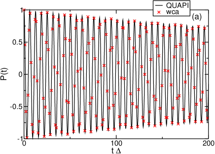
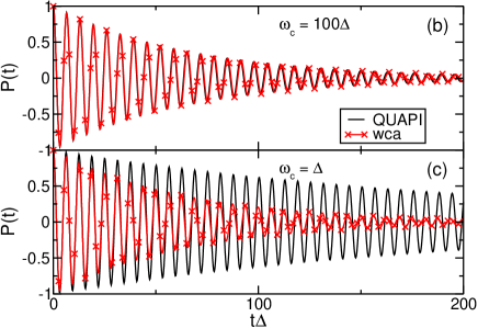
Figure 2: Population difference $P(t)$ for the undriven spin-boson model $A=0$ (solid line: QUAPI, symbols: weak coupling approach). (a) $\alpha=0.001$ and $\omega_{c}=100\Delta$ (Markovian regime), (b) $\alpha=0.01$ and $\omega_{c}=100\Delta$, and (c) $\alpha=0.01$ and $\omega_{c}=\Delta$. The temperature is always $T=10\Delta$.

In figure 2 (a) the result for $\alpha=0.001$ and $\omega_{c}=100\Delta$ is shown. As expected, the agreement between both results is perfect since the system is deep in the Markovian (weak coupling) regime. For figure 2 (b) the coupling is increased to $\alpha=0.01$ and since the bath is still in the scaling limit there is acceptable agreement. In contrast, for a cut-off frequency $\omega_{c}=\Delta$, see figure 2 (c), strong deviations between the Bloch-Redfield approach and the QUAPI approach arise, indicating that the environment is non-Markovian in nature here. Although the smooth cut-off function with the reduced spectral weight at frequencies $\omega\sim\omega_{c}>\Delta$ is fully included within the Bloch-Redfield approach, we see strong deviations. This further underpins that, as expected, the Bloch-Redfield approach fails when the bath fluctuates on a time scale comparable to that of the system’s time evolution.

When the damping is furthermore increased to $\alpha=0.1$ the disagreement between the numerical exact QUAPI and the weak coupling approximation is enhanced, see figs. 3 (a) and (b). This indicates that the choice of $\omega_{c}$ away from the scaling limit induces a non-Markovian behaviour of the dissipative TLS dynamics which is further underpinned by figure 3 (c), where the relaxation rate $\gamma_{r}$ is shown. We obtain this from a fit of a decaying cosine function with a single exponential to $P(t)$. In the scaling limit $\Delta\ll\omega_{c}$ both approaches yield the same $\gamma_{r}$, whereas strong deviations occur for smaller $\omega_{c}$. Note that $\omega_{c}$ enters (21.171) in [7] via the renormalized tunneling amplitude $\Delta_{\rm eff}$ which is included here in the weak-coupling approximation.

3.2 Undriven case: comparison with Quantum Monte Carlo results

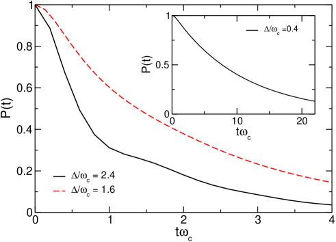
Figure 4: Population difference $P(t)$ for the TLS for different cut-off frequencies $\omega_{c}$ and a damping parameter $\alpha=2$. The temperature $T=4\omega_{c}$ (main), and $T=0.4\omega_{c}$ (inset).

Next, in order to validate our results in the highly non-Markovian crossover regime $\omega_{c}\sim\Delta$, we compare our results with the outcome of real-time Quantum Monte Carlo (QMC) simulations [27]. In figure 4 (main), the results for the high temperature regime are shown, where the parameters are $T=4\omega_{c}$ and $\alpha=2$ (strong coupling). In perfect (also quantitative) agreement with [27], $P(t)$ decreases faster for $\Delta/\omega_{c}=2.4$ than for $\Delta/\omega_{c}=1.6$. The cut-off frequency is also related to the reorganization energy of the environment [7], which has the form $E_{r}=\int_{0}^{\infty}d\omega\frac{J(\omega)}{\pi\omega}=2\alpha\hbar\omega_{c}$ for an Ohmic environment. Hence, our results are consistent with the physical expectation, since the dynamics of the environment is slower for the smaller ratio $\Delta/\omega_{c}$ for the same $\alpha$. For the low temperature regime $T=0.4\omega_{c}$, shown in the inset of figure 4, we also observe agreement of the QUAPI results with the outcome of [27].

Furthermore, we address the case of strong coupling between the TLS and its environment. For the scaling limit $\Delta\ll\omega_{c}$ it is known that there is a transition at $\alpha=0.5$ from a coherent decay of $P(t)$ for $\alpha<0.5$ to an incoherent decay for $\alpha>0.5$ [7, 32]. To be specific, we choose $\alpha=0.6$ at a low temperature $T=0.1\Delta$, as shown in figure 5. Again, this behaviour can be understood in terms of the reorganization energy $E_{r}$, since decreasing $\omega_{c}$ here has a similar effect as lowering the damping parameter $\alpha$. By means of our numerical exact method, figure 5 quantifies how the transition between coherent and incoherent behaviour depends on $\omega_{c}$ for a given $\alpha$.

We next put our results in the context of the modeled effective biomolecular TLS. For excitations in the LH-II ring of the bacteria chlorophyl molecule (BChls in LH-II complexes), the Förster coupling strength $\hbar\Delta\sim 46-100$ meV, and $\hbar\omega_{c}\sim 2-8$ meV [20, 25], and hence the ratio $\frac{\omega_{c}}{\Delta}\sim 0.1$. For these complexes, $\alpha$ is of the order of $0.1-1$ [25], evidencing a strong coupling between the chromophores and the solvent dielectric. If we make $\alpha=0.1$, $\hbar\Delta=100$ meV, and plot a graph such as the one of figure 5 for $T=0.1\Delta$ ($\sim 116$ K), long-lived coherent oscillations are sustained for a time of around 530 fs ($t\Delta\sim 80$). Such oscillations can be visualized at fixed $\omega_{c}=0.1\Delta$ (not shown). This rough estimation is in agreement with the time scale of the coherent oscillations recently measured in [21] for the antenna complex from a green sulphur bacteria that has seven BChls per protein subunit. If, on the other hand, we make $\alpha=0.6$, $\omega_{c}=0.1\Delta$ (as shown in figure 5), coherent oscillations are also found but, due to the stronger coupling to the bath, they decay quicker than for the case $\alpha=0.1$. We thus observe that for the rather simple effective biomolecular TLS model introduced here, which is aimed as a guide to the possible realization of further proof-of-principle experiments, we are able to demonstrate that the non-Markovian features of the protein-solvent environment help to sustain the quantum coherence mechanisms exhibited by the coupled chromophores in a LH-II ring. Since our results are of a general character, in principle derived from a generic TLS, we also expect them to be valid in artificially designed nanostructures with the specific bath properties described here.

3.3 Driven case $A\neq 0$

We now address the influence of a finite periodic external driving field. The results for $A=\Delta$ and $\omega_{l}=0.05\Delta$ are shown in figure 6. Similarly to the undriven case, the overall decay of $P(t)$ is faster for larger $\omega_{c}$: compare, for example, figure 6 (a) for $\omega_{c}=1.5\Delta$ and figure 6 (b) for $\omega_{c}=30\Delta$, both in the weak-coupling situation $\alpha=0.01$. In turn, for the case $\omega_{c}\sim\Delta$, the superimposed oscillations due to coherent tunneling survive longer than in the scaling-limit $\Delta\ll\omega_{c}$ (figure 6(b)), before the system reaches its stationary state. There, only the stationary oscillations due to the external driving field survive. For a stronger system-bath coupling $\alpha$ the decay of $P(t)$ is faster, as expected, and the stationary state is reached faster (not shown). As in the undriven case, the described behaviour is qualitatively understandable in terms of the reorganization energy $E_{r}$.

For increasing driving strength to $A=10\Delta$, the dependence of the TLS dynamics on $\omega_{c}$ and $\alpha$ is similar. However, the form of the stationary oscillations turns out to be qualitatively different from the case of weak driving $A=\Delta$. Here, stable stationary plateaus emerge, as shown in figure 7. In [4], this has been observed experimentally for frequency-modulated excitations of a two-level atom, using a microwave field to drive transitions between two Rydberg-Stark states of potassium. In the presence of a slow frequency modulation, square wave oscillations of the population difference have been detected. They can be understood to mean that the large driving amplitude leads to an extreme biasing of the TLS dynamics. The centres of the observed plateaus correspond to the extrema of the applied cosine driving field. At the position of these maxima, the TLS is maximally biased and since the time-scale of the driving field is much smaller than the time-scale of the (unbiased) TLS dynamics due to $\Delta$, the situation of an extreme quasistatic bias results, forming an intermediate self-trapping around the maxima of the cosine-like driving field. Indeed, this intermediate self-trapping becomes shorter lived, and increasingly washed out, when the $\omega_{l}\sim\Delta$ (not shown here). For smaller $\alpha$ (figure 7a), the square wave form is superimposed by fast ”intrawell” damped oscillations which die out on a time scale $\sim 1/\alpha$. For increasing $\alpha$ (figure 7b), the fast “intrawell” oscillations are not present anymore and stable plateaus form immediately after the “interwell” transition. Due to the strong damping, the level is also strongly broadened and the quasistationary picture applies in which the level position is given by the mean energy of the broadened level. This is not so much sensitive anymore to further variation within a half period of the cosine field.

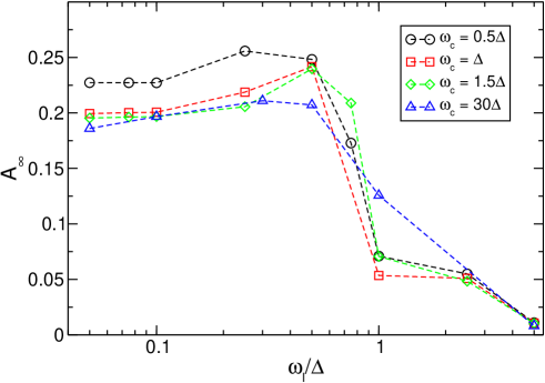
Figure 8: Amplitude of the forced oscillations in the stationary limit $A_{\infty}$ as a function of the driving frequency $\omega_{l}$, for $A=\Delta$ with $\alpha=0.1$ and different cut-off frequencies $\omega_{c}$.

In a next step, it is interesting to consider the amplitude $A_{\infty}$ of the forced oscillations in the stationary limit. In figure 8, we show the results for the nonlinear response for the case $\alpha=0.1$ and a driving field amplitude $A=\Delta$. We observe a rather weak dependence on $\omega_{l}$ when $\omega_{l}\lesssim\Delta$. Moreover, the response also becomes rather weak in the regime of strong detuning. In between these two regimes, we find an optimal driving frequency $\omega_{l}\sim\Delta/2$, where the amplitude of the forced oscillations has a maximum. Note that this rather weak resonance is due to the sizeable damping $\alpha=0.1$. The maximum can be related to the picture of quantum stochastic resonance in an unbiased but strongly damped bistable system [33]. The response of the system becomes optimal when the dissipative tunneling transitions are in synchrony with the external drive. In addition to this well known mechanism, we study here the dependence on the bath cut-off frequency. The behaviour depicted in figure 8 is, essentially, not influenced by $\omega_{c}$ for this value of the driving strength $A$ and is thus independent of the time scale of the environment (up to small quantitative modifications).

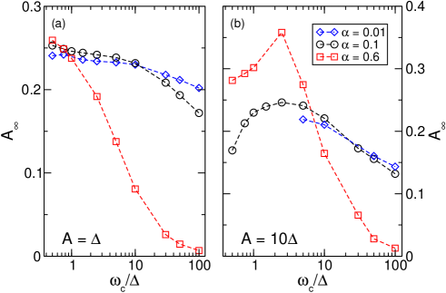
Figure 9: Amplitude $A_{\infty}$ of the forced stationary oscillations as a function of the cut-off frequency $\omega_{c}$ for (a) weak to intermediate driving $A=\Delta$, and (b) strong driving $A=10\Delta$, for three different values of $\alpha$. The remaining parameters are $\omega_{l}=0.5\Delta$, and $T=0.1\Delta$.

A natural question is whether to expect an enhancement of the response when all frequencies are comparable, i.e., $\omega_{l}\sim\omega_{c}\sim\Delta$. This situation is addressed in figure 9, where we have chosen $\omega_{l}=0.5\Delta$. We find that for weak to intermediate driving, no pronounced resonance appears, as shown in figure 9 (a) for the case $A=\Delta$. In contrast, strong driving can induce a resonant nonlinear response which, however, requires non-Markovian dynamics, i.e., $\omega_{c}\sim\Delta$. This is illustrated in figure 9 (b) for $A=10\Delta$. A slow non-Markovian bath with $\omega_{c}\lesssim\Delta$ is thus much more efficient in maximizing forced oscillations in the stationary limit. This feature occurs for the weak coupling ($\alpha=0.01$) as well as for the strong coupling case $\alpha=0.6$. This constitutes another example where a non-Markovian bath helps in increasing coherence in the quantum system [23].

In contrast, a Markovian environment in the scaling limit, $\Delta\ll\omega_{c}$, largely suppresses forced oscillations via its destructive influence on coherence. This finding is most pronounced in the incoherent strong coupling case, $\alpha=0.6$. The dependence of $A_{\infty}$ on $\omega_{c}$ is again qualitatively understandable via the reorganization energy $E_{r}$ in the case of weak driving. It explains the reduction of the response for weaker damping ($\alpha=0.1$ and $\alpha=0.01$), compared to the strong damping case $\alpha=0.6$ (figure 9 (a)). However, for stronger driving, $A=10\Delta$, the resonance effect is more pronounced for a strong coupling situation, $\alpha=0.6$ which cannot be explained in terms of a growing reorganization energy $E_{r}$.

3.4 Coherent destruction of tunneling

When an isolated symmetric quantum TLS is driven with large frequencies $\omega_{l}\gg\Delta$, the bare tunneling matrix element effectively becomes renormalized by the zero-th Bessel function $J_{0}(x)$ as $\Delta\rightarrow J_{0}(A/\omega_{l})\Delta\equiv\Delta_{\rm eff}$ [2, 34]. The population of the state $\left|1\right>$ with an initial preparation $\left|1\right>=1$ follows as

$$P_{1}(t)=\cos^{2}\left(J_{0}(a/\omega_{l})\Delta t/2\right)\,.$$ (12)

This implies that for particular choices of the driving parameters, the Bessel function term can be fixed to zero. The first zero then corresponds to $A/\omega_{l}=2.40482...$, and then, $P_{L}(t)$ equals unity, since the effective tunnel splitting vanishes. This phenomenon is known as coherent destruction of tunneling (CDT); see [2] and references therein for further details.

Naturally, the phenomenon of CDT is influenced when the TLS is coupled to an Ohmic environment. A complete standstill of the dynamics will no longer occur, due to the relaxation processes induced by the bath. For an Ohmic environment in the scaling limit under the assumption of weak damping, this question has been addressed in [35]. Here, the QUAPI technique allows us to extend these studies to the case of finite $\omega_{c}$. To be specific, we choose a driving frequency $\omega_{l}=20\Delta$.

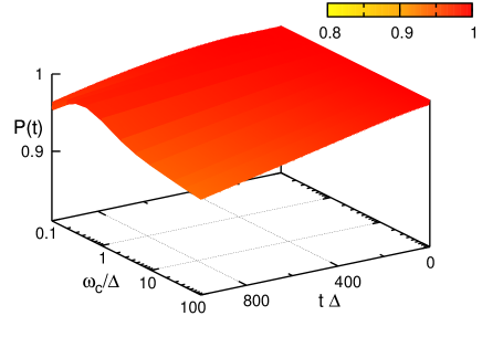
(b)

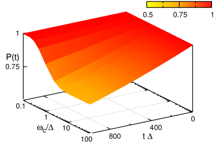
Figure 10: Population difference $P(t)$ for the driven TLS under the condition for coherent destruction of tunneling, $\omega_{l}=20\Delta,A=2.40\Delta$. The temperature $T=0.1\Delta$, and the damping is (a) $\alpha=0.01$, and (b) $\alpha=0.1$.

For weak coupling, $\alpha=0.01$, the CDT is only weakly influenced by the environment, as expected, and it turns out that the dependence on the cut-off frequency of the bath $\omega_{c}$ is also weak, as shown in figure 10 (left). Nevertheless, we find that the unavoidable decay of $P(t)$ occurs the slowest when $\omega_{c}\sim\Delta$. For stronger coupling $\alpha=0.1$, as shown in figure 10 (right), CDT is more strongly influenced by the magnitude of $\omega_{c}$. We observe, again, that a slow bath helps to preserve coherence and the decay of $P(t)$ is slow.

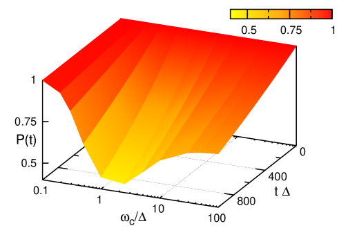
Figure 11: Same as figure 10, but for a strong coupling situation, $\alpha=0.6$.

In the regime of strong damping, the situation is different. In fact, we find an opposite qualitative behaviour which goes beyond the above given explanation in terms of $E_{r}$. In figure 11, the corresponding results for $\alpha=0.6$ are shown. As one can see, the decay of $P(t)$ is the fastest when $\omega_{c}\simeq\Delta$. This stems from the fact that for $\omega_{c}\sim\Delta$, non-Markovian effects are not negligible, since the time-scales of system and environment are of the same order, which is reflected in the fact that the spectral density $J(\omega)$ has a maximum around $\Delta$. In this resonant situation, the bath modes around the characteristic time scale $1/\Delta$ of the TLS are most important and disturb the CDT in a maximal (resonant) way. Consequently, the decay under the CDT conditions is most pronounced. In turn, in the scaling limit, the decay under CDT conditions is slow. Interestingly, in both cases of strong coupling ($\alpha=0.1;0.6$) the population difference is almost maintained on the considered time windows without decay by the slow bath $\omega_{c}\sim 0.1\Delta$, and the decay of $P(t)$ is the slowest.

4 Conclusion

We have investigated the dynamics of the driven spin-boson system in the presence of an Ohmic bath. The focus is put on the role of the cut-off frequency $\omega_{c}$. Based on the numerical exact QUAPI approach, non-Markovian effects are shown to be relevant when $\omega_{c}\sim\Delta$. This effect is more pronounced for strong damping, as expected, and as can be seen from the relaxation rate $\gamma_{r}$ shown in figure 3. The validity of the QUAPI method in the regime $\omega_{c}\sim\Delta$ is confirmed by the perfect agreement with published results of real time Quantum Monte Carlo simulations [24].

For the unbiased case and for strong coupling, we show that damped coherent oscillations exist in the population difference $P(t)$ if the bath has a cut-off frequency away from the scaling limit, where the decay is known to be incoherent in nature, as shown in figure 5. By comparison with relevant experimental data, we were able to show that our results are directly applicable to biomolecular systems, namely to the light harvesting complex LH-II of the bacteria chlorophyl molecule. We have shown that a sub-unit of such a biomolecular system can effectively be described by means of the spin-boson model and have demonstrated that the non-Markovian features of the protein-solvent environment help to sustain the quantum coherence mechanisms exhibited within the LH-II complex. Moreover, since our results are based on a model of general character, we expect them to apply also for a variety of artificially designed nanostructures with the specific bath properties reported here.

Regarding the coherent control of the effective TLS, we found that a strong external driving amplitude in combination with a slow driving laser frequency produce a population difference with square wave oscillations in the stationary limit, in agreement with the experimental results reported in [4]. These square-wave like oscillations stem from the fact that the TLS experiences a large quasistatic bias. Moreover, it was shown that the amplitude $A_{\infty}$ of the forced oscillation in the stationary limit depends strongly on the frequency of the driving field. A slow driving $\omega_{l}\lesssim\Delta$ field protects the forced oscillations against the influence of the dissipative environment, whereas in the case of a faster driving, these oscillations are strongly suppressed. This is valid for the weak-coupling as well as for the strong coupling case. For larger driving frequencies, the forced stationary oscillations are considerably reduced. The stationary amplitude of the forced oscillations also strongly depends on the time-scale of the environment determined by $\omega_{c}$. For strong driving, we find that the stationary amplitude shows resonant features, illustrating that the non-Markovian environment plays a constructive role.

Finally, we investigated the phenomenon of coherent destruction of tunneling under the bath influence. Away from the scaling limit, the influence of the environment is weaker and the CDT survives on a significantly longer time scale. For very strong coupling, i.e., deep in the incoherent regime, the situation is completely different. Here, the CDT is most quickly destroyed when the time scales of the TLS and the environment are in resonance. In such a strong coupling scenario, the preservation of coherence survives longer in the scaling limit; moreover, the CDT is actually helped by the effect of a slow bath (e.g., $\omega_{c}\sim 0.1\Delta$), where the decay of $P(t)$ is the slowest.

References

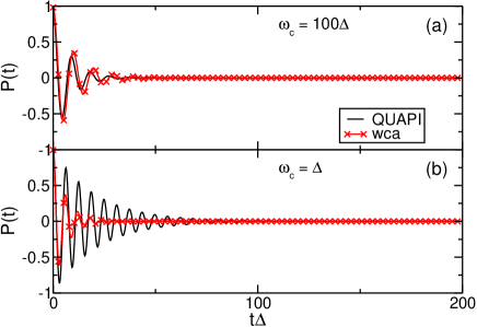
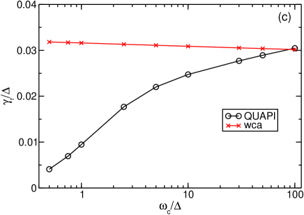
Figure 3: Same as figure 2, but for a strong coupling $\alpha=0.1$. (c) shows the relaxation rate $\gamma_{r}$ as a function of $\omega_{c}$.

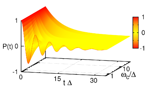
Figure 5: Population difference $P(t)$ for the undriven TLS system in dependence on the cut-off frequency $\omega_{c}$. The temperature $T=0.1\Delta$, and the damping parameter is $\alpha=0.6$.

Figure 6: Population difference $P(t)$ for the driven TLS. The amplitude of the driving-field is $A=\Delta$ and the driving-frequency is $\omega_{l}=0.05\Delta$. The temperature $T=0.1\Delta$, and the damping parameter $\alpha=0.01$. The cut-off frequency is (a) $\omega_{c}=1.5\Delta$ and (b) $\omega_{c}=30\Delta$

Figure 7: Population difference $P(t)$ for the driven single qubit system. The amplitude of the driving-field $A=10\Delta$, the driving-frequency $\omega_{l}=0.05\Delta$, the cut-off frequency $\omega_{c}=0.5\Delta$, and the temperature $T=0.1\Delta$. The damping parameter is (a) $\alpha=0.1$, and (b) $\alpha=0.6$.

(a)

References

- [1] For a review, see the Focus Issue on Solid State Quantum Information, edited by Fazio R 2005 New J. Phys.7
- [2] Grifoni M and Hänggi P 1998 Phys. Rep. 304 219
- [3] Chu S 1998 Rev. Mod. Phys.70 685; Cohen-Tanoudji C N Rev. Mod. Phys.70 707; Phillips W D Rev. Mod. Phys.70 721
- [4] Noel M W, Griffith W M and Gallagher T F 1998 Phys. Rev.A 58 2265
- [5] Grossmann F, Dittrich T, Jung P and Hänggi P 1991 Phys. Rev. Lett.67 516
- [6] Chiorescu I, Bertet P, Nakamura Y, Harmans C J P M and Mooij J E 2004 Nature 431 159
- [7] Weiss U 2008 Quantum Dissipative Systems 3rd ed (Singapore: World Scientific)
- [8] Giulini D et al. editors 1996 Decoherence and the Appearance of a Classical World in Quantum Theory (Berlin: Springer)
- [9] Reina J H, Quiroga L and Johnson N F 2002 Phys. Rev.A 65 032326
- [10] Thorwart M and Hänggi P 2002 Phys. Rev.A 65 012309
- [11] DiVincenzo D P 2000 Fortschr. Phys. 48 771
- [12] Reina J H, Quiroga L and Johnson N F 2000 Phys. Rev.A 62 012305; Reina J H, Quiroga L and Johnson N F 2000 Phys. Rev.B 62, R2267; Lovett B, Reina J H, Nazir A and Briggs A 2003 Phys. Rev.B 68 205319
- [13] Ardavan A et al. 2003 Phil. Trans. R. Soc. London A 361 1473
- [14] Thorwart M, Eckel J and Mucciolo E R 2005 Phys. Rev.B 72 235320
- [15] Eckel J, Weiss S and Thorwart M 2006 Eur. Phys. J. B 53 91
- [16] May V and Kühn 2001 Charge and energy transfer dynamics in molecular systems (Berlin: Wiley)
- [17] Makri N, Sim E, Makarov D and Topaler M 1996 Proc. Natl. Acad. Sci. USA 93 3926
- [18] Herek J L, Wohlleben W, Cogdell R J, Zeidler D and Motzkus M 2002 Nature 417 533
- [19] Brixner T, Stenger J, Vaswani H M, Cho M, Blankenship R E and Fleming G R 2005 Nature 434 625
- [20] Gilmore J B and McKenzie R H 2006 Chem. Phys. Lett. 421 266
- [21] Engel G S, Calhoun T R, Read E L, Ahn T-K, Mancal T, Cheng Y-C, Blankenship R E and Fleming G R 2007 Nature 446 782
- [22] Lee H, Cheng Y-C and Fleming G R 2007 Science 316 1462
- [23] Thorwart M, Eckel J, Reina J H, Nalbach P and Weiss S Preprint arXiv:0808.2906
- [24] Mühlbacher L and Egger R 2003 J. Chem. Phys.118 179
- [25] Gilmore J and McKenzie R 2008 J. Phys. Chem. A 112 2162
- [26] Leggett A J, Chakravarty S, Dorsey A T, Fisher M P A, Garg A and Zwerger W 1987 Rev. Mod. Phys.59 1
- [27] Egger R and Mak C H 1994 Phys. Rev.B 50 210
- [28] Makhlin Y, Schön G and Shnirman A 2001 Rev. Mod. Phys.73 357
- [29] Makarov D E and Makri N 1994 Chem. Phys. Lett. 221 482; Makri N and Makarov D E 1995 J. Chem. Phys.102 4600; Makri N and Makarov D J. Chem. Phys.102 4611; Makri N 1995 J. Math. Phys.36 2430
- [30] Thorwart M, Reimann P, Jung P and Fox R F 1998 Chem. Phys. 235 61; Thorwart M, Reimann P and Hänggi P 2000 Phys. Rev.E 62 5808; Thorwart M, Paladino E and Grifoni M 2004 Chem. Phys. 296 333
- [31] Hartmann L, Goychuk I, Grifoni M and Hänggi P 2000 Phys. Rev.E 61 R4687
- [32] Egger R, Grabert H and Weiss U 1997 Phys. Rev.E 55 R3809
- [33] Thorwart M and Jung P 1997 Phys. Rev. Lett. 78 2503
- [34] Shirley J H 1965 Phys. Rev.138 B979
- [35] Thorwart M, Hartmann L, Goychuk I and Hänggi P 2000 J. Mod. Opt. 47 2905
(a)
(b)