Investigation of nodal domains in a chaotic three-dimensional microwave rough billiard with the translational symmetry

Abstract

We show that using the concept of the two-dimensional level number $N_{\bot}$ one can experimentally study of the nodal domains in a three-dimensional (3D) microwave chaotic rough billiard with the translational symmetry. Nodal domains are regions where a wave function has a definite sign. We found the dependence of the number of nodal domains $\aleph_{N_{\bot}}$ lying on the cross-sectional planes of the cavity on the two-dimensional level number $N_{\bot}$. We demonstrate that in the limit $N_{\bot}\rightarrow\infty$ the least squares fit of the experimental data reveals the asymptotic ratio $\aleph_{N_{\bot}}/N_{\bot}\simeq 0.059\pm 0.029$ that is close to the theoretical prediction $\aleph_{N_{\bot}}/N_{\bot}\simeq 0.062$. This result is in good agreement with the predictions of percolation theory.

In this paper we show that measuring the distributions of the electric field of TM modes of a 3D chaotic rough cavity with the translational symmetry one can find the dependence of the number of nodal domains $\aleph_{N_{\bot}}$ lying on the cross-sectional planes of the cavity on the two-dimensional level number $N_{\bot}$. The translational symmetry means that the cross-section of the billiard is invariant under translation along $z$ direction.

In the seminal papers Blum et al. Blum2002 and Bogomolny and Schmit Bogomolny2002 showed that the distributions of the number of nodal domains in two-dimensional (2D) systems can be used to distinguish between the systems with integrable and chaotic underlying classical dynamics. The theoretical findings have been tested in a series of experiments with chaotic microwave 2D rough billiards Savytskyy2004 ; Hul2005 ; Hul2006 .

Due to severe experimental problems there are very few experimental studies devoted to 3D chaotic microwave cavities Sirko1995 ; Alt1997 ; Dorr1998 ; Eckhardt1999 ; Dembowski2002 . In a pioneering experiment Deus et al. Sirko1995 have been measured eigenfrequencies of the 3D chaotic (irregular) microwave cavity in order to confirm that their distribution displays behavior characteristic for classically chaotic quantum systems, viz., the Wigner distribution. In other important experiments the periodic orbits Alt1997 , the distributions and the correlation function of the frequency shifts caused by the external perturbation Dorr1998 ; Eckhardt1999 and a trace formula for chaotic 3D cavities Dembowski2002 have been respectively studied. Quite recently the spatial correlation functions of the 3D experimental microwave chaotic rough billiard with the translational symmetry have been studied by Tymoshchuk et al Tymoshchuk2007 . Three-dimensional chaotic cavities and properties of random electromagnetic vector field have been also studied in several theoretical papers Primack2000 ; Prosen1997 ; Arnaut2006 .

The important feature of 3D cavities with the translational symmetry is connected with the fact that their modes can be classified into transverse electric (TE) and transverse magnetic (TM). Although, there is no analogy between quantum billiards and electromagnetic cavities in three dimensions, the TM modes are especially important because they allow for the simulation of 2D quantum billiards on cross-sectional planes of 3D cavities.

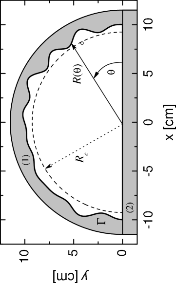
Figure 1: Sketch of the chaotic half-circular 3D microwave rough billiard in the $xy$ plane. Dimensions are given in cm. The cavity sidewalls are marked by 1 and 2 (see text). Squared wave functions $|\psi_{N,p}(R_{c},\theta)|^{2}$ were evaluated on a half-circle of fixed radius $R_{c}=9.25$ cm. Billiard’s rough boundary $\Gamma$ is marked with the bold line. The white circle centered at $x=8.12$ cm and $y=4.13$ cm marks the position of the hole drilled in the upper wall of the cavity. The hole was used to introduce the perturber inside the cavity in order to measure the $z$-component of the electric field distributions $E_{N,p}({\bf x})$.

In the experiment we used 3D cavity with the translational symmetry in the shape of a rough half-circle (Fig. 1) with the height $h=60$ mm. The cavity was made of polished aluminium. The upper and bottom walls of the cavity were attached to the sidewalls with 48 screws in order to make good electrical contact.

Assuming that the direction of the translational symmetry of the cavity is along the $z$-axis the boundary conditions at $z=0$ and $z=h$ demand that the $z$ dependence of the $z$-component of the electric and magnetic fields $E_{N,p}({\bf x})$ and $B_{N,p}({\bf x})$ of TM modes be in the form $E_{N,p}({\bf x})\equiv E_{N,p}(x,y,z)=A_{N,p}\psi_{N,p}(x,y)f_{p}(z)$, where $f_{p}(z)=\cos(p\pi z/h)$, $p=0,1,2\ldots$, $A_{N,p}$ is the normalization constant and $B_{N,p}({\bf x})=0$. The dependence of $E_{N,p}({\bf x})$ on the plane cross section coordinates we denote by the amplitude $\psi_{N,p}(x,y)\equiv E_{N,p}(x,y)$. Then, the amplitude $\psi_{N,p}(x,y)$ satisfies the Helmholtz equation

$$(\bigtriangleup_{\bot}+k_{N,p}^{2})\psi_{N,p}(x,y)=0,$$

where $\bigtriangleup_{\bot}$ is two-dimensional Laplacian operator and $k_{N,p}=(k_{N}^{2}-(p\pi/h)^{2})^{1/2}$ is the effective wave vector. The wave vector $k_{N}=2\pi\nu_{N}/c$, where $\nu_{N}$ is the resonance frequency of the level $N$ and $c$ is the speed of light in the vacuum. One can easily see that the equation (1) is equivalent to the Schrödinger equation (in units $\hbar=1$) describing a particle of mass $m=1/2$ with the kinetic energy $k_{N}^{2}$ in an external potential $V=(p\pi/h)^{2}$ Kim2005 . Therefore, 3D microwave cavities can be effectively used beyond the standard 2D frequency limit (the case $p=0$) Hans in simulation of quantum systems. The amplitude $\psi_{N,p}(x,y)$ fulfills Dirichlet boundary conditions on the sidewalls of the billiard and therefore, throughout the text it is also called the wave functions $\psi_{N}(x,y)$. It is worth noting that the full electric field $E_{N,p}({\bf x})$ satisfies Neumann boundary conditions at the top and the bottom of the cavity.

The measurements of $E_{N,p}({\bf x})$ of a 3D microwave cavity allowed us to test experimentally an important finding of the papers by Blum et al. Blum2002 and Bogomolny and Schmit Bogomolny2002 which connects the number of nodal domains of 2D billiards with the level number $N$. We will show that for the 3D cavities with the translational symmetry the number of nodal domains $\aleph_{N_{\bot}}$ lying on the cross-sectional planes of the cavity is connected with the two-dimensional level number $N_{\bot}$. The condition $E_{N,p}({\bf x})|_{z=const}=0$ on the cross-sectional planes of the cavity determines a set of nodal lines which separate regions (nodal domains) with opposite signs of the electric field distribution $E_{N,p}({\bf x})|_{z=const}$.

The value of the level number $N$ of the 3D cavity was evaluated from the Balian–Bloch formula Balian .

$$N(k)=\frac{1}{3\pi^{2}}Vk^{3}-\frac{2}{3\pi^{2}}\int_{S}\frac{d\sigma_{\omega}}{R_{\omega}}k,$$

where k is the wave vector, $V=(9.43\pm 0.01)\cdot 10^{-4}$ m³ is the volume of the cavity and $\int_{S}\frac{d\sigma_{\omega}}{R_{\omega}}=0.932$ m $\pm 0.005$ m is the surface curvature averaged over the surface of the cavity. We used this formula because of the relatively low quality factor of the cavity ($Q\simeq 4000$) some resonances overlapped.

The two-dimensional level number $N_{\bot}$ is defined by the standard Weyl–Bloch formula $N_{\bot}=\frac{A}{4\pi}k_{N,p}^{2}-\frac{P}{4\pi}k_{N,p}$, where $A=(1.572\pm 0.002)\cdot 10^{-2}$ m² and $P=0.537$ m $\pm 0.001$ m are the cross-sectional plane area of the cavity and its perimeter, respectively.

The cavity sidewalls consist of two segments (see Fig. 1). The rough segment 1 is described on the cross-sectional planes by the radius function $R(\theta)=R_{0}+\sum_{m=2}^{M}{a_{m}\sin(m\theta+\phi_{m})}$, where the mean radius $R_{0}$=10.0 cm, $M=20$, $a_{m}$ and $\phi_{m}$ are uniformly distributed on [0.084,0.091] cm and [0,2$\pi$], respectively, and $0\leq\theta<{\pi}$. (For convenience, the polar coordinates $r$ and $\theta$ are used instead of the Cartesian ones $x$ and $y$.) It is worth noting that following our earlier experience Hlushchuk01b ; Hlushchuk01 we decided to use a rough desymmetrized half-circular cavity instead of a rough circular cavity, because the first one lowers the number of nearly degenerated eigenfrequencies. Additionally, a half-circular geometry of the cavity was suitable in the procedure of accurate measurements of the electric field distributions inside the billiard.

The roughness of a billiard on the cross-sectional planes can be characterized by the function $k(\theta)=(dR/d\theta)/R_{0}$. For our microwave billiard we have the angle average $\tilde{k}=(\left<k^{2}(\theta)\right>_{\theta})^{1/2}\simeq 0.400$. The value of $\tilde{k}$ is much above the chaos border $k_{c}=M^{-5/2}=0.00056$ Frahm97 which indicates that in such a billiard the classical dynamics is diffusive in orbital momentum due to collisions with the rough boundary.

The other properties of the billiard Frahm are also determined by the roughness parameter $\tilde{k}$. The amplitudes $\psi_{N,p}(r,\theta)$ are localized for the two-dimensional level number $N_{\bot}<N_{e}=1/128\tilde{k}^{4}$. Because of a large value of the roughness parameter $\tilde{k}$ the localization border lies very low, $N_{e}\simeq 1$. The border of Breit-Wigner regime is $N_{W}=M^{2}/48\tilde{k}^{2}\simeq 52$. It means that between $N_{e}<N_{\bot}<N_{W}$ Wigner ergodicity Frahm ought to be observed and for $N_{\bot}>N_{W}$ Shnirelman ergodicity should emerge.

In order to measure the amplitudes $\psi_{N,p}(r,\theta)$ of the 3D electric field distributions we used an effective method described in Savytskyy2003 . It is based on the perturbation technique and preparation of the “trial functions”. In this method the amplitudes $\psi_{N}(r,\theta)$ (electric field distribution $E_{N}(r,\theta)$ inside the cavity) are determined from the form of electric field $E_{N,p}(R_{c},\theta)$ evaluated on a half-circle of fixed radius $R_{c}$ (see Fig. 1). The first step in evaluation of $E_{N,p}(R_{c},\theta)$ is measurement of $|E_{N,p}(R_{c},\theta)|^{2}$. The perturbation technique developed in Slater52 and used successfully in Slater52 ; Sridhar91 ; Richter00 ; Anlage98 was implemented for this purpose. In this method a small perturber is introduced inside the cavity to alter its resonant frequency.

The perturber (4.0 mm in length and 0.3 mm in diameter, oriented in $z$-direction) was moved by the stepper motor via the Kevlar line hidden in the groove (0.4 mm wide, 1.0 mm deep) made in the cavity’s bottom wall along the half-circle $R_{c}$. Before closing the cavity we carefully inspected whether the pin moves smoothly, oriented in vertical position. Using such a perturber we had no positive frequency shifts that would exceed the uncertainty of frequency shift measurements (15 kHz).

In order to determine the dependence of the electric field distributions $E_{N,p}({\bf x})$ on the $z$ coordinate and to estimate the wave vector $k_{3}=p\pi/h$ we measured the electric field inside the 3D cavity along the $z$-axis. The perturber (4.5 mm in length and 0.3 mm in diameter) was attached to the Kevlar line and moved by the stepper motor. It entered and exited the cavity by small holes (0.4 mm) drilled in the upper and the bottom walls of the cavity. The both holes were located at the position: $r=9.11$ cm, $\theta=0.47$ radians.

To eliminate the variation of resonant frequencies connected with the thermal expansion of the aluminium cavity the temperature of the cavity was stabilized with the accuracy of 0.05 $\deg$.

Using a field perturbation technique we were able to measure squared wave functions $|\psi_{N,p}(R_{c},\theta)|^{2}$ for 80 TM modes within the region $2\leq N\leq 489$. The range of corresponding eigenfrequencies was from $\nu_{2}\simeq 2.47$ GHz to $\nu_{489}\simeq 11.99$ GHz. The measurements were performed at 0.36 mm steps along a half-circle with fixed radius $R_{c}=9.25$ cm. This step was small enough to reveal in details the space structure of high-lying levels.

Figure 2: Panel (a): Squared wave function $|\psi_{430,2}(R_{c},\theta)|^{2}$ (in arbitrary units) measured on a half-circle with radius $R_{c}=9.25$ cm ($\nu_{430}\simeq 11.50$ GHz). Panel (b): Squared $z$-component of the electric field distribution $|f_{2}(z)|^{2}$ measured at $r=9.11$ cm and $\theta=0.47$ radians.

In Fig. 2 (a) and Fig. 2 (b) we show the examples of the squared amplitude $|\psi_{N,p}(R_{c},\theta)|^{2}$ and the squared $z$-component of the field, respectively, evaluated for the level number $N=430$.

The perturbation method used in our measurements allows us to extract information about the modulus of the wave function amplitude $|\psi_{N,p}(R_{c},\theta)|$ at any given point of the cross-sectional plane $z=0$ but it doesn’t allow to determine the sign of $\psi_{N,p}(R_{c},\theta)$. In order to obtain information about the sign of $\psi_{N,p}(R_{c},\theta)$ we used the method of the “trial wave function” precisely described in Savytskyy2003 ; Savytskyy2004 ; Hul2005 .

The amplitudes $\psi_{N,p}(r,\theta)$ of the electric field distributions of a rough half-circular 3D billiard may be expanded in terms of circular waves (here only odd states in expansion are considered)

$$\psi_{N,p}(r,\theta)=\sum_{s=1}^{L}a_{s}J_{s}(k_{N,p}r)\sin(s\theta),$$

where $J_{s}$ is the Bessel function of order $s$.

In Eq. (5) the number of basis functions is limited to $L=k_{N,p}r_{max}=l_{N}^{max}$, where $r_{max}=10.64$ cm is the maximum radius of the cavity. $l_{N}^{max}=k_{N,p}r_{max}$ is a semiclassical estimate for the maximum possible angular momentum for a given $k_{N}$. Circular waves with angular momentum $s>L$ correspond to evanescent waves and can be neglected. Coefficients $a_{s}$ may be extracted from the “trial wave function” $\psi_{N,p}(R_{c},\theta)$ via

$$a_{s}=[\frac{\pi}{2}J_{s}(k_{N,p}R_{c})]^{-1}\int_{0}^{\pi}\psi_{N,p}(R_{c},\theta)\sin(s\theta)d\theta.$$

Due to experimental uncertainties and the finite step size in the measurements of $|\psi_{N,p}(R_{c},\theta)|^{2}$ the wave functions $\psi_{N,p}(r,\theta)$ are not exactly zero at the boundary $\Gamma$. As the quantitative measure of the sign assignment quality we chose the integral $I=\gamma\int_{\Gamma}|\psi_{N,p}(r,\theta)|^{2}dl$ calculated along the billiard’s rough boundary $\Gamma$, where $\gamma$ is length of $\Gamma$. For correctly reconstructed wave functions the integral $I$ was several times smaller than in the case of not correctly reconstructed ones.

It is worth noting that since the pin is attached to the line it cannot be stuck. However, one may assume that during the movement the pin may be accidentally, from time to time, slightly slanted, adding small ”a noise-like component” to the measured electric field. The formula (5) shows that each wave function is expanded in terms of $L$ circular waves which filters out noise-like higher frequency Fourier components from the reconstructed wave function. The same filtering removes out the influence of the experimental uncertainties of frequency shifts on the reconstructed wave functions.

Figure 3: The “trial wave function” $\psi_{430,2}(R_{c},\theta)$ (in arbitrary units) with the correctly assigned signs, which was used in the reconstruction of the wave function $E_{430,2}(r,\theta,z)$ of the billiard (see Fig. 4).

In Fig. 3 we show the “trial wave function” $\psi_{430,2}(R_{c},\theta)$ with the correctly assigned signs, which was used in the reconstruction of the wave function $\psi_{430,2}(r,\theta)$ of the billiard (see Fig. 4). In Fig. 4 different nodal domains are separated by the bold full lines.

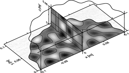
Figure 4: The reconstructed wave function $\psi_{430,2}(r,\theta)$ of the chaotic half-circular microwave rough billiard. The amplitudes have been converted into a grey scale with white corresponding to large positive and black corresponding to large negative values, respectively. The structure of the nodal lines are shown by the bold full lines. Dimensions of the billiard are given in cm. In the figure the $z$ dependence of the electric field distribution $E_{430,2}(r,\theta,z)|_{x=0}\propto\psi_{430,2}(r,\theta)|_{x=0}f_{2}(z)$ is also shown.

Using the method of the “trial wave function” we were able to reconstruct 75 experimental wave functions $\psi_{N,p}(r,\theta)$, which belonged to TM modes of the rough half-circular 3D billiard with the level number $N$ between 2 and 489. The remaining wave functions belonging to TM modes, from the range $N=2-489$, were not reconstructed because of near-degeneration of the neighboring eigenfrequencies or due to the problems with the measurements of $|\psi_{N,p}(R_{c},\theta)|^{2}$ along a half-circle coinciding for its significant part with one of the nodal lines of $\psi_{N,p}(r,\theta)$.

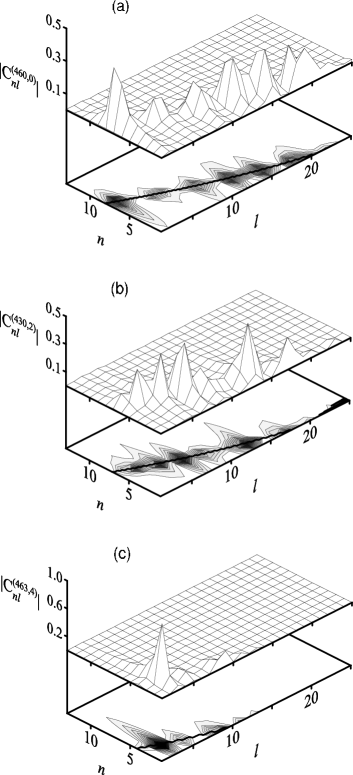
Figure 5: Structure of the energy surface of the wave functions lying close to the boarder of the regimes of Breit-Wigner and Shnirelman ergodicity ($N_{W}=52$), panels (a) and (b), and for the low wave function in the regime of Breit-Wigner ergodicity, panel (c). Panel (a): The moduli of amplitudes $|C^{(460,0)}_{nl}|$ for the wave function $\psi_{460,0}(r,\theta)$, $N_{\bot}=65$, lying in the regime of Shnirelman ergodicity. Panel (b): The moduli of amplitudes $|C^{(430,2)}_{nl}|$ for the wave function $\psi_{430,2}(r,\theta)$, $N_{\bot}=50$, in the regime of Breit-Wigner ergodicity . Panel (c): The moduli of amplitudes $|C^{(463,4)}_{nl}|$ for the wave function $\psi_{463,4}(r,\theta)$ lying in the regime of Breit-Wigner ergodicity close to the localization boarder. Full lines show the semiclassical estimation of the energy surface (see text).

The borders of Breit-Wigner and Shnirelman ergodicities are not sharp. Therefore, to check ergodicity of the billiard’s wave functions $\psi_{N,p}(r,\theta)$, especially close to the borders, one should use some additional measures such as e.g., calculation of the structures of their energy surfaces Frahm97 . For this reason we extracted wave function amplitudes $C^{(N,p)}_{nl}=\left<n,l|N,p\right>$ in the basis $n,l$ of a half-circular billiard with radius $r_{max}$, where $n=1,2,3\ldots$ enumerates the zeros of the Bessel functions and $l=1,2,3\ldots$ is the angular quantum number. The moduli of amplitudes $|C^{(N,p)}_{nl}|$ and their projections into the energy surface for the experimental wave functions $\psi_{460,0}(r,\theta)$, $\psi_{430,2}(r,\theta)$ and $\psi_{463,4}(r,\theta)$ are shown in Fig. 5(a-c). As expected, on the border of the regimes of Breit-Wigner and Shnirelman ergodicity the wave functions $\psi_{460,0}(r,\theta)$ ($N_{\bot}=65$) and $\psi_{430,2}(r,\theta)$ ($N_{\bot}=50$) are extended homogeneously over the whole energy surface Hlushchuk01 . The wave function $\psi_{463,4}(r,\theta)$, $N_{\bot}=16$, which lies closer to the localization boarder, is also extended along the energy surface, however it displays the tendency to localization in $n,l$ basis (see Fig. 5(c)). The full lines on the projection planes in Fig. 5(a-c) mark the energy surface of a half-circular billiard $H(n,l)=k^{2}_{N,p}$ estimated from the semiclassical formula Hlushchuk01b : $\sqrt{(l^{max}_{N})^{2}-l^{2}}-l\arctan(l^{-1}\sqrt{(l^{max}_{N})^{2}-l^{2}})+\pi/4=\pi n$. It is clearly visible that the peaks $|C^{(N,p)}_{nl}|$ are spread almost perfectly along the lines marking the energy surface.

Figure 6: The number of nodal domains $\aleph_{N_{\bot}}$ (full circles) on the cross-section planes of the chaotic half-circular 3D microwave rough billiard. Full line shows the least squares fit $\aleph_{N_{\bot}}=a_{1}N_{\bot}+b_{1}\sqrt{N_{\bot}}$ to the experimental data (see text), where $a_{1}=0.059\pm 0.029$, $b_{1}=0.991\pm 0.190$. The prediction of the theory of Bogomolny and Schmit Bogomolny2002 $a_{1}=0.062$.

The number of nodal domains $\aleph_{N_{\bot}}$ on the cross-sectional plane $z=0$ vs. the level number $N_{\bot}$ in the chaotic 3D microwave rough billiard is plotted in Fig. 6. The full line in Fig. 6 shows the least squares fit $\aleph_{N_{\bot}}=a_{1}N_{\bot}+b_{1}\sqrt{N_{\bot}}$ of the experimental data, where $a_{1}=0.059\pm 0.029$, $b_{1}=0.991\pm 0.190$. The coefficient $a_{1}=0.059\pm 0.029$ coincides with the prediction of the percolation model of Bogomolny and Schmit Bogomolny2002 $\aleph_{N_{\bot}}/N_{\bot}\simeq 0.062$ within the error limits. The relatively large uncertainty of the coefficient $a_{1}$ is connected with the fact that in the least squares fit procedure we used only 27 higher states with $N_{\bot}>20$. The states with lower $N_{\bot}$ were not taken into account because they were not fully chaotic (see Fig. 5(c)). The second term in the least squares fit corresponds to a contribution of boundary domains, i.e. domains, which include the billiard boundary. Numerical calculations of Blum et al. Blum2002 performed for the Sinai and stadium billiards showed that the number of boundary domains scales as the number of the boundary intersections, that is as $\sqrt{N_{\bot}}$. Our results clearly suggest that in the rough billiard, at the level numbers $20<N_{\bot}\leq 65$, the boundary domains also significantly influence the scaling of the number of nodal domains $\aleph_{N_{\bot}}$, leading to the departure from the predicted scaling $\aleph_{N_{\bot}}\sim N_{\bot}$.

In summary, we measured the wave functions of the chaotic 3D rough microwave billiard with the translational symmetry up to the level number $N=489$. We showed that for the two-dimensional level numbers $20<N_{\bot}\leq 65$ the scaling of the number of nodal domains $\aleph_{N_{\bot}}$ significantly departures from the predicted scaling $\aleph_{N_{\bot}}\sim N_{\bot}$, which suggests that the boundary domains influence the scaling Bogomolny2002 . In the limit $N_{\bot}\rightarrow\infty$ the least squares fit of the experimental data yields the asymptotic number of nodal domains $\aleph_{N_{\bot}}/N_{\bot}\simeq a_{1}=0.059\pm 0.029$ that is close to the theoretical prediction $\aleph_{N_{\bot}}/N_{\bot}\simeq 0.062$. Finally, our results show that 3D microwave cavities with the translational symmetry can be effectively used beyond the standard 2D frequency limit in simulation of quantum systems.

Acknowledgments. This work was partially supported by the Ministry of Education and Science grant No. N202 099 31/0746.

References

- (1) G. Blum, S. Gnutzmann, and U. Smilansky, Phys. Rev. Lett. 88, 114101-1 (2002).
- (2) E. Bogomolny and C. Schmit, Phys. Rev. Lett. 88, 114102-1 (2002).
- (3) N. Savytskyy, O. Hul, and L. Sirko, Phys. Rev. E 70, 056209 (2004).
- (4) O. Hul, N. Savytskyy, O. Tymoshchuk, S. Bauch, and L. Sirko, Phys. Rev. E 72, 066212 (2005).
- (5) O. Hul, N. Savytskyy, O. Tymoshchuk, S. Bauch, and L. Sirko, Acta Phys. Pol. A 109, 73 (2006).
- (6) S. Deus, P.M. Koch, and L. Sirko, Phys. Rev. E 52, 1146 (1995).
- (7) H. Alt, C. Dembowski, H.-D. Gräf, R. Hofferbert, H. Rehfeld, A. Richter, R. Schuhmann, and T. Weinland, Phys. Rev. Lett. 79,1026 (1997).
- (8) U. Dörr, H.-J. Stöckmann, M. Barth, and U. Kuhl, Phys. Rev. Lett. 80, 1030 (1998).
- (9) B. Eckhardt, U. Dörr, U. Kuhl, and H.-J. Stöckmann, Europhys. Lett. 46, 134 (1999).
- (10) C. Dembowski, B. Dietz, H.-D. Gräf, A. Heine, T. Papenbrock, A. Richter, and C. Richter, Phys. Rev. Lett. 89, 064101 (2002).
- (11) O. Tymoshchuk, N. Savytskyy, O. Hul, S. Bauch, and L. Sirko, Phys. Rev. E accepted for publication (2007).
- (12) H. Primack and U. Smilansky, Phys. Rev. Lett. 74, 4831 (1995).
- (13) T. Prosen, Phys. Lett. A 233, 323 (1997).
- (14) L. R. Arnaut, Phys. Rev. E 73, 036604 (2006).
- (15) Y.-H. Kim, U. Kuhl, H.-J. Stöckmann, and J. P. Bird, J. Phys.: Condens. Matter 17, L191 (2005).
- (16) H.-J. Stöckmann, J. Stein, Phys. Rev. Lett. 64, 2215 (1990).
- (17) R. Balian and C. Bloch, Ann. Phys. (N.Y.) 84, 559 (1974); Ann. Phys. (N.Y.) 64, 271(E) (1971).
- (18) Y. Hlushchuk, A. Błȩdowski, N. Savytskyy, and L. Sirko, Physica Scripta 64, 192 (2001).
- (19) Y. Hlushchuk, L. Sirko, U. Kuhl, M. Barth, H.-J. Stöckmann, Phys. Rev. E 63, 046208-1 (2001).
- (20) K.M. Frahm and D.L. Shepelyansky, Phys. Rev. Lett. 78, 1440 (1997).
- (21) K.M. Frahm and D.L. Shepelyansky, Phys. Rev. Lett. 79, 1833 (1997).
- (22) N. Savytskyy and L. Sirko, Phys. Rev. E 65, 066202-1 (2002).
- (23) L.C. Maier and J.C. Slater, J. Appl. Phys. 23, 68 (1952).
- (24) S. Sridhar, Phys. Rev. Lett. 67, 785 (1991).
- (25) C. Dembowski, H.-D. Gräf, A. Heine, R. Hofferbert, H. Rehfeld, and A. Richter, Phys. Rev. Lett. 84, 867 (2000).
- (26) D.H. Wu, J.S.A. Bridgewater, A. Gokirmak, and S.M. Anlage, Phys. Rev. Lett. 81, 2890 (1998).