Beam Polarization at the ILC: the Physics Impact and the Accelerator Solutions

Abstract

In this contribution accelerator solutions for polarized beams and their impact on physics measurements are discussed. Focus are physics requirements for precision polarimetry near the interaction point and their realization with polarized sources. Based on the ILC baseline programme as described in the Reference Design Report (RDR), recent developments are discussed and evaluated taking into account physics runs at beam energies between 100 GeV and 250 GeV, as well as calibration runs on the Z-pole and options as the 1 TeV upgrade and GigaZ.

1 Introduction

With the start of LHC operation the physics frontier will be opened to very high energies. The full understanding of the results requires completion by precision measurements with a lepton collider. Due to parity violation in weak interactions polarized beams are essential to unravel new phenomena and will play a crucial role in that programme.

The beam polarization and its importance for physics at an e⁺e^- collider has been discussed in details over years. A comprehensive overview on the physics prospectives with polarized beams can be found in reference [2]. The focus of this contribution is beam polarization and its precise measurement. As precision luminosity and energy measurement, the performance of polarimeters has to be implicated in the the machine design from the beginning to achieve the physics goals for a future lepton collider as the ILC. The baseline configuration for the ILC is described in the Reference Design Report (RDR) [3]. The electron beam will be highly polarized: based on the experience of SLAC, at least 80% polarization are expected. The polarization near the collision will be measured with Compton polarimeters positioned upstream and downstream the interaction point (IP). The complementarity of these two polarimeters as well as the flexibility of the suggested solutions for various ILC energies will be discussed in section 4.

In compliance with the RDR [3], the positron source configuration of the ILC is based on the helical undulator and provides a polarized positron beam. The degree of positron beam polarization is smaller than planned for the upgrade, about 30% – 45%, but sufficient to be used for physics measurements.

In order to preserve the polarization, the spin vectors have to be aligned parallel to the rotation axis of the damping ring. Hence, in the electron and positron line spin rotator systems [4] rotate the spin vector from the longitudinal to the vertical direction before the Damping Ring (DR) and back after. However, there is one decisive feature: the helicity of the electrons can be chosen on a train-by-train basis by switching the laser polarization. The helicity of positrons is defined by the orientation of the helix winding in the undulator and additional instrumentation is needed to provide fast helicity reversal also for positrons. The fact that this instrumentation is not yet included in the baseline design initiated discussions whether fast helicity reversal would be really needed taking into account also the costs. The consequences of fast or slow helicity reversal will be pointed out in in section 2.

Recently the high precision polarization measurement near the IP has been compromised by proposals to combine machine instrumentation and protection equipment with the polarimeter chicane. The impact of such design on polarimetry has been discussed at this and previous workshops, details can be found in references [5, 6]. Here in this contribution, the basic polarimeter design required for appropriate and reliable ILC polarization measurements will be emphasized.

2 The Precision Requirements

The strong potential of the ILC is the precision: Standard Model processes as fermion pair production, W⁺W^- and also the Higgs production, will be obtained with high statistics and allow uncertainties at the per-mille level. This demands measurements of energy and luminosity with high stability and with precision at a level ${\cal O}(10^{-4})$ as mentioned in the physics part of the RDR [7]. The challenge of polarization becomes clear by comparing uncertainties in statistics, luminosity and energy with the precision that can be achieved for polarization measurements:

$$\frac{\Delta\sigma}{\sigma}\propto\frac{1}{\sqrt{N}}\oplus\frac{\Delta{\cal{L}}}{{\cal{L}}}\oplus\frac{\Delta E}{E}\oplus\frac{\Delta P}{P}\,.$$ (1)

Studies also presented at this workshop [8] show that a precision of $\Delta P/P\approx 0.25\%$ is possible (see also section 4).

There are three methods to measure polarization of colliding beams: upstream and downstream of the IP, as well as using annihilation events.

2.1 Basic Remarks

In general, the cross section for s-channel processes can be written as

$$\sigma_{\pm\pm} = \frac{1}{4}\sigma_{0}\left[1-|P_{e^{+}}||P_{e^{-}}|+A_{\mathrm{LR}}\left(\mp|P_{e^{+}}|\pm|P_{e^{-}}|\right)\right]$$ (2)

$$\sigma_{\mp\pm} = \frac{1}{4}\sigma_{0}\left[1+|P_{e^{+}}||P_{e^{-}}|+A_{\mathrm{LR}}\left(\pm|P_{e^{+}}|\pm|P_{e^{-}}|\right)\right]$$ (3)

where ‘$+~{}-$’, ‘$-~{}-$’, ‘$-~{}+$’ and ‘$+~{}+$’ are the different combinations of helicities in the initial state, $A_{\mathrm{LR}}$ the Left-Right asymmetry and $\sigma_{0}$ the unpolarized cross section. In the Standard Model, the cross sections $\sigma_{\pm\pm}$ are zero for 100% polarized beams. The asymmetry, $A_{\mathrm{LR}}$, can be determined from the measured left-right asymmetric cross sections with

$$A_{\mathrm{LR}}=\frac{\sigma_{-+}-\sigma_{+-}}{\sigma_{-+}+\sigma_{+-}}\cdot\frac{1-P_{e^{+}}P_{e^{-}}}{P_{e^{+}}-P_{e^{-}}}=\frac{A_{\mathrm{LR}}^{meas}}{P_{eff}}\,,$$ (4)

and the unpolarized cross section is

$$\sigma_{0}=\frac{1}{2}\cdot\frac{\sigma_{-+}+\sigma_{+-}}{1-P_{e^{+}}P_{e^{-}}}\,.$$ (5)

In case of electron polarization only, these observables simplify to

$$\sigma_{\mp}=\sigma_{0}\left[1\pm{\mathcal{P}}_{e^{-}}\,A_{\mathrm{LR}}\right]\,,~{}~{}~{}~{}~{}~{}~{}A_{\mathrm{LR}}=\frac{\sigma_{-}-\sigma_{+}}{\sigma_{-}+\sigma_{+}}\cdot\frac{1}{P_{e^{-}}}=\frac{A_{\mathrm{LR}}^{meas}}{P_{e}}$$ (6)

The event numbers, $N_{\mp\pm}$ and $N_{\pm\pm}$ are measured if the luminosities ${\cal{L}}_{\mp\pm}$, ${\cal{L}}_{\pm\pm}$, are delivered to the different initial states with the polarizations $(\mp|P_{e^{-}}|,\pm|P_{e^{+}}|)$ and $(\pm|P_{e^{-}}|,\pm|P_{e^{+}}|)$. If the luminosity is equally distributed to the ’$-~{}+$’ and ’$+~{}-$’ initial states, ${\cal{L}}_{\mp\pm}={\cal{L}}_{\pm\mp}$, the Left-Right asymmetry is

$$A_{\mathrm{LR}}=\frac{N_{-+}-N_{+-}}{N_{-+}+N_{+-}}\cdot\frac{1}{P_{eff}}\,.$$ (7)

From equations (4) – (7) one infers that only the luminosity-weighted averaged polarization matters. Neglecting the uncertainties of energy and luminosity, the error on $A_{\mathrm{LR}}$ is

$$\Delta A_{\mathrm{LR}}=\sqrt{\frac{1-P^{2}\cdot A_{\mathrm{LR}}^{2}}{NP}+{A_{\mathrm{LR}}^{2}}\frac{(\Delta P)^{2}}{P^{2}}}\,,$$ (8)

where $P$ is either $P_{eff}$ if both beams are polarized or $P_{e^{-}}$ in case of electron polarization only. For high statistics $\Delta A_{\mathrm{LR}}$ is dominated by the uncertainty of the polarization measurement.

Because of error propagation the uncertainty of the effective polarization, $\Delta{\mathcal{P}}_{\rm{eff}}/{\mathcal{P}}_{\rm{eff}}$, is considerably smaller than the uncertainty of the individual polarizations $P_{e^{+}}$ and $P_{e^{-}}$. In addition, with polarized e⁺ and e^- the luminosity is effectively increased by a factor $1+|P_{e^{+}}P_{e^{-}}|$. This great advantage can be utilized for measurements if the luminosity-weighted polarizations are equally distributed only to ’opposite’ initial states, i.e. ’$+$ $-$’ and ’$-$ $+$’. Otherwise, corrections and error propagation would lead to larger errors, and systematic uncertainties, in particular time-dependent uncertainties, do not cancel. The individual polarizations, $P_{e^{-}}$ and $P_{e^{+}}$ occur linearly and bi-linearly in equations (2) and (3). That complicates even tiny corrections substantially and requires also the knowledge of correlations between $P_{e^{-}}$ and $P_{e^{+}}$.

All these facts emphasize the importance of high precision polarization measurement including high time resolution and cross checks.

3 Polarized Sources

3.1 Polarized Electron Source

Polarized electrons are produced from a DC photo-cathode gun. With fast Pockels cells the circular polarization of the source laser beam is set and can be reversed train-to-train, thereby allowing fast reversals of the electron spin. A Mott polarimeter located in a diagnostic line will be used to determine the electron polarization near the source. Normal-conducting structures are used for bunching and pre-acceleration to 76 MeV, afterward the beam is accelerated to 5 GeV in a superconducting linac. Before injection into the damping ring the spin is rotated to the vertical with superconducting solenoids, the rotation back to the longitudinal is performed before injection to the main linac. A separate superconducting structure is used for bunch compression. The sketch of the electron source as given in the RDR is shown in Figure 1.

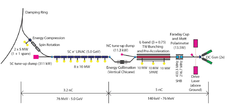
Figure 1: Sketch of the electron source as given in the RDR.

Spin rotation at the source could be done also at lower energies as proposed in reference [9]. The requirements for the solenoid are less stringent for spin rotation at 1.7 GeV; detailed studies how such system could be implemented have still to be done. Spin rotation near the gun using a Wien filter is not recommended since substantial emittance growth is expected [10].

Concerning polarization, charge and lifetime, the SLC polarized electron source meets the ILC requirements. But the long bunch trains need a special laser system and normal conducting RF structures that can handle the high RF power. Both requirements are considered as manageable.

3.2 Polarized Positron Source

The positron source uses photo-production to generate positrons [3]. The electron main linac beam passes through a long helical undulator to generate a multi-MeV photon beam, which then strikes a thin metal target to generate positrons in an electromagnetic shower. The positrons are captured, accelerated, separated from the shower constituents and unused photon beam and then are transported to the Damping Ring. Although the baseline design only requires unpolarized positrons, the positron beam produced using a helical undulator has a polarization of ${\mathcal{P}}_{e^{+}}\apprge 30\,$%. Simulation studies show that bunch (energy) compression would increase the positron capture efficiency at the source, with which the positron polarization could even reach ${\mathcal{P}}_{e^{+}}\apprge 45\,$% at the beginning of the ILC physics program. [11]. Beamline space has been reserved for an upgrade to 60% polarization. A sketch of the ILC positron source as described in the RDR is presented in Figure 2.

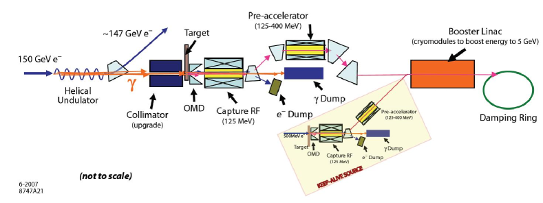
Figure 2: Sketch of the positron source as given in the RDR.

Low energy polarimetry for the positron beam is not foreseen in the RDR. Different methods and positions for a polarimeter have been studied [12] based on the special parameters of the positron beam at the source, in particular the relative large transverse beam size. Directly after the capture section (125 MeV) a Compton transmission polarimeter can be used, after pre-acceleration at 400 MeV a Bhabha polarimeter and after the damping, at 5 GeV before the main linac, a Compton polarimeter is recommended to measure the positron beam polarization.

3.2.1 Spin Rotation at the Positron Source

There are two ways to use the positron beam:

1. Physics measurements with a positron polarization of about ${\mathcal{P}}_{e^{+}}\apprge 30-45\,$%.

2. Unpolarized positrons at the $e^{+}e^{-}$–IP.

In the first case (1), the polarized positron beam is transported to the $e^{+}e^{-}$–IP with minimal spin diffusion and the degree of polarization is measured with high precision of 0.25% near the interaction region with upstream and downstream polarimeters (see next sections). Spin rotator systems are described in the RDR and are included in the positron beam transport lines from the Linac to the Damping Ring (LTR) and from the Damping Ring to the Linac (RTL). The polarized positrons collide with polarized electrons whose helicity is reversed very frequently (train-by-train). Following the discussion in section 2.1, it must be possible to flip the positron helicity with the same rate. In the current baseline design, however, the positron helicity can only be slowly reversed by changing the polarity of the superconducting spin rotator magnets. As a consequence, the luminosities and the luminosity weighted polarizations are different for the measurements, systematic uncertainties do not cancel and finally the required precision cannot be reached. With a positron helicity reversal less frequent than for electrons half of the running time will be spent on the inefficient helicity combinations ’$+~{}+$’ and ’$-~{}-$’, any gain for the effective luminosity due to positron polarization is lost.

Hence it is strongly recommended to modify the baseline configuration to provide random selection of the positron helicity train-by-train by implementing parallel spin rotator beamlines and kicker systems in the positron Linac-to-Ring system (LTR) (see also references [6, 13]). Positron spin rotation and flipping could be done at 5 GeV [14] using superconducting solenoids or at 400 MeV [9].

As for the electron source, at 5 GeV superconducting solenoids are necessary to rotate the spin from the transverse horizontal to the vertical direction, at 400 MeV the solenoid magnets can be normal conducting and they can be smaller, demanding less tunnel space. These modifications would simplify the engineering for these systems, and reduce the costs. But in both cases, at 400 MeV and at 5 GeV, two rotation lines are needed for two opposite vertical spin directions. A fast kicker distributes the positron trains to the different lines.

In the second case (2), the 30-45% positron polarization are not delivered from the source to the experiment. The spin rotation lines are not needed in the positron line but a special scheme after the positron damping ring needs to be devised to completely destroy the positron polarization in order not to adversely effect the physics measurements. Spin tracking studies [15] have shown that the horizontal projections of the spin vectors of an $e^{+}$ or $e^{-}$ bunch do not fully decohere in the damping ring, even after 8000 turns. The zero positron polarization also needs to be measured with high precision. Further studies are needed to ensure a left-over positron DC polarization of about 0.1% will not affect physics measurements, which could result in the need for an even higher precision in this case.

In both cases, (1) and (2), it is required to measure the positron polarization with high precision, the replacement of the spin rotation and flip facility by a device to destroy the polarization to save costs is not recommended regarding the physics physics potential with polarized positrons.

4 Polarimetry near the Interaction Point

The ILC offers three methods to measure polarization after acceleration: upstream and downstream of the IP, as well as using annihilation events. Compton polarimeters are used upstream and downstream. The working principle Compton polarimeters can be found for example in reference [16]. The longitudinally polarized electron (positron) beam is hit almost head-on by a circularly polarized laser. The energy spectra of the scattered particles depend on the product of polarizations of laser and lepton beam. The measured asymmetry resulting from polarization reversal is proportional to the beam polarization.

The two polarimeters are highly complementary. The upstream polarimeter has a much higher counting rate and time granularity which is important for correlation measurements. The downstream polarimeter has access to the depolarization in the interaction. The polarimeters provide corrections and measure the polarization on short scales. Without collisions the two polarimeters can calibrate each other.

With the small errors envisaged at the ILC, it is indispensable for the final polarization measurement at the ILC to have upstream and downstream polarimetry and to get an absolute calibration from annihilation data. Cross check of the different ways to measure polarization is mandatory; this has also been confirmed by the polarimetry experience at SLC and by the beam-energy measurements at both, LEP and SLC.

To keep the corrections and systematic uncertainties small, i.e. every effort should be made to flip the helicity of electrons and positrons frequently, if possible train by train.

4.1 The Upstream Polarimeter

The upstream polarimeter is located at the beginning of the Beam Delivery System (BDS), upstream of the tuneup dump and at a distance of roughly 1.8 km to the $e^{+}e^{-}$–IP. In this position it benefits from clean beam conditions and very low backgrounds compared to any location downstream of the IP. It is therefore suited to provide very fast and precise polarization measurements before collisions.

A complete conceptual layout for the upstream polarimeter had already been worked out for TESLA in 2001 [16]. However, for the ILC, a dedicated chicane-based spectrometer was adopted for upstream polarimetry in 2005, as this configuration allows the usage of a single laser wavelength at all beam energies when the spectrometer is operated with a fixed magnetic field. The Compton edge at the detector surface is the same for all beam energies providing a homogeneous detector acceptance and equal performance for all center-of-mass energies. The layout and principle of the upstream polarimeter chicane is shown in Figure 3: the Compton IP moves laterally with the beam energy; laser, vacuum chamber and detector have to be designed accordingly.

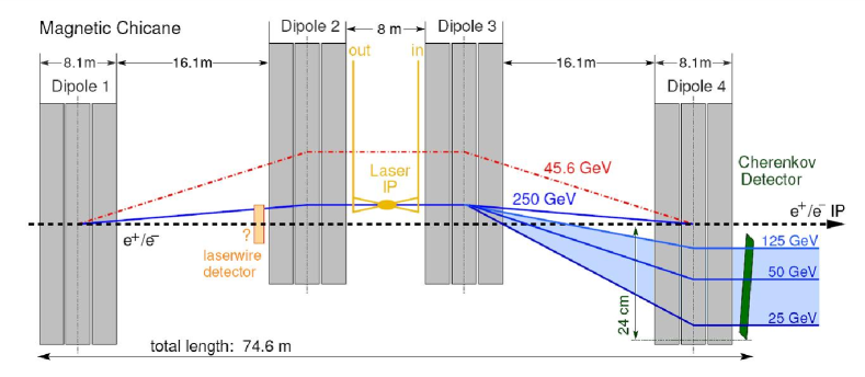
Figure 3: Sketch of the upstream polarimeter.

In this original design with a dedicated fixed-field chicane, the upstream polarimeter promised to be a superb and robust instrument with broad spectral coverage, very low background, excellent statistical performance for all machine bunches, and a high degree of redundancy.

If equipped with a suitable laser, for example a similar one as used at the FLASH source, it can include every single bunch in the measurement. This will permit virtually instant recognition of variations within each bunch train as well as time dependent effects that vary train-by-train. The statistical precision of the polarization measurement will be already 3% for any two bunches with opposite helicity, which leads to an average precision of 1% for each bunch position in the train after the passage of only 20 trains (4 seconds). The average over two entire trains with opposite helicity will have a statistical error of $\Delta\mathcal{P}/\mathcal{P}=0.1$%.

The statistical power of the upstream polarimeter depends almost exclusively on the employed laser and therefore to first order factorizes from other design aspects. However the crucial issue which drives the design of the whole polarimeter is to reach an unprecedented low systematic uncertainty of $\delta P/P\leq 0.25\%$ or better [17] with the largest uncertainties coming from the analyzing power calibration (0.2%) and the detector linearity (0.1%).

To obtain a useful polarization measurement the beam trajectories are required to be aligned to less than 50 $\mu$rad at the upstream Compton-IP, the collider-IP, and the downstream Compton-IP. This should be achievable by the beam delivery system (BDS) alignment as described in the RDR.

However, the impact of magnets in the interaction region and the crossing angle on the spin alignment needs to be addressed more thoroughly. In the extraction line, corrector magnets are needed to successfully compensate possible deflections resulting from misaligned beam and detector solenoid axes.

In an effort to reduce the cost of the long and expensive BDS system, the BDS management decided in autumn 2006 to combine the upstream polarimeter chicane with other diagnostic and machine functions (machine protection system). With the machine protection system (MPS) energy collimator in the polarimeter chicane the upstream polarimeter has to be operated with ’scaled magnetic field’ , the excellent polarimeter performance over the wide ILC energy range is lost. Another suggestion is laser wire emittance diagnostics with a detector in front of the second dipole triplet of the polarimeter chicane as can be seen also in Figure 3. It is expected that this detector creates huge background unacceptable for polarimetry. The consequences of combining the upstream polarimeter chicane with other diagnostic and machine functions were discussed at the Workshop on Polarization and Energy Measurement in April in Zeuthen [6] and at this workshop [5]. Better solutions will be found.

4.2 The Downstream Polarimeter

The downstream polarimeter is located about 150 m downstream of the $e^{+}e^{-}$–IP in the extraction line and on axis with the IP and IR magnets. It can measure the beam polarization both with and without collisions, thereby testing the calculated depolarization correction which is expected to be at the 0.1-0.2% level. A complete conceptual layout for the downstream polarimeter exists, including magnets, laser system and detector configuration.

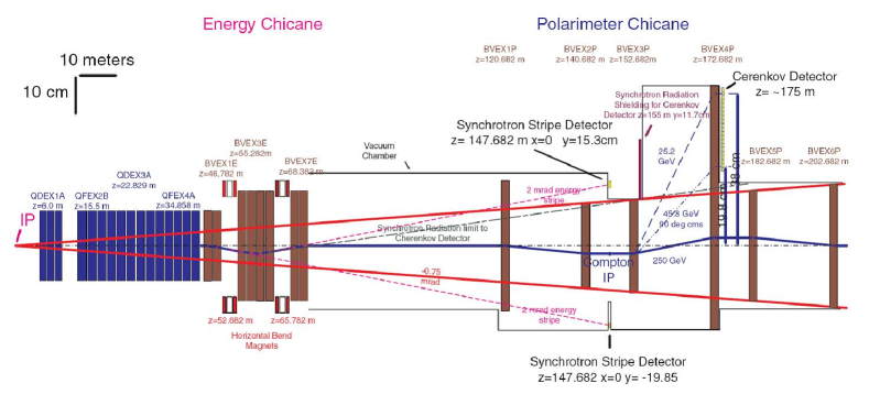
Figure 4: Sketch of the downstream polarimeter.

Figure 4 presents the sketch of the extraction line polarimeter as shown in the RDR. The downstream polarimeter needs a six-magnet chicane [18]; the additional two magnets after the Compton detector allow to operate the third and fourth magnets at higher field to deflect the Compton electrons further from the beam line and to return the beam to the nominal trajectory.

Three 10 Hz laser systems can achieve Compton collisions for three out of 2800 bunches in a train. Each laser will sample one particular bunch in a train for a time interval of a few seconds to a minute, then select a new bunch for the next time interval, and so on in a pre-determined pattern. The Compton statistics are high with about 300 Compton scattered electrons per bunch in a detector channel at the Compton edge.

With this design, a statistical uncertainty of less than 1% per minute can be achieved for each of the measured bunches. This is dominated by fluctuations in Compton luminosity due to beam jitter and laser targeting jitter and to possible background fluctuations. The statistical error due to Compton statistics in one minute, for a bunch sampled by one laser, is 0.3%. However, if compared to the average precision of the upstream polarimeter, a similar precision for each bunch position in a train could only be reached after about 17 hours.

Background studies have been carried out for disrupted beam losses and for the influence of synchrotron radiation. There are no significant beam losses for the nominal ILC parameter set and beam losses look acceptable even for the low power option. A synchrotron radiation collimator protects the Compton detector and no significant synchrotron radiation backgrounds are expected. The systematic precision is expected to be about 0.25%, with the largest uncertainties coming from the analyzing power calibration (0.2%) and detector linearity (0.1%).

In addition, it is desired to correlate the downstream polarimeter measurements with beam position measurements (BPM) at the $e^{+}e^{-}$–IP [19] by providing information from the BPM system to the polarimeter DAQ including bunch number identification.

4.3 Depolarization at the IP

For high precision measurements depolarization effects in the machine have to be known. Depolarization occurs during bunch crossing because of beam-beam effects or could be caused by misalignment, i.e. ground motion induced misalignment. Depolarization effects and their impact on physics have to be understood with high precision, for details see reference [20].

With the downstream polarimeter depolarization effects can be measured by comparing measurements with colliding and non-colliding beams and simulations. The disrupted beam is propagated down the the extraction line to simulate the the polarization measurement with the downstream polarimeter.

Current studies using Guinea Pig++ [21] and CAIN [22] show good agreement. For a nominal case in which both beams are initially assumed to be 100% longitudinally polarized, the luminosity-weighted polarization of each beam is predicted to be reduced by $0.21\%\pm 0.01\%$ compared to the initial polarization. For details see references [23, 24].

4.4 Polarimetry with Annihilation Data

Apart from the polarimeters, polarization can also be measured using annihilation data [25]. If both beams are polarized this can be done measuring the fermion-pair cross section for different helicity combinations in the initial state (Blondel scheme). If only the electron beam is polarized, W-pair production can be used to determine electron polarization with the assumption that the $e\nu W$-coupling is purely left-handed which is well tested.

4.4.1 Blondel Scheme

The annihilation method using fermion pairs is based on equations (4). By measuring all four cross sections, $\sigma_{\pm\mp}$ and $\sigma_{\pm\pm}$, a direct and independent measurements of the luminosity weighted electron and positron polarization as well as the asymmetry $A_{\mathrm{LR}}$ are possible. Nevertheless, the polarimeters near the IP are needed to monitor time dependent fluctuations in the polarizations. This Blondel-scheme is especially efficient at the Z resonance where a high rate of annihilation data is available and the polarization has to be measured with extremely high precision. At the Z peak, only a small fraction of the luminosity ($\sim 10$%) has to be delivered to the ’inefficient’ helicity combinations ’$\pm~{}\pm$’ but half of the luminosity at high energies [25].

Only a small fraction of the luminosity ($\sim 10$%) has to be delivered to the ’inefficient’ helicity combinations ’$\pm~{}\pm$’. At high energies half of the luminosity should be deliverd to the helicity combinations ’$\pm~{}\pm$’ to reach the required uncertainties for the polarization measurement. Due to the low event rates the polarization measurement with the Blondel Scheme is slow but it is a good cross check for the measurement with polarimeters. A detailed discussion of the Blondel scheme can be found in reference [26].

4.4.2 $Z$-pole Calibration Data

The GigaZ option – ILC precision measurements at the $Z$-pole – is foreseen as a running mode at a later time of ILC operation. However, calibration will require runs at the Z peak. Measurements during these runs are far beyond the statistics of GigaZ but will exceed that of LEP and provide complementary information to the presently known precision measurement of the weak mixing angle $\sin\theta_{eff}$.

Hence the precise measurements of energy and polarization at the $Z$-pole are important and should be included in the ILC baseline documents for the following reasons:

• Polarimeter calibration and cross-check against physics based polarization measurements using the Blondel scheme;

• Data from these calibration runs can also provide significant statistics for physics measurements complementary to LEP and SLC results.

Reference [27] summarizes the physics prospects with $Z$-pole calibration data.

4.4.3 Polarization Measurement with W⁺W^- Data

Also the W⁺W^- data can be used for polarization measurement [25]. The forward peak is entirely dominated by t-channel neutrino exchange and not influenced by possibly unknown triple gauge interactions. Providing long measuring times (months!) a precision of 0.1% can be reached. Nevertheless, the polarimeters are needed to correct for time-dependent relative polarization fluctuations.

5 Upgrade to $\sqrt{s}=1$ TeV

Depending on the LHC physics results an energy upgrade to 1 TeV center-of-mass will be the next step after the completion of the baseline programme. The requirements for polarimetry are the same as for $E_{cms}=500\,$GeV. The upstream polarimeter with the fixed field operation allows for precise polarization measurements at 1 TeV. This performance should not be compromised in any way. In particular, the relatively easy upgrade to operate polarimeters at beam energies above 250 GeV should not be rendered impossible by installed beam diagnostic or other instrumentation in the chicane.

6 Recommendations form the EP Workshop in Zeuthen, April 2008

At the “Workshop on Energy and Polarization Measurement” in April 2009 at DESY Zeuthen seven recommendations emerged requiring follow-up from the GDE and the Research Director (see also reference [6]). All these items were also discussed at LCWS08/ILC08.

1. Separate the functions of the upstream polarimeter chicane. Do not include an MPS energy collimator or laser-wire emittance diagnostics; use instead a separate setup for these two.

2. Modify the extraction line polarimeter chicane from a 4-magnet chicane to a 6-magnet chicane to allow the Compton electrons to be deflected further from the disrupted beam line.

3. Include precise polarization and beam energy measurements for $Z$-pole calibration runs into the baseline configuration.

4. Keep the initial positron polarization of 30-45% for physics (baseline).

5. Implement parallel spin rotator beamlines with a kicker system before the damping ring to provide rapid helicity flipping of the positron spin.

6. Move the pre-DR positron spin rotator system from 5 GeV to 400 MeV. This eliminates expensive superconducting magnets and reduces costs.

7. Move the pre-DR electron spin rotator system to the source area. This eliminates expensive superconducting magnets and reduces costs.

7 Summary

The studies, talks and discussions presented at this conference demonstrated that beam polarization and its measurement are crucial for the physics success of any future linear collider. To achieve the required precision it is absolutely decisive to employ multiple devices for testing and controlling the systematic uncertainties of each polarimeter. The polarimetry methods for the ILC are complementary: with the upstream polarimeter the measurements are performed in a clean environment, they are fast and allow to monitor time-dependent variations of polarization. The polarimeter downstream the IP will measure the disrupted beam resulting in high background and much lower statistics, but it allows access to the depolarization at the IP. Cross checks between the polarimeter results give redundancy and inter-calibration which is essential for high precision measurements. Current plans and issues for polarimeters and also energy spectrometers in the Beam Delivery System of the ILC are summarized in reference [28].

The ILC baseline design allows already from the beginning the operation with polarized electrons and polarized positrons provided the spin rotation and the fast helicity reversal for positrons will be implemented. A reversal of the positron helicity significantly slower than that of electrons is not recommended to not compromise the precision and hence the success of the ILC.

Recently to use calibration data at the Z resonance for physics has been discussed. It looks promising but further studies are needed to evaluate and to optimize these measurements.

Finally it should be remarked: many studies on different physics processes and scenarios at a future linear collider are done for high luminosities and high energy assuming small and well-known uncertainties. Polarization, especially positron polarization, is often considered as not that important. But in order to interpret data and to reduce ambiguities in the measurements, the polarization of electrons and positrons and their very precise knowledge are essential. The ILC design must offer this from the beginning to be prepared for the physics questions after years of LHC operation.

References

-
[1]
S. Riemann, Presentation at LCWS08
http://ilcagenda.linearcollider.org/contributionDisplay.py?contribId=54&sessionId=2&confId=2628 - [2] G.A. Moortgat-Pick et al., “Polarised Positrons and Electrons at the Linear Collider”, Phys. Rept. 460 (2008) 131; [arXiv:hep-ph/0507011].
- [3] ILC Global Design Effort and World Wide Study, Editors: N. Phinney, N. Toge, and N. Walker, “International Linear Collider Reference Design Report - Volume 3: Accelerator”, August 2007.
-
[4]
P. Schmid,
“A spin rotator for the ILC”, EUROTEV-REPORT-2005-024;
P. Schmid and N. J. Walker, “A spin rotator for the ILC”, EUROTEV-REPORT-2006-068. - [5] J. List and D. Käfer, “Improvements to the ILC Upstream Polarimeter”, arXiv:0902.1516 [physics.ins-det].
- [6] B. Aurand et al., “Executive Summary of the Workshop on Polarization and Beam Energy Measurements at the ILC”, arXiv:0808.1638 [physics.acc-ph].
- [7] ILC Global Design Effort and World Wide Study, Editors: A. Djouadi, J. Lykken, K. Mönig, Y. Okada, M. Oreglia, and S. Yamashita, “International Linear Collider Reference Design Report - Volume 2: Physics at the ILC”, August 2007.
- [8] C. Bartels, C. Helebrant, D. Käfer and J. List, “Compton Cherenkov Detector Development for ILC Polarimetry”, arXiv:0902.3221 [physics.ins-det].
- [9] K. Moffeit, M. Woods, D. Walz, “Spin Rotation at lower energy than the damping ring”, ILC-NOTE-2008-040.
-
[10]
A. Brachmann, Presentation at ILC08
http://ilcagenda.linearcollider.org/contributionDisplay.py?contribId=250&sessionId=10&confId=2628 -
[11]
A. Ushakov,
Talk given at the Positron Source Coll. Meeting,
April 7-9, 2008 at DESY in Zeuthen;
http://ilcagenda.linearcollider.org/contributionDisplay.py?contribId=13&confId=2639; Y.K. Batygin, “Spin Rotation and Energy Compression in the ILC Linac-to-Ring Positron Beamline”, Nucl. Instrum. Meth. A 570 (2007) 365. - [12] G. Alexanderet al, “Low-energy Positron Polarimetry at the ILC” EUROTeV-Report-2008-091.
- [13] S. Riemann, A. Schälicke and A. Ushakov, “Frequency of Positron Helicity Reversal”, arXiv:0903.2366 [physics.ins-det].
- [14] K. Moffeit, M. Woods, P. Schüler, K. Mönig and P. Bambade, “Spin rotation schemes at the ILC for two interaction regions and positron polarization with both helicities”, SLAC-TN-05-045.
- [15] L. Malysheva, “Depolarisation in the damping rings of the ILC”, In the Proceedings of 2007 International Linear Collider Workshop (LCWS07 and ILC07), Hamburg, Germany, 30 May - 3 Jun 2007, pp DR003.
- [16] V. Gharibyan, N. Meyners and P. Schüler, “The TESLA Compton polarimeter”, LC-DET-2001-047.
- [17] C. Helebrant, D. Käfer and J. List, “Precision Polarimetry at the International Linear Collider”, arXiv:0809.4485 [physics.ins-det].
- [18] K. Moffeit et al., “Proposal to modify the polarimeter chicane in the ILC 14 mrad extraction line”, SLAC-PUB-12425, IPBI_TN-2007-1, March 2007.
- [19] M. Woods, “Machine-Detector Interface Issues for the ILC Polarimeters”, SLAC-PUB-13259.
-
[20]
A. Hartin, “Depolarization from the upstream to the downstream polarimeter”
http://ilcagenda.linearcollider.org/contributionDisplay.py?contribId=307&sessionId=13&confId=2628, to appear in these proceedings. - [21] D. Schulte, Ph. D. Thesis, University of Hamburg 1996. TESLA-97-08, K. Yokoya, P. Chen, “Beam-beam phenomena in linear colliders”, KEK Preprint 91-2, April 1991.
- [22] K. Yokoya, P. Chen, SLAC-PUB-4692, 1988; K. Yokoya, “User’s Manual of CAIN”, Version 2.35, April 2003.
-
[23]
C. Rimbault, “Implementation and study of depolarising effects in the GP++ beam beam interaction simulation”
http://ilcagenda.linearcollider.org/contributionDisplay.py?contribId=308&sessionId=24&confId=2628,
to appear in these proceedings. - [24] I.R. Bailey et al., “Depolarization and Beam-Beam Effects at the Linear Collider”, EUROTEV-REPORT-2008-026.
- [25] K. Mönig, “Polarisation Measurements with Annihilation Data”, Proceedings of LCWS, Paris, April 2004, Vol. 2, 875, Édition de l’École Polythechnique.
-
[26]
K. Mönig, “Electroweak physics at a linear collider Z-factory”,
LC-PHSM-1999-002-TESLA;
K. Mönig, “The use of positron polarization for precision measurements”, LC-PHSM-2000-059. - [27] G. Moortgat-Pick et al., “Precision Measurements with Calibration Data at the -pole”, Paper in preparation.
- [28] S. Boogart et al., “Polarimeters and Energy Spectrometers for the ILC Beam Delivery System”, ILC-Note-2009-049.