Quantum Potential for Diffraction and Exchange Effects

Abstract

Semi-classical methods of statistical mechanics can incorporate essential quantum effects by using effective quantum potentials. An ideal Fermi gas interacting with an impurity is represented by a classical fluid with effective electron-electron and electron-impurity quantum potentials. The electron-impurity quantum potential is evaluated at weak coupling, leading to a generalization of the Kelbg potential to include both diffraction and degeneracy effects. The electron-electron quantum potential for exchange effects only is the same as that discussed earlier by others.

I Introduction

The application of classical Newtonian mechanics to materials is generally limited to conditions of small characteristic quantum wavelengths (e.g., high temperatures, large mass). In some cases (e.g., electron-proton systems) there is no simple classical limit due to the singular attractive interaction. Still, it is useful to explore possible realizations of an inherently quantum description as a semi-classical problem. This cannot be done in general, but exact or approximate correspondences can be made for specific properties. The advantage of such semi-classical realizations is that powerful classical methods can be employed to address the difficult many-body problem (e.g., Monte Carlo integration methods for partition functions represented in terms of classical actions, molecular dynamics (MD) implementation of Newton’s equations).

One approach that has met with significant success is to replace the given interaction potential with an effective ”quantum potential” in a corresponding classical description. The quantum potential incorporates some or all of the important quantum effects in a modification of its functional form. In the case of pairwise additive potentials, a quantum potential has been defined for equilibrium calculations in terms of the exact two particle density matrix for a given pair of particles by equating it to the corresponding classical form with an effective potential. In this way, the quantum potential incorporates the quantum diffraction effects and other non-classical features such as binding energies. A practical form is obtained by a first order expansion of the quantum potential in terms of the given potential, leading to the Kelbg potential kelbg . In the case of the Coulomb interaction, the Kelbg form shows a ”regularization” of the short range singularity by a smoothing of the potential over distances of the order of the thermal de Broglie wavelength. Important applications of these potentials include MD simulations for a Hydrogen plasma, and construction of an action for the singular Coulomb interactions to allow path integral Monte Carlo (PIMC) PIMC evaluation of quantum partition functions. More general non-perturbative methods to determine such a quantum potential from the two particle density matrix have been explored and tested feynman ; filinov . Extensions of these ideas to external forces external  and non-equilibrium states also have been discussed fromm .

The most important cases of interest involve electrons under conditions where quantum degeneracy can be important. Quantum potentials based on the two particle density matrix do not account for many-electron exchange effects. An important early study of this problem was the construction by Lado of a classical system incorporating the exchange effects of an ideal quantum gas Lado . The classical gas has pairwise additive quantum potentials chosen to give the correct quantum electron - electron pair correlation function. This was accomplished using the second equation of the Born-Green hierarchy Hansen , solved for the quantum potential in terms of the known correlation functions. This idea has been given a more practical form with the role of the second Born-Green equation replaced by the hypernetted chain (HNC) integral equation approximation Hansen relating the correlation function to the quantum potential Perrot . Subsequetly, the interacting quantum system is represented by an extended quantum potential that is the sum of that described above for exchange effects plus a regularized real potential of interaction with diffraction effects. The objective here is to illustrate the simplest case in which the effects of degeneracy and diffraction appear coupled, rather than additive. The system considered is again the ideal Fermi gas, but with the addition of an impurity interacting with each particle. The corresponding classical system has an electron-electron quantum potential as described by Lado for exchange, and an additional electron-impurity interaction with both exchange and diffraction effects. An additional Born-Green equation for the electron-impurity quantum potential entails a new correlation function for the impurity with both diffraction and exchange effects, as well as coupling to the electron-electron quantum potential. This equation is solved for weak coupling conditions, leading to the Kelbg result in the non-degenerate limit but more generally describing coupled exchange and diffraction effects. For the case of Coulomb coupling to the impurity, it is shown that the degeneracy effects can be described to good approximation by an appropriate scaling of the Kelbg functional form.

There are many different ways in which attempts have been made to introduce quantum effects into classical descriptions, so it is important to clarify the context of the present calculations. First, they are among a class of quantum potentials that are based on equilibrium properties and pairwise additivity. Their use in molecular dynamics simulations for nonequilibrium states and for transport properties are therefore uncontrolled. Three-body and many-body quantum effects are not included so the formation of bound pairs may be described accurately filinov but more complex molecular structures are outside the realm of accuracy. Representations involving many-body quantum potentials follow directly from truncated cluster expansions of the Slater sum and exact field theoretical representations such as a classical polymer action come at the price of considerable additional complexity. Quantum potentials not tied to the equilibrium state, such as those from wave-packet molecular dynamics have a potentially wider domain of applicability, but also entail a new level of phenomenology. A more controlled introduction of momentum dependent quantum forces from the Wigner representation of the von Neumann equation are specific to each state, equililbrium or non-equilibrium, but are still in an early state of exploration. A closely related field is that of quantum hydrodynamics. Some of the diversity of issues around quantum potentials have been critiqued recently Jones

It is a pleasure to dedicate this contribution to Frank Harris - exceptional mentor, colleague, and friend to all fortunate enough to have crossed paths with him.

II Quantum potentials for impurity in an ideal Fermi gas

Consider a system of $N$ non-interacting electrons at equilibrium in an impurity field fixed (e.g., infinite mass) at the origin. The Hamiltonian operator is

$$\widehat{H}=\sum_{\alpha=1}^{N}\left(\frac{\widehat{p}_{\alpha}^{2}}{2m}+V(\widehat{q}_{\alpha})\right),$$ (1)

where $V(\widehat{q}_{\alpha})$ is the central potential due to the impurity at the position $\widehat{\mathbf{q}}_{\alpha}$ of electron $\alpha$. A caret over a symbol is used to distinguish an operator from its corresponding classical variable. The average number density at a distance $\mathbf{r}$ from the impurity in the Grand Canonical ensemble is

$$n_{ei}(r;z,\beta)=<\widehat{n}(\mathbf{r})>=\frac{1}{\mathcal{Z}}\sum_{N}z^{N}Tre^{-\beta\widehat{H}}\widehat{n}(\mathbf{r}).$$ (2)

Here $Tr$ denotes a trace over a complete set of anti-symmetrized $N$ electron states. Also, the partition function $\mathcal{Z}$ and number operator $\widehat{n}$ are

$$\mathcal{Z}(z,\beta)=\sum_{N}z^{N}Tre^{-\beta\widehat{H}},\hskip 18.06749pt\widehat{n}(\mathbf{r})=\sum_{\alpha=1}^{N}\delta\left(\mathbf{r}-\widehat{\mathbf{q}}_{\alpha}\right),$$ (3)

$\beta=1/k_{B}T$ is the inverse temperature, and $z$ is related to the chemical potential $\mu$ by $z=e^{\beta\mu}$. Similarly, the pair density for two electrons at distances $\mathbf{r}$ and $\mathbf{r}^{\prime}$ from the impurity is given by

$$n_{eei}(\mathbf{r},\mathbf{r}^{\prime};z,\beta)=<\left(\widehat{n}(\mathbf{r})\widehat{n}(\mathbf{r}^{\prime})-\delta\left(\mathbf{r}-\mathbf{r}^{\prime}\right)\widehat{n}(\mathbf{r})\right)>.$$ (4)

Finally, all correlation functions for electron densities at arbitrary positions not referred to the location of the impurity become independent of the impurity in the thermodynamic limit and therefore are just those for the ideal Fermi gas, e.g.

$$n_{ee}(\left|\mathbf{r}-\mathbf{r}^{\prime}\right|;z,\beta)=n_{eei}(\mathbf{r},\mathbf{r}^{\prime};z,\beta)\mid_{V=0.}$$ (5)

A corresponding representative classical system is defined by the Hamiltonian

$$H_{cl}=\sum_{\alpha=1}^{N}\left(\frac{p_{\alpha}^{2}}{2m}+\mathcal{V}_{ei}(q_{\alpha})\right)+\frac{1}{2}\sum_{\alpha,\sigma=1}^{N}\mathcal{V}_{ee}(\left|\mathbf{q}_{\alpha}-\mathbf{q}_{\sigma}\right|).$$ (6)

The ”quantum” potentials $\mathcal{V}_{ei}$ and $\mathcal{V}_{ee}$ are chosen to assure that the classical system preserves key properties of the underlying quantum system. A natural choice is the requirement that the classical electron density about the impurity $n_{ei}(\mathbf{r};z,\beta)$ and the classical electron-electron pair density $n_{ee}(\mathbf{r},\mathbf{r}^{\prime};z,\beta)$ be the same as those for the quantum system. This requires calculation of the classical expressions for $n_{ei}$ and $n_{ee}$ for the Hamiltonian (6) as functionals of the quantum potentials, equating these expressions to the corresponding quantum expressions, and inverting those equalities to find $\mathcal{V}_{ei}$ and $\mathcal{V}_{ee}$ as functionals of the quantum $n_{ei}$ and $n_{ee}$. Although calculation of the quantum expressions is straightforward (but non-trivial for $n_{ei}$), the corresponding classical calculation confronts the full many-body problem due to the pair interactions in (6). Lado approached this problem by considering the exact Born-Green equations obeyed by the classical forms for $n_{ei}(\mathbf{r};z,\beta)$ and $n_{ee}(\mathbf{r},\mathbf{r}^{\prime};z,\beta)$

$$\mathbf{\nabla}_{1}n_{ei}\left(r_{1}\right)=-\beta n_{ei}\left(r_{1}\right)\mathbf{\nabla}_{1}\mathcal{V}_{ei}\left(r_{1}\right)-\beta\int d\mathbf{r}_{2}n_{eei}\left(\mathbf{r}_{1},\mathbf{r}_{2}\right)\mathbf{\nabla}_{1}\mathcal{V}_{ee}\left(r_{21}\right),$$ (7)

$$\mathbf{\nabla}_{1}n_{ee}\left(r_{12}\right)=-\beta n_{ee}\left(r_{12}\right)\mathbf{\nabla}_{1}\mathcal{V}_{ee}\left(r_{12}\right)-\beta\int d\mathbf{r}_{3}n_{eee}\left(\mathbf{r}_{1},\mathbf{r}_{2},\mathbf{r}_{3}\right)\mathbf{\nabla}_{1}\mathcal{V}_{ee}\left(r_{31}\right).$$ (8)

These equations are part of an infinite hierarchy, coupling correlations among $m$ particles to those for $m+1$. For example, (8) relates $n_{ee}\left(r_{12}\right)$ to the quantum potential $\mathcal{V}_{ee}\left(r_{12}\right)$, as desired, but also couples it to $n_{eee}\left(\mathbf{r}_{1},\mathbf{r}_{2},\mathbf{r}_{3}\right)$. In the present context, $n_{ee}\left(r_{12}\right)$ is replaced by the known quantum form, but $n_{eee}\left(\mathbf{r}_{1},\mathbf{r}_{2},\mathbf{r}_{3}\right)$ must still be calculated as a functional of the quantum potential. Then (8) can be solved for $\mathcal{V}_{ee}\left(r_{12}\right)$. Thus, the difficult many-body problem reappears in the need to calculate $n_{eee}\left(\mathbf{r}_{1},\mathbf{r}_{2},\mathbf{r}_{3}\right)$. A similar difficulty is clearly present in equation (7) for $n_{ei}\left(r_{1}\right)$.

Lado avoided the classical determination of $n_{eee}$ by using the corresponding quantum correlation function, a much easier ideal gas calculation Lado . Then (8) becomes a simple linear integral equation that can be solved for $\mathcal{V}_{ee}$ numerically. However, this use of the quantum expression for $n_{eee}$ introduces a new approximation since (8) follows from the classical Hamiltonian in terms of the classical form for $n_{eee}$ as a functional of $\mathcal{V}_{ee}$. There is no reason to expect that the classical and quantum forms should be the same. An alternative approach Perrot has been suggested more recently based on a classical ”closure” expressing $n_{eee}$ in terms of $n_{ee}\left(r_{12}\right)$ and $\mathcal{V}_{ee}$, the hypernetted chain (HNC) approximation Hansen . This is an approximation to the classical many-body problem and therefore more self-consistent than the Lado approach. In practice, it is found that results obtained by both methods are quite close.

Since (8) is determined independently of the impurity it will not be considered further here, and $\mathcal{V}_{ee}$ will be considered as known for the purposes of solving (7). The latter has similar problems to that just described, namely determination of the classical form for $n_{eei}$. In addition, the quantum form for $n_{ei}$ is more difficult, requiring construction from the eigenvalues and eigenfunctions for an electron in the presence of the ion. This is similar to the problem considered by Kelbg for the two particle density matrix. He simplified the problem by considering weak coupling conditions, and the same will be done here in the remainder of the manuscript. Weak coupling here means $\beta V<<1$ so that functional expansion of $\mathcal{V}_{ee}$, $n_{ei}\left(r_{1}\right),$ and $n_{eei}\left(\mathbf{r}_{1},\mathbf{r}_{2}\right)$ can be exploited. This is described in the next subsection.

II.1 Weak coupling

It can be shown from (7) that $\mathcal{V}_{ei}$ vanishes if $V=0$, and so can be written

$$\beta\mathcal{V}_{ei}(r\mid V)=\int d\mathbf{r}^{\prime}G(\left|\mathbf{r-r}^{\prime}\right|)\beta V(r^{\prime})+..$$ (9)

The dots denote second and higher orders in $\beta V$. Similarly,

$$n_{ei}\left(r\right)=n_{e}\left(z,\beta\right)+\int d\mathbf{r}^{\prime}\frac{\delta n_{ei}\left(r\right)}{\delta V(r^{\prime})}\mid_{V=0}V(r^{\prime})+..$$ (10)

where $n_{e}\left(z,\beta\right)$ is the ideal Fermi gas density. Finally, the classical definition for $n_{eei}\left(\mathbf{r}_{1},\mathbf{r}_{2}\right)$ for the Hamiltonian (6) gives the corresponding expansion

$$n_{eei}\left(\mathbf{r}_{1},\mathbf{r}_{2}\right) = n_{ee}\left(r_{12}\right)\left(1-\beta\mathcal{V}_{ei}\left(r_{1}\right)-\beta\mathcal{V}_{ei}\left(r_{2}\right)\right)$$ (11)

$$-\int d\mathbf{r}_{3}\beta\mathcal{V}_{ei}\left(r_{3}\right)n_{eee}\left(\mathbf{r}_{1},\mathbf{r}_{2},\mathbf{r}_{3}\right)+..$$

Substitution of (11) into the second term on the right side of (7), and use of (8) gives the simplification

$$\int d\mathbf{r}_{2}n_{eei}\left(\mathbf{r}_{1},\mathbf{r}_{2}\right)\mathbf{\nabla}_{1}\mathcal{V}_{ee}\left(r_{21}\right)\mathbf{=}\int d\mathbf{r}_{2}\mathcal{V}_{ei}\left(r_{2}\right)\mathbf{\nabla}_{1}n_{ee}\left(r_{12}\right)+..$$ (12)

With these results, (7) can be expanded to first order in $V$ giving the desired expression for the function $G(\left|\mathbf{r-r}^{\prime}\right|)$ that determines $\mathcal{V}_{ei}$ in (9) to leading order

$$-\beta^{-1}\frac{\delta n_{ei}\left(r_{1}\right)}{\delta V(\mathbf{r}_{2})}\mid_{V=0}=n_{e}G(\mathbf{r}_{1}\mathbf{-r}_{2})+\int d\mathbf{r}_{3}\left(n_{ee}\left(r_{13}\right)-n_{e}^{2}\right)G(\mathbf{r}_{3}\mathbf{-r}_{2})$$ (13)

where the ideal gas functions $n_{e}$ and $n_{ee}\left(r\right)$ are

$$n_{e}=\frac{\left(2s+1\right)}{h^{3}}\int d\mathbf{p}n(p),\hskip 18.06749ptn(p)=\left(z^{-1}e^{\beta p^{2}/2m}+1\right)^{-1},$$ (14)

$$n_{ee}\left(r\right)=n_{e}^{2}-\left(2s+1\right)\left(\frac{1}{h^{3}}\int d\mathbf{p}n(p)e^{\frac{i}{\text{h{\hskip-0.99998pt}\hbox to0.0pt{\hss\rule[2.36806pt]{1.62498pt}{0.21529pt}}{\hskip 0.99998pt}}}\mathbf{p\cdot r}}\right)^{2}.$$ (15)

Here, $s$ is the spin of the Fermions.

The response function $\beta^{-1}\delta n_{ei}\left(r_{1}\right)/\delta V(\mathbf{r}_{2})$ on the left side of (13) describes the direct effects of exchange and diffraction on the electron interacting with the impurity. In addition, this couples via the second term on the right to the exchange effects among electrons not interacting with the impurity (i.e. a coupling of $\mathcal{V}_{ei}$ to $\mathcal{V}_{ee}$ in (7)). This coupling is essential to describe the degeneracy of the background ideal quantum gas. To illustrate this, note that for the special case of $V(r)$ constant, $\mathcal{V}_{ei}(r\mid V)\rightarrow V$ since in that case $V$ simply gives a shift of the chemical potential. Therefore, in general

$$\int d\mathbf{r}G(r)=1.$$ (16)

Integrating (13) then gives

$$-\beta^{-1}\int d\mathbf{r}^{\prime}\frac{\delta n(\mathbf{r},z,\beta\mid V)}{\delta V(\mathbf{r}^{\prime})} \mid {}_{V=0}=\frac{\partial n_{e}}{\partial\ln z}=n_{e}+\int d\mathbf{r}_{3}\left(n_{ee}\left(r_{13}\right)-n_{e}^{2}\right)$$ (17)

$$= n_{e}-\frac{\left(2s+1\right)}{h^{3}}\int d\mathbf{p}n^{2}(p).$$

The second line follows from the definitions (14) and (15), confirming that the right side is indeed the derivative on the left. Thus, it is seen that the coupling of $\mathcal{V}_{ei}$ to $\mathcal{V}_{ee}$ is essential for consistency with the quantum thermodynamics.

It is now straightforward to calculate the response function $\beta^{-1}\delta n_{ei}\left(r_{1}\right)/\delta V(\mathbf{r}_{2})$ at $V=0$ and to solve (13) for $G$ by Fourier transformation. The corresponding Fourier transformed potential $\widetilde{\mathcal{V}}_{ei}(k)$ from (9) is found to be

$$\widetilde{\mathcal{V}}_{ei}(k)=\widetilde{G}(k)\widetilde{V}(k)+..,\hskip 18.06749pt\widetilde{G}(k)=\frac{\text{Re }\Pi_{0}(k,\omega=0)}{\text{Re }\Pi_{0}(0,\omega=0)}\frac{\left(1+d_{ee}\left(0\right)\right)}{\left(1+d_{ee}\left(k\right)\right)}$$ (18)

where $\Pi_{0}(k,\omega)$ is the polarization function for the ideal Fermi gas from finite temperature Greens function theory fetter

$$\widetilde{\Pi}_{0}(k,\omega)=\lim_{\eta\rightarrow 0}2\int\frac{d\mathbf{p}}{\left(2\pi\right)^{3}}\frac{n(p)-n\left(\left|\mathbf{p}-\text{h{\hskip-1.99997pt}\hbox to0.0pt{\hss\rule[4.73611pt]{3.24997pt}{0.43057pt}}{\hskip 1.99997pt}}\mathbf{k}\right|\right)}{\omega+i\eta+e\left(p\right)-e\left(\left|\mathbf{p}-\text{h{\hskip-1.99997pt}\hbox to0.0pt{\hss\rule[4.73611pt]{3.24997pt}{0.43057pt}}{\hskip 1.99997pt}}\mathbf{k}\right|\right)},$$ (19)

$$e\left(p\right)=\frac{p^{2}}{2m},\hskip 18.06749ptn(p)=\left(z^{-1}e^{\beta e\left(p\right)}+1\right)^{-1},$$ (20)

and $d_{ee}\left(k\right)$ represents the effects of coupling to $\mathcal{V}_{ee}$

$$d_{ee}\left(k\right)=\frac{1}{n_{e}}\int d\mathbf{r}e^{i\mathbf{k\cdot r}}\left(n_{ee}\left(r_{13}\right)-n_{e}^{2}\right)=-\frac{\left(2s+1\right)}{n_{e}h^{3}}\int d\mathbf{p}n(p)n(\left|\mathbf{p}-\text{h{\hskip-1.99997pt}\hbox to0.0pt{\hss\rule[4.73611pt]{3.24997pt}{0.43057pt}}{\hskip 1.99997pt}}\mathbf{k}\right|).$$ (21)

Note that $1+d_{ee}\left(k\right)=S_{ee}(k)$ is the ideal Fermi gas static structure factor. The quantum potential given by (18) is quite general, applying at weak coupling but for arbitrary degree of degeneracy.

III Coulomb interaction

An important special case is the Coulomb potential (e.g. a point ion at the origin), $V(r)=qe/r,$ where $e$ is the magnitude of the electron charge and the impurity charge $q$ can be negative or positive. In the following the $k$ dependence of the coupling to $\mathcal{V}_{ee}$ in (21) will be neglected (but not its coupling for $k=0$). Then the inverse transform of (18) can be performed exactly dufty to determine $\mathcal{V}_{ei}(r)$ with the result

$$\mathcal{V}_{ei}(r)\rightarrow V(r)S(\frac{r}{\lambda},z)$$ (22)

where $\lambda=\sqrt{2\pi\text{h{\hskip-1.99997pt}\hbox to0.0pt{\hss\rule[4.73611pt]{3.24997pt}{0.43057pt}}{\hskip 1.99997pt}}^{2}\beta/m}$ is the thermal de Broglie wavelength and the quantum regularization effect $S(r/\lambda,z)$ is

$$S(\frac{r}{\lambda},z)=\frac{r}{\lambda}\int_{0}^{\infty}dxn^{\ast}(x,z)\left(\frac{\lambda}{r}\left(1-\cos\left(\frac{4x\sqrt{\pi}r}{\lambda}\right)\right)+4x\sqrt{\pi}\left(\frac{1}{2}\pi-\text{{Si}}\left(\frac{4x\sqrt{\pi}r}{\lambda}\right)\right)\right).$$ (23)

Also $n^{\ast}(x,z)$ is the dimensionless Fermi function normalized to unity and Si$\left(x\right)$ is the sine integral

$$n^{\ast}(x,z)\equiv\frac{1}{z^{-1}e^{x^{2}}+1}\left(\int_{0}^{\infty}dx\frac{1}{\left(1+z^{-1}e^{x^{2}}\right)}\right)^{-1},\hskip 18.06749pt\text{Si}\left(x\right)=\int_{0}^{x}dx^{\prime}\frac{\sin x^{\prime}}{x^{\prime}}$$ (24)

It is easily verified that $S(r/\lambda,z)$ is proportional to $r$ for small $r/\lambda$

$$S(r/\lambda,z)\rightarrow 2\pi\frac{r}{\lambda(z)},\hskip 18.06749pt\lambda\left(z\right)\equiv\frac{\lambda}{\sqrt{\pi}\int_{0}^{\infty}dxxn^{\ast}(x,z)},$$ (25)

so that the Coulomb divergence is removed. Also $S(r/\lambda,z)\rightarrow 1$ for large $r$ so that the Coulomb potential is recovered, as required by (16). Finally in the non-degenerate limit, $z\rightarrow 0$, and the Kelbg result is obtained kelbg

$$S(\frac{r}{\lambda},z)\rightarrow S_{K}(\frac{r}{\lambda})\equiv 1-e^{-4\pi\left(r/\lambda\right)^{2}}-2\pi\frac{r}{\lambda}\left(\text{erf}\left(\frac{2\sqrt{\pi}r}{\lambda}\right)-1\right).$$ (26)

In the opposite limit of strong degeneracy, $z>>1$, (23) gives

$$S(\frac{r}{\lambda},z) \rightarrow 1-\frac{\lambda}{4\sqrt{\pi\ln z}r}\sin\left(\frac{4\sqrt{\pi\ln z}r}{\lambda}\right)$$ (27)

$$+\frac{1}{2}\frac{4\sqrt{\pi\ln z}r}{\lambda}\left(j_{1}\left(\frac{4\sqrt{\pi\ln z}r}{\lambda}\right)+\frac{1}{2}\pi-\text{Si}\left(\frac{4\sqrt{\pi\ln z}r}{\lambda}\right)\right).$$

where $j_{1}\left(x\right)$ is the spherical Bessel function of order $1$.

III.1 Representation of degeneracy by scaling

.

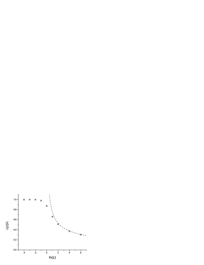
Figure 1: $\lambda(z)/\lambda$ as a function of $ln(z)$ (open circles). Also shown is the asymptotic limit proportional to $1/\sqrt{ln(z)}$ (dashed line).

.

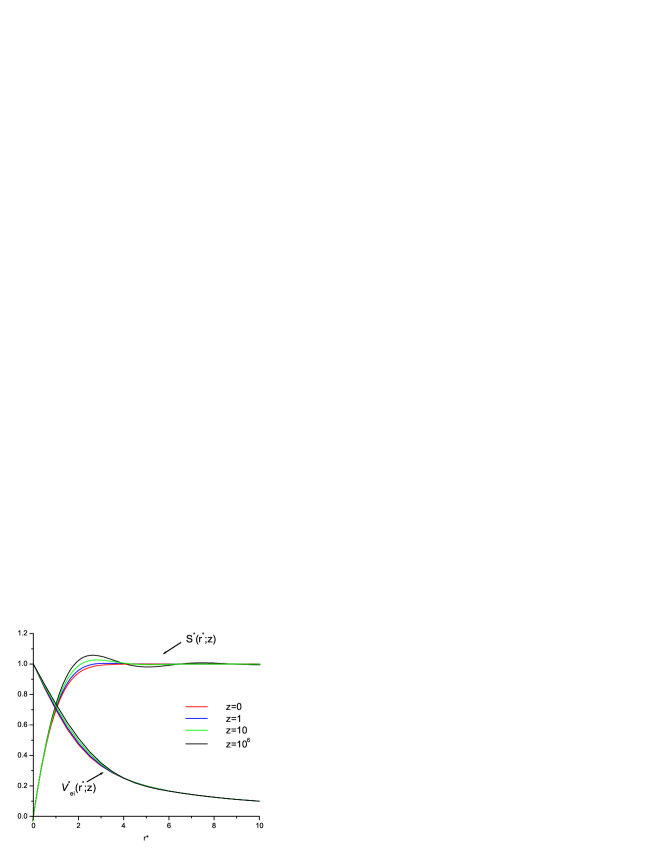
Figure 2: $S^{\ast}(r^{\ast};z)$ and ${\mathcal{V}_{ei}}^{\ast}(r^{\ast};z)$ as functions of $r^{\ast}$ for $z=0,1,10$ and $10^{6}$.

It is interesting to note that the limiting forms (26) and (27) are both scaling functions, scaled by $\lambda$ in the first case and by $\lambda/\sqrt{\ln z}$ in the second case. To explore the extent to which effects of degeneracy can be described by scaling alone, consider the degeneracy dependent wavelength $\lambda\left(z\right)$ defined in (25). For small $z$ it approaches $\lambda$ while for large $z$ it is proportional to $1/\sqrt{\ln z}$ as shown in Figure 1. Hence it is a possible scaling length to interpolate between these limits. Accordingly, define $S^{\ast}(r^{\ast},z)$ by

$$S^{\ast}(r^{\ast}\equiv\frac{r}{\lambda(z)},z)=S(\frac{r}{\lambda},z).$$ (28)

It follows from (25) that this scaling assures that the initial slopes of $S^{\ast}(r^{\ast},z)$ are the same for all $z$ . Figure 2 shows the extent to which this scaling captures the effects of degeneracy for a wide range of $z$. Also shown is the corresponding dimensionless quantum potential $\mathcal{V}_{ei}{}^{\ast}(r^{\ast},z)\equiv{S}^{\ast}(r^{\ast},z)/r^{\ast}$. For large and small $r^{\ast}$ the curves are the same, although there are some differences for intermediate values of $r^{\ast}$. This is due mainly to the oscillatory feature that develops for strong degeneracy (related to Friedel oscillations). However, the quantitative effect on the quantum potential in these scaled units is quite small.

This suggests the approximation for arbitrary degeneracy

$$S^{\ast}(r^{\ast},z)\simeq S^{\ast}(r^{\ast},0),$$ (29)

or correspondingly, the approximate quantum potential

$$\mathcal{V}_{ei}(r)\simeq V(r)S_{K}(\frac{r}{\lambda(z)}).$$ (30)

Here $S_{K}(r/\lambda(z))$ is the non-degenerate Kelbg form of (26), but now with $\lambda$ replaced by $\lambda(z)$. Thus, approximation (30) is a universal function for all degrees of degeneracy. The change in length scale with degeneracy can be understood by noting that the characteristic energy defining this scale is not $k_{B}T$ but rather the average kinetic energy per particle which approaches the Fermi energy for large $z$.

The above explicit results for $\mathcal{V}_{ei}(r)$ are limited to weak coupling. In the case of an attractive ion at the origin there are important bound state effects that are not included in this weak coupling form. However, it has been shown filinov that such strong coupling effects can be included approximately by parameterizing the Kelbg form to fit the exact value of $n(\mathbf{r=0},z=0,\beta)$. The possibility of extending this to $z>0$ in (30) will be explored elsewhere.

IV Summary

One of the simplest quantum systems exhibiting both diffraction and exchange effects is a fixed impurity in an ideal Fermi gas of electrons. Here, a classical system has been associated with that quantum system by the introduction of two quantum potentials. The first is the well-known pair interaction potential among the classical electrons to represent exchange, while the second is a renormalization of the bare impurity-electron interaction. The potentials are defined by the requirement that pair correlations for the classical and quantum systems should be the same. The classical pair potential is determined entirely by the ideal Fermi gas correlation function and describes only exchange effects. The classical electron-impurity potential differs from the bare potential of the quantum system by both exchange and diffraction effects in a complex mixture of the two. A simple representation at weak coupling is given by the familiar Kelbg form for diffraction regularization, but modified by a degeneracy dependent length scale.

Applications of classical molecular dynamics to real systems, such as a hydrogen, require a classical representation with quantum potentials representing both quantum effects and Coulomb interactions among all particles. Current applications use quantum potentials for the electrons that are the sum of an exchange potential $\mathcal{V}_{ee}$ as determined here plus a regularized Coulomb potential of the Kelbg type for diffraction effects. However, the analysis of the impurity problem here suggests that exchange and diffraction are not likely to be additive. This is clear from Eq. (8) where all information about the quantum effects enters via $n_{ee}$ where all effects are mixed (e.g., in the random phase approximation). It is only in the sense of perturbation in one or the other that they become additive.

V Acknowledgements

The research was supported by the NSF/DOE Partnership in Basic Plasma Science and Engineering under the Department of Energy award DE-FG02-07ER54946.

References

- (1) G. Kelbg, Ann. Phys. (Leipzig) 12, 219 (1963); 13, 354 (1963); 14, 394 (1964).
- (2) V.S. Filinov, M. Bonitz, W. Ebeling, and V.E. Fortov, Plasma Phys. Cont. Fusion 43, 743-759 (2001); V. Filinov et al. J. Phys. A: Math. Gen. 36, 6069 (2003).
- (3) R.P. Feynman and H. Kleinert, Phys. Rev. A 34, 5080 (1986); H. Kleinert, Path Integrals in Quantum Mechanics, Statistics and Polymer Physics, 2nd ed. (World Scientific, Singapore, 1995).
- (4) For recent reviews, see A. Filinov, V. Golubnychiy, M. Bonitz, W. Ebeling, and J. Dufty, Phys. Rev. E 70, 046411 (2004); A. Filinov, M. Bonitz, and W. Ebeling, J. Phys. A: Math. Gen. 36, 5957 (2003); W. Ebeling, A. Filinov, M. Bonitz, V. Filinov, and T. Pohl, J. Phys. A: Math. Gen. 39, 4309 (2006).
- (5) D. Bohm, Phys. Rev. 85, 166 and 180 (1986); D.K. Ferry and J. R. Zhou, Phys. Rev. B 48, 7944 (1993).
- (6) A. Fromm, M. Bonitz, and J. Dufty, Annals of Physics 323, 3158 (2008).
- (7) F. Lado, J. Chem. Phys. 47, 5369 (1967).
- (8) J-P Hansen and I. MacDonald, Theory of Simple Liquids, (Academic Press, San Diego, 1990).
- (9) M.W. C. Dharma-wardana and F. Perrot, Phys. Rev. Lett. 84, 959 (2000); F. Perrot and M.W. C. Dharma-wardana, Phys. Rev. B 62, 16536 (2000); M. W. C. Dharma-wardana, Phys. Rev. Lett. 101 035002 (2008).
- (10) C. Jones and M. Murillo, High Energy Density Physics 3, 379 (2007).
- (11) A. L. Fetter and J. D. Walecka, Quantum Theory of Many-Particle Systems (McGraw-Hill, NY, 1963).
- (12) J. Dufty, S. Dutta, M. Bonitz, A. Filinov (unpublished).