ULySS: A Full Spectrum Fitting Package

Abstract

Aims. We provide an easy-to-use full-spectrum fitting package and explore its applications to (i) the determination of the stellar atmospheric parameters and (ii) the study of the history of stellar populations.

Methods. We developed ULySS, a package to fit spectroscopic observations against a linear combination of non-linear model components convolved with a parametric line-of-sight velocity distribution. The minimization can be either local or global, and determines all the parameters in a single fit. We use $\chi^{2}$ maps, convergence maps and Monte-Carlo simulations to study the degeneracies, local minima and to estimate the errors.

Results. We show the importance of determining the shape of the continuum simultaneously to the other parameters by including a multiplicative polynomial in the model (without prior pseudo-continuum determination, or rectification of the spectrum). We also stress the benefice of using an accurate line-spread function, depending on the wavelength, so that the line-shape of the models properly match the observation. For simple models, i. e., to measure the atmospheric parameters or the age/metallicity of a single-age stellar population, there is often a unique minimum, or when local minima exist they can unambiguously be recognized. For more complex models, Monte-Carlo simulations are required to assess the validity of the solution.

Conclusions. The ULySS package is public, simple to use and flexible. The full spectrum fitting makes optimal usage of the signal.

1 Introduction

Spectroscopic data from astronomical sources contain most of the information that we can get from the remote universe, such as physical conditions, composition or motions. Often, the information extraction relies on the identification and analysis of spectral signatures due to more or less well understood physical processes. This is usually an interactive task and requires a specialised expertise, although this is becoming less true with time (e. g., Sousa et al. 2007).

The recent data avalanche prompted a search for automated, objective (and generally more efficient) methods.One possibility is to directly compare an observed spectrum with a set of models or an empirical library of object with known characteristics on a pixel to pixel basis. This can be done for the analysis of stellar atmospheres as in Bailer-Jones et al. (1997), Katz et al. (1998, TGMET), Prugniel & Soubiran (2001), Snider et al. (2001), Willemsen et al. (2005), Shkedy et al. (2007) and Recio-Blanco et al. (2006, MATISSE). It has also been used for the determination of the history of stellar populations as in Heavens et al. (2000, MOPED), Panter et al. (2003), Cid Fernandes et al. (2005, Starlight), Moultaka (2005), Ocvirk et al. (2006b, a, STECKMAP) and Tojeiro et al. (2007, VESPA).

The main advantage of these methods is that, rather than picking specific features, they make optimal usage of the entire measured signal. This comes with a price, however, as we forfeit our ability to draw direct relations between the strength of a specific feature and a physical characteristic. This lack of simplicity should ultimately be regarded as inherent to the nature of the spectra, where the information is redundant and distributed (possibly uniformly) over a large wavelength range.

This paper presents ULySS (Université de Lyon Spectroscopic analysis Software), a new software package enabling full spectral fitting for two astrophysical contexts: The determination of (i) stellar atmospheric parameters and (ii) star formation and metal enrichment history of galaxies. Many similarities between these two cases allowed us to build a single package capable of handling both.

In ULySS, an observed spectrum is fitted against a model expressed as a linear combination of non-linear components, optionally convolved with a line-of-sight velocity distribution (LOSVD) and multiplied with a polynomial function. A component is a non-linear function of some physical parameters (e. g., $T_{\rm eff}$, log($g$) and [Fe/H]). The multiplicative polynomial is meant to absorb errors in the flux calibration, Galactic extinction or any other cause affecting the shape of the spectrum. It replaces the prior rectification or normalization to the pseudo-continuum that other methods requires. This model is compared to the data through a non-linear least-square minimization.

ULySS has been used to study stellar populations (Koleva et al. 2008c; Michielsen et al. 2007; Koleva et al. 2008a; Koleva 2009; Bouchard et al. 2009) and determine atmospheric parameters of stars (Prugniel et al. 2009).

The goal of this paper is to describe the package and to explore the potential and caveat of direct comparison between an observation and a composite model. A previous implementation of the same idea, shortly described earlier and named NBURSTS (Koleva et al. 2007, 2008c), was a variant of the pPXF program (Cappellari & Emsellem 2004, hereafter CE04) applied to stellar populations. Another variant of pPXF was developed by Sarzi et al. (2006) to fit in the same time the stellar and the gas kinematics. The main reason for the name change is the widening of the scope of the package to the measurement of atmospheric parameters and potentially other applications. In addition the algorithm has been modified in some of its mathematical details to improve its precision, robustness and performance. We also made the package user-friendly, wrote documentation and tutorials to allow the public distribution of the package.

The paper is organized as follow: In Sect. 2 we describe the method and the package. In Sect. 3 we illustrate the approach with the case of the determination of the atmospheric parameters of a star. In Sect. 4, we give examples of analysis of a stellar population. The Sect. 5 draws conclusions.

2 Description of the method and package

The method consists in minimizing the $\chi^{2}$ between an observed spectrum and a model. The model is generated at the same resolution and with the same sampling as the observation and the fit is performed in the pixel space. This optimizes the usage of the information, as all the signal is used, and allows easy consideration of the errors on each spectral bin.

The method proceeds in a single fit to determine all the free parameters in order to handle properly the degeneracies between them (e. g., the temperature-metallicity for a stellar spectrum). Other methods estimate the parameters in different steps. For example, one may measure the temperature using criteria almost insensitive to the metallicity and in turn, using this temperature, derive the metallicity. If in fact the criteria to obtain the temperature is somehow metallicity-dependent, the absolute minimum will not be reached unless the fit is iterated. Using a single minimization do not require this additional complexity.

Ocvirk et al. (2006b, a, hereafter STECKMAP) presented another implementation of this approach, using a non-parametric regularized fit. It performs very well to reconstruct the evolution history of a stellar population. But one of its limitation is the difficulty to grant a degree of confidence on the solution (and it is tailored to stellar populations only). This is the main reason which lead us to work on a ‘simpler’ parametric minimization allowing to better understand the degeneracies and the structure of the parameter space by constructing $\chi^{2}$ maps.

The parametric local minimization presented here has been introduced and compared with STECKMAP in Koleva et al. (2008c) in the case of single stellar populations.

2.1 Parametric Model

The observed spectrum, $F_{obs}(\lambda)$, is approximated by a linear combination of $k$ non linear components, CMP, each with weight $W$. This composite model is possibly convolved with a LOSVD and multiplied by an $n^{th}$ order polynomial, $P_{n}(\lambda)$, and summed to another polynomial, $Q_{m}(\lambda)$:

$$F_{obs}(\lambda)=P_{n}(\lambda)\times\bigg{(} {\rm LOSVD}(v_{sys},\sigma,h3,h4)$$

$$\otimes\sum_{i=0}^{i=k}W_{i}\,\,{\rm CMP}_{i}\,(a_{1},a_{2},...,\lambda)\bigg{)}+Q_{m}(\lambda)$$ (1)

The LOSVD is a function of systemic velocity, $v_{sys}$, velocity dispersion $\sigma$ and may include Gauss-Hermit expansion ($h3$ and $h4$, van der Marel & Franx 1993). $\lambda$ is the logarithm of the wavelength (the logarithmic scale is required to express the effect of the LOSVD as a convolution). The CMP_i must be tailored to each problem. For instance, to study a stellar atmosphere, the CMP will be a function of the effective temperature, $T_{\rm eff}$, surface gravity, $g$, and metallicity, [Fe/H]. Or, for a stellar population, it will be a function of age, [Fe/H], and [Mg/Fe], returning the spectrum of a single stellar population (SSP). In general, a CMP is a function of an arbitrary number of physical parameters and of $\lambda$.

The importance of the multiplicative polynomial has been discussed in Koleva et al. (2008c) as it absorbs the effects of an unprecise flux calibration (a common issue in small-aperture spectroscopy) and of the Galactic extinction (which could also be explicitly included in the model as in STECKMAP). The effect of $P_{n}(\lambda)$ is studied in Sect. 3.2 in the particular case of the determination of atmospheric parameters of a star. A similar study was made in Koleva et al. (2008c) in the case of stellar populations. In all the practical cases that we studied, $P_{n}(\lambda)$ was not degenerate with the parameters of the CMP, and high orders could be used (though $n\,\approx\,10$ is often sufficient to obtain an unbiased estimate of these parameters). The optimal value of $n$, which depends mostly on the resolution and wavelength range, can be chosen with ULySS.

The additive polynomial is certainly of a more delicate usage, and is, in most cases, absent from the model. It is indeed degenerate with the intensity, depth or equivalent width of the lines and may bias determinations of the CMP parameters ($T_{\rm eff}$, age or [Fe/H], depending on the context). Such a term may be included to account for data-processing errors (under- or over-subtraction of a smooth background), or may have a physical origin. When determining the stellar kinematics by fitting one or several constant CMPs (i. e., fixed spectra, like stars or models without free parameter) the additive term may be required to absorb the template mismatch (Koleva et al. 2008b). Omitting the additive term would in that case bias the measurement of the velocity dispersion. For this reason, an additive term is generally present in the packages used to determine the internal kinematics of a stellar population. For instance, in CE04 it is an explicit polynomial, or in Fourier quotient programs (Sargent et al. 1977) the spectrum is continuum- or mean-subtracted before the fit and the amplitude or the features is a free parameter (this is equivalent to an additive term). Another place needing an additive term is the analysis of a stellar population in presence of the nebular continuum emission of an AGN (in that case a power-law is more appropriate than a Legendre polynomial; see the tutorial distributed with the package). The biases on the stellar population parameters may be determined from simulations (Prugniel et al. 2005; Prugniel & Koleva 2007).

In summary, we can only advise careful usage of the additive terms. They are only needed in rare circumstances and including them without valid reasons (or failing to do so when they are required) may severely bias the results of the analysis. The lowering of the $\chi^{2}$ that is likely to result from the inclusion of additional degrees of freedom should not be the only criterium to evaluate the validity of the model. The user should check the effects of these terms on the CMP parameters using simulations.

2.2 Algorithm

As written in Eq. 1, the problem is a fit to a multilinear combination of non-linear functions. The parameters of each CMP_i are in general non-linear and are evaluated together as those of the LOSVD with a Levenberg-Marquardt (Marquart 1963; Moré et al. 1980) routine (hereafter LM). To measure the $h3$ and $h4$ coefficients of the LOSVD the package implements the penalization proposed by CE04 to bias them to 0. This option, not illustrated here, is useful to analyse low S/N data.

The (linear) coefficients of the $P_{n}(\lambda)$ and $Q_{m}(\lambda)$ polynomials are determined by ordinary least-square at each evaluation of the function minimized by the LM routine. The weights of each components, $W_{i}$, are also determined at each LM iteration using a bounding value least-square method (Lawson & Hanson 1995) in order to take into account constraints on the contribution of each component, like imposing positivity.

An alternative would have been to use the variable projection method (Golub & Pereyra 1973) for solving this separable nonlinear least-squares problem (i. e. where the model is a linear combination of non-linear functions). We did not use this solution because the bounding of the linear parameters is not possible in the public implementation of this method (Bolstad 1977, the VARPRO program), in addition there was no version of this algorithm in the IDL/GDL language used for this project. Therefore we preferred to adjust the linear parameters in a separate layer at each LM iteration, as in Cappellari & Emsellem (2004). We stress that separating the linear variables is important, not only for performance reasons but also for stability.

The bounding on the $W$ is an option that can be tuned on the particular case of a $CMP$. For example, when dealing with the decomposition of a stellar population as a series of bursts, each component must have a positive or null weight. The LM implementation by Moré et al. (1980, in MINPACK) gives the freedom to also define limits for the values of any of the parameters of the $CMP$.

For $P_{n}(\lambda)$ and $Q_{m}(\lambda)$, we use Legendre polynomial developments of respectively orders $n$ and $m$, for their orthogonality properties. However, the developments intervening in our problem are not strictly orthogonal because (1) the errors are not uniform along the $\lambda$ axis and (2) there may be gaps in the signal corresponding to masked pixels (missing or damaged values). For these reasons, the $P_{n}(\lambda)$ and $Q_{m}(\lambda)$ are determined by an ordinary least square fit. Defining ad’hoc orthogonal polynomials would have been equivalent both from mathematical and performance point of views.

Note that as the LM minimization makes its path to the solution using the local gradients of the CMPs, there is no need or advantage to apply a linear transformation to these functions. For example, applying a rotation in the age – metallicity plan in order to minimize on two orthogonal parameters does not ease the convergence or avoid local minimas: The path to the solution is not affected. But a proper choice of the parameters may lead to a better convergence. For instance, to fit a stellar spectrum, minimizing on log($T_{\rm eff}$) or on $\theta=5040/$$T_{\rm eff}$ is preferrable than using directly $T_{\rm eff}$.

2.3 Line Spread Function

To compare a model to an observation, both must have the same spectral resolution, or we must first transform either the model or the observation in order to match their respective resolution.

The spectral resolution is characterized by the line spread function, LSF, which is the analogous in the spectral direction of the PSF (point spread function) for images. This is the impulse response describing the wavelength distribution of the flux of an un-resolved spectral line. The LSF results from the convolution between the intrinsic resolution of the spectrograph and the slit function. In first approximation, it is represented by $R=l/\Delta(l)$, where $l$ is the wavelength (linear scale) and $\Delta(l)$ is the FWHM of the LSF.

In practice, the LSF may not be defined by a single number. It is not necessarily a Gaussian, and may change with wavelength and position in the field for integral-field or long-slit spectroscopy. Usually, the model has a higher resolution than the observation. Otherwise, the analysis will not make optimal usage of the available information (i. e., the high resolution details in the observed spectrum will not be exploited).

To make the model comparable to the observations, we proceed in two steps. First we have to determine the LSF and then inject it in the model.

2.3.1 Determination of the line-spread function

Figure 1: Effect of using a precise LSF, illustrated with a fit of a Vazdekis/Miles spectrum with a Pegase.HR/Elodie.3.1 SSP component. The top panel shows the spectrum (in black) and the best fit in blue (both are almost superimposed and the black line can be seen only when zooming on the figure), the red line is the multiplicative polynomial. The yellow regions where rejected from the fit (rejection of flagged telluric lines and automatic rejection of outliers). The middle and bottom panel are respectively the residuals from the best fit when (i) assuming a constant Gaussian LSF (in $\lambda$) or (ii) a matched LSF. The continuous green lines mark the 1-$\sigma$ deviation, and the dashed line is the zero-axis. The right side of the graphic expands a small wavelength region, around Ca4227.

The function that we are seeking is the relative LSF between the model (which have a finite resolution) and the observation. It should normally be determined using calibration observations.

Three types of calibrations can be considered:

1. Arc lamp spectra. They are routinely produced during the observations and are used to adjust the dispersion relation and to achieve the wavelength calibration. The slit of the spectrograph is uniformly illuminated with a discharge lamp (like for example He-Ar) producing narrow emission lines. The position of chosen unblended lines are used to fit the dispersion, and the width and shape can be used to determine the LSF.

2. Standard star. Normally any star, except some hot stars with featureless spectra used for the spectrophotometric calibration, can be used to determine the LSF. The observed spectrum may be compared with a high-resolution spectrum of the same star, or with a model of this star, to determine the broadening due the the spectrograph. ULySS can naturally be used to measure this broadening. (Beware that sometimes spectrophotometric standards are observed with a widened slit, and are not usable for LSF calibration).

3. Twilight spectrum. Spectra of the twilight sky are often used to determine the variation of the sensitivity over the field of the spectrograph. These spectra result from the uniform illumination of the slit by a Solar spectrum and can therefore by used as any stellar spectrum to measure the broadening.

The first solution, with arc spectrum, may appear simpler, as it contains bright and well separated emission lines that can be individually fitted with a Gaussian or Gauss-Hermite development. However, there are some caveat with this approach: (i) Few lines are completely unblended and profiles are sensitive to faint unresolved neighboring lines; (ii) The lines are often bright, and use the detector in a regime strongly different than the observations of the astronomical sources, therefore their profile may be affected by some small non-linearities; (iii) The spectrographs are often used close to the undersampling limit (the width of the arc lines are about 2 pixels) and fitting a profiles in these conditions is perilous; (iv) The illumination of the slit is not exactly the same as for the astronomical sources (different optical paths), and (v) this method determines the absolute LSF that needs to be deconvolved from the models’s LSF before using it. We recommend to use this solution only as a sanity control.

The two other solutions use stellar spectra. As the physical models presented in this article are based on empirical libraries of stellar spectra, a proper choice of the calibration stars can make the task of determining the LSF straightforward (the solar spectrum is included in most libraries). If the exact star is not available at the model’s resolution, a similar star, or an interpolated spectrum may be used. Using a stellar spectrum bypasses some of the difficulties met with arc spectra and can gives directly the relative LSF.

There is still an important phenomenon to consider when describing the LSF. Often, the intrinsic resolution of the spectrograph is significantly higher than the actual resolution which is limited by the slit width. As a consequence, the distribution of light within the slit has an effect on the spectrum. In particular, the apparent broadening of a star observed under excellent seeing condition (seeing smaller than the slit) will be smaller that the broadening observed for an extended object (or a star with poor seeing condition). The effective resolution results from the product of the light profile of the object by the slit function, convolved by the intrinsic resolution of the spectrograph.

This effective resolution depends on the observing conditions and on the light profile of the source. It may vary between consecutive exposures. This problem may be difficult to correct and by limiting the knowledge of the instrumental broadening it hampers the measurement of the physical velocity dispersion. In the types of analysis discussed in this paper, this effect preserves the determination of the other parameters (metallicity, age or $T_{\rm eff}$).

Hints for this effect of resolution of an object within the slit may be obtained when comparing the LSF derived with various standard stars and those obtained with twilight spectra.

A practical mean to measure the LSF is to determine the broadening function (cz, $\sigma$ and possibly $h3$ and $h4$) in a succession of small wavelength intervals. For spectra with R = 1000 to 3000, we typically use segments of 200 Å, separated with 100 Å steps (they overlap by half their length).

2.3.2 Injection of the LSF in the model

Because the LSF varies with wavelength, it cannot be injected in the model as a mere convolution. The method we use consists in convolving the models by the series of LSFs determined at some wavelength and then make a linear interpolation in wavelength between the convolved models.

To illustrate the importance of matching the LSF in the spectrum fitting process, we show in Fig. 1 the analysis of a spectrum with a Pegase.HR population model based on the Elodie.3.1 library. The analysed spectrum is a stellar population model from the library of SSPs computed by Vazdekis with the Miles library (Sánchez-Blázquez et al. 2006). The first fit simply assumes a purely Gaussian and constant LSF. The second uses an optimal LSF. The residuals of the first fit are minimal in the center, but become larger at the edges, a zoom in a small region shows that this is due to a misfit (not to noise). Using the proper LSF corrects this defect and the residuals become smoother. In this particular example, despite the considerable effect on the residuals, the incidence on the stellar population parameters is marginal. The precision of the LSF mostly affects the parameters of the LOSVD. By suppressing the LSF mismatch, we can search for other signatures in the residuals which could have been masked otherwise.

The LSF injection also corrects possible inaccuracies in the wavelength calibration. An example of this is shown in Koleva et al. (2008c), where a wavelength calibration systematic distortion affecting the Bruzual & Charlot (2003) models is corrected.

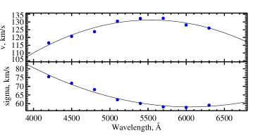
Figure 2: Line spead function of the SDSS.

2.3.3 Example: The SDSS LSF

As an example of LSF analysis, we use the velocity dispersion template stars from the SDSS copied from http://www.sdss.org/dr5/algorithms/veldisp.html. These 32 G and K giant stars from M67 were used to determine the velocity dispersion of the galaxies as an average between estimates obtained by Fourier-fitting and direct-fitting methods.

In Fig. 2 we show the LSF relative to the Elodie.3.1 library obtained with ULySS (Elodie.3.1 is restricted to the wavelength range 3900–6800 Å). It was determined using wavelength intervals of 600 Å spaced by 300 Å. The variation of the instrumental velocity dispersion ($\sigma_{ins}$) with wavelength is significant: from 50 to 75 km s^-1.

The classical methods for measuring the (physical) velocity dispersion, $\sigma$, (Sargent et al. 1977; Tonry & Davis 1979; Franx et al. 1989; Bender 1990; Rix & White 1992; van der Marel & Franx 1993; Cappellari & Emsellem 2004) compares the observation to stellar templates observed with the same setup. As in general, the LSF changes are moderate, the red-shift of the galaxy does not affect significantly $\sigma$ for nearby galaxies. But for a distant galaxy, neglecting the shift of the LSF may give a measurable effect. For a low-mass galaxy with $\sigma$ = 50 km s^-1 measured with the SDSS, the bias would be about 0.1 km s^-1 at z=0.03 but 2 km s^-1 at z=0.4.

2.4 Description of the ULySS package

ULySS, available at http://ulyss.univ-lyon1.fr/, has been programmed in IDL/GDL language. This is the language of the widely used proprietary IDL (Interactive Data Language) software. The open source GDL (Gnu Data Language) interpretor can also be used to run ULySS. The choice of this programming language is essentially historical: Many of the required routines were already available as public libraries and development was started from the pPXF package (Cappellari & Emsellem 2004). We may offer a version written in a modern language (most likely Python) in the future.

ULySS contains various programs and subroutines that can be used for:

• Defining the array of components to fit

• Performing the fit

• Visualising the results

• Making $\chi^{2}$ maps, convergence maps and Monte-Carlo simulations

• Reading data from FITS files

• Testing the package

The package contains extensive documentation and tutorials. The emphasis was put on the flexibility and ease of use.

The package contains routines to define various types of CMPs, notably to analyse a stellar atmosphere (TGM) and to analyse a stellar population (SSP), and the construction of other CMPs by the user was made as easy as possible. To fit a composite model, i. e., a linear combination of components, one simply has to concatenate several CMPs in a single array.

The core of the package is the local minimization described in Sect. 2. Such a minimization starts from a point (guess) in the parameters space, whose choice may be critical. To release this constraint, ULySS makes it easy to perform a global minimization by providing vectors instead of scalars as guesses.

The most valuable aspect of the package is the possibility to explore and visualize the parameters space. The tools offered for that purpose are (i) Monte-Carlo simulations (ii) convergence maps, and (iii) $\chi^{2}$ maps.

Monte-Carlo simulations are performed to estimate the biases, the errors and the coupling (degeneracies) between the parameters. A simple option in the main fitting program allows to perform a series of minimizations with random noise added to the data. This noise has the same characteristics as the one estimated in the data. Normally the noise should be carried throughout the data-reduction process, starting from the statistical noise of the detector that can usually be securely estimated. During the data reduction, the signal is likely to be resampled, when the spectra are extracted from the initial 2D frame, and when they are calibrated in wavelength (or logarithm of wavelength). This operation introduces a correlation between the pixels (see de Bruyne et al. 2003), which is represented in ULySS by the ratio between the actual number of pixels and the number of independent pixels. Using it, the Monte-Carlo simulations reproduces the correct noise spectrum and gives a robust estimates of the errors.

Convergence maps are tools to evaluate the convergence region, i. e., the domain of the parameter space from which guesses converge to the absolute minimum of the $\chi^{2}$. These maps can be generated using the global minimization approach explained above.

$\chi^{2}$ maps are visualizations of the parameters space. They are generated by (i) choosing a 2D projection (e. g., age and metallicity) and a node grid in this plan and (ii) performing an optimization over all the other axes of the parameters space for each node of this grid. These maps allow the identification of degeneracies and local minima.

Typically, when approaching a new problem, like using a new CMP, or a new wavelength range or region of the parameters space, these three tools can be used to understand the reliability of the results before proceeding to the analysis of a massive dataset. Their usefulness are presented in the next sections.

3 Determination of stellar atmospheric parameters

The effective temperature, $T_{\rm eff}$, surface gravity, log($g$), and metallicity, [Fe/H], are fundamental characteristics that can be derived from spectroscopic analysis (Cayrel de Strobel et al. 2001). Full spectrum fitting, as provided by ULySS, can be used for this purpose: The program will identify the best matching $T_{\rm eff}$, log($g$) and [Fe/H] by comparing to a model.

ULySS does a parametric minimization. So, the core of the problem is to obtain a parametric model, i.e. a function returning a spectrum given a set of atmospheric parameters. The reference spectra are either a grid of theoretical models (e. g. Munari et al. 2005; Coelho et al. 2005) or a set of observed stars whose parameters are known from the analysis of individual high resolution spectra (e. g. Soubiran et al. 1998). ULySS requires an interpolator of this grid. In the present paper, we use the one presented in Prugniel & Soubiran (2001) for the ELODIE library. Shortly, it consists in polynomial approximations of the library. Three overlapping ranges of $T_{\rm eff}$ are considered (hot, warm and cold) and linearly interpolated to produce the final function. In each $T_{\rm eff}$ range each pixel of the spectrum is computed as a 21 terms polynomial in $T_{\rm eff}$, log($g$) and [Fe/H]. The coefficients of these polynomials were fitted over the 2000 spectra of the library. The choice of the terms, of the $T_{\rm eff}$ limits and of weights were fine-tuned to minimize the residuals between the observations and the interpolated spectra. In this paper, we use the interpolator built on the continuum normalized spectra. An alternative solution to this global polynomial representation of the library, would have been to use a local approximation based on a gaussian-kernel smoothing, as in Vazdekis et al. (2003, Appendix B).

ULySS defines a model component (CMP in Eq. 1) for this model. The TGM component, as we named it, allows to perform the minimization on the three atmospheric parameters. With the current version of the ELODIE library (Prugniel et al. 2007b, version 3.1) the temperature range is limited to 3 600 K$<$ $T_{\rm eff}$ $<$30 000 K. In the future versions (Wu 2009, in preparation), a greater number of hot ($T_{\rm eff}$ $>$ 10 000 K) and cold ($T_{\rm eff}$ $<$4 200 K) stars will be included, extending the current validity range of the interpolator.

3.1 TGM Fit Example

We analysed the 18 stars from the CFLIB (indo-US, Valdes et al. 2004) library of spectra in common with the study by da Silva et al. (2006) of G & K stars using R$\approx$50000 spectroscopy and LTE models. We performed a fit with a TGM component starting from a grid of guesses in order to be independent of the prior knowledge of the parameters. The LSF was determined by using several stars in common between CFLIB and the ELODIE library. The results found with ULySS are consistent with those of da Silva et al. (2006), Fig. 3, except for HD 189319 where we find a significant discrepancy in metallicity. The measurements from da Silva et al. (2006) are: $T_{\rm eff}$=3978 K log($g$)=1.10 g.cm^-2, [Fe/H]=-0.29 and from ULySS: $T_{\rm eff}$=3904, log($g$)=1.77, [Fe/H]=0.10. It is the most discrepant star for both metallicity and gravity; it is also the lowest gravity and coolest star of this sample. Another recent spectroscopic analysis gives: $T_{\rm eff}$=4150 log($g$)=1.70 [Fe/H]=-0.41 (Hekker & Meléndez 2007); and interferometric measurements tend to indicate a lower $T_{\rm eff}$: 3650 – 3800 K, and hence probably lower gravity log($g$)= 0.9 (Neilson & Lester 2008; Wittkowski et al. 2006). This discrepancy is therefore not raising suspicion concerning ULySS, but the ELODIE interpolator surely merits to be improved in this region of the HR diagram.

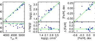
Figure 3: Comparison of the atmospheric parameters determined by ULySS with those from high resolution spectra (da Silva et al. 2006). The abscissas are the measurements from da Silva et al. (2006). On the top panels, the ordinates are from ULySS and the green lines are the diagonals. On the bottom panels the ordinates are the differences ULySS- literature.

For this sample we found $\Delta(T_{eff})/T_{eff}=-0.013\pm 0.010$ (i. e., $60\pm 45$K), $\Delta(log(g))=0.14\pm 0.22$ and $\Delta([Fe/H])=0.01\pm 0.11$. Excluding the discrepant M star we obtain: $\Delta([Fe/H])=-0.01\pm 0.07$. The deviations reported here are the standard deviations on individual measurements. The temperatures found by ULySS are systematically cooler by 60 K than those of da Silva, consistently with the offset mentioned by these authors in their own comparison to the literature. They found a systematic difference of 39 to 50 K, their measurements being hotter. The three atmospheric parameters error estimates from our program are similar to those given by MC simulations and are about 20 times smaller than the ‘external’ errors, so we did not put error bars in Fig. 3, nevertheless the deviations (external errors) are identical to those reported by da Silva et al. (2006). We can conclude that the measurements performed with ULySS are precise and reliable.

Table 1: Stellar atmospheric parameter values for six stars from CFLIB representative of various MK classes. The atmospheric parameters on the first line are compiled from the literature, and on the second line fitted by ULySS.

Name	Sp.Type	$T_{\rm eff}$	log($g$)	[Fe/H]	Ref.
		(K)	g.cm-2.s-1	(dex)
HD30614	O9.5Iae	29647	3.05	0.30	1
		33972	3.18	-0.05
HD195324	A1Ib	9300	1.90	-0.11	2
		9847	1.94	-0.16
HD114642	F5.5V	6434	3.83	-0.12	3
		6431	4.04	-0.12
HD76151	G2V	5768	4.45	0.06	4
		5728	4.41	0.09
HD10780	K0V	5359	4.44	0.02	4
		5330	4.50	0.06
HD42475	M1Iab	4000	0.70	-0.36	5
		3988	0.32	0.02

Litterature source for the atmospheric parameters.

• References — (1) Takada (1977); (2) Venn (1995); (3) Takeda (2007); (4) Soubiran et al. (2008); (5) Luck & Bond (1980).

In Table 1 we selected six CFLIB stars representative of the various spectral types and luminosity classes. Fig. 4 presents the fit for a Solar type star from this list. A detailed discussion of the CFLIB stellar library will be made in a separate work.

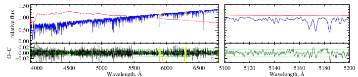
Figure 4: Fit of the CFLIB star HD 76151 with a TGM component. The symbols and conventions are same as in Fig. 1. The order of the multiplicative polynomial is $n=$200. The right side expands a small wavelength region around Mg_b.

3.2 Multiplicative polynomial continuum

Most stellar analysis programs first require the observed spectrum to be normalized to a pseudo-continuum, which can be determined either interactively or automatically. By contrast, ULySS determines this normalization in the same fitting process by including a multiplicative polynomial, $P_{n}(\lambda)$ in Eq. 1, in the model. This single-step fitting procedure insures that the minimum $\chi^{2}$ can be reached and allows to check the possible dependences between this continuum and the measured physical parameters.

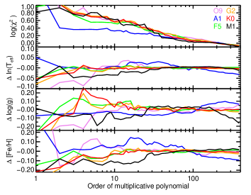
Figure 5: The evolution of the stellar atmospheric parameters fit results ($\chi^{2}$, log($T_{\rm eff}$), log($g$), and [Fe/H]) with increasing Legendre polynomial degree for 6 example CFLIB stellar spectra. Black, green, red, blue, violet and gold colors are respectively standing for each star listed in table 1.

Figure 5 presents the results of a series of fits of the six representative stars from Table 1 varying the order of $P_{n}(\lambda)$. The observations consist in 8300 independent pixels in the wavelength range 3900 – 6800 Å. As there is no external estimate of the noise, we affected a constant weight to all the pixels (except those rejected as outliers), and computed the noise in order to reach $\chi^{2}$=1 for $n$=200. We explored the multiplicative polynomial order range $0<n<800$, while $n$ increasing, the value of the $\chi^{2}$ decreases as a power law.

The atmospheric parameters converge rapidly to their asymptotic values (defined here as the mean of the solutions for $n>25$). For the F, G, K and O stars the plateau is reached between $n=$10 to 15 (the stability of the solution is lower for the O star, in particular for metallicity). For the M star, the plateau is reached at $n$ = 35, but the fit is not stable above $n$=150. The A1Ib spectral type CFLIB star HD 195324 displays a significant dependence between $n$ and the measured metallicity; it did not stabilize to a plateau. This is likely due to the limited quality of the ELODIE V3.1 interpolator in this under-populated region of the parameters space. The ELODIE library counts only five A-type supergiants and therefore the interpolation is not secure. Besides, in A-type stars the ELODIE continuum are taken in the flanks of the Balmer lines and the analysis rely on the multiplicative polynomial to fit them. We expect that using a flux-calibrated model and an improved library would improve the situation.

Note, that the variations of the parameters with $n$ are slightly larger than the error bars. On respectively $T_{\rm eff}$, log($g$) and [Fe/H] the errors are typically 0.1%, 0.006 and 0.005 while the dispersion of the values for $n>20$ are 0.2%, 0.01 and 0.01, i. e. about twice the errors. The extremely small internal errors hide some potential biases of either observational or physical origin.

Another evidence for the non-degeneracy between the atmospheric parameters and $n$, even for values of $n$ considerably larger than what is used in practical cases, is given by the Monte-Carlo simulations of the next section. In the case of degeneracy, the error bars computed by the fitting program would be underestimated.

In order to check if the high values of $n$ are over-fitting the data (i. e. fit the noise), we made similar experiments with noise spectra having the same characteristics as the data. The measured $\chi^{2}$ decreases as expected, to reach 0.99 for $n=100$, 0.98 for $n=400$ and 0.96 for $n=800$. It is clear that the $\chi^{2}$ trend seen for the observation is not due to the over-fitting, as the slope is much larger. The decrease of $\chi^{2}$ is probably due to the shape of the continuum increasingly better fitted when $n$ rises, and to some extent the physical effects ignored by this simple model. The effect of rotation for hot stars may be the main influence, moreover detailed abundances are certainly can not be mimiced by the multiplicative polynomial.

The importance of this multiplicative polynomial for stellar population studies is discussed in Koleva et al. (2008c). Within the same wavelength range, the fits reach a plateau for lower $n$, probably because of the models are flux calibrated.

3.3 Convergence, $\chi^{2}$ maps and Monte-Carlo simulations

ULySS also includes the tools to assess the significance and validity of the results. Fig. 6 & 7 illustrate the usage of convergence maps, Monte-Carlo simulations and $\chi^{2}$ maps to explore the space of parameters.

The convergence map, Fig. 6, shows two convergence basins. In the wide region defined by $T_{\rm eff}$ $<$ 10000 K, any choice of initial guess will converge toward the correct solution, while hotter guess temperature may fall into a local minimum in an unphysical region.

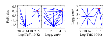
Figure 6: Convergence maps on different projections of the parameters space for the CFLIB star HD 76151 inverted with the TGM component. Red crosses stand for the global minimum solutions found by ULySS.

Monte-Carlo simulations are used to estimates the errors when the different parameters are not independent. The errors determined by Monte-Carlo simulations are compared in Fig. 7 with those given by the minimization procedure. Though both are in approximate agreement, only the simulations can render the effect of the coupling of the errors between the parameters. The simulations consist in series of analyses of a spectrum plus a random noise corresponding to the estimated noise. The added noise has a Gaussian distribution and take into account the correlation between the pixels introduced along the processing as stressed by de Bruyne et al. (2003). This latter effect is modeled by keeping track of the number of independent pixels along the steps of the processing, and then generating a random vector of independent points that is finally resampled to the actual length of the spectrum.

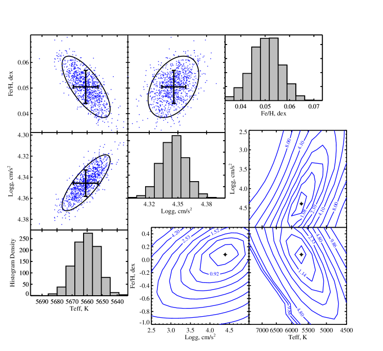
Figure 7: Monte-Carlo simulations and $\chi^{2}$ maps for the CFLIB star HD 76151 inverted with the ELODIE library as presented in Fig. 4. The three projections of the parameters space are presented. The 1000 Monte-Carlo simulations are performed adding a random noise equivalent to the estimated one. The overimposed crosses figure the internal errors estimated by ULySS, and the ellipses the standard deviation computed from the simulations.

The $\chi^{2}$ maps complete the Monte-Carlo simulations by unveiling the degeneracies and the presence of local minimas. We built them by choosing a grid of nodes in a 2 dimensional projection of the parameters space, and performing the minimization for each node (hence optimizing n-2 parameters). Any local minimum can be detected, providing that the grid is fine enough. The topology of these maps also indicates the degeneracies. In the case presented by Fig. 7, measurement of the three atmospheric parameters for a Solar type star, the maps are regular, showing weak dependences between the parameters and a single minimum. When using more complex models, like composite stellar population, the maps often show local minimas.

4 History of stellar populations

By using the SSP component (single stellar population) provided with ULySS, one can evaluate many evolutionary parameters from an integrated spectra. As in the case of the TGM component, the SSP component describes the fitting boundaries and the overall recipe to create SSP spectra and fit them onto the observed data. This time, the CMP is characterised by age, [Fe/H] and [Mg/Fe] (this last dimension is currently only available in semi-empirical models under development, see Prugniel et al. 2007a). A grid of SSPs given in input is spline-interpolated to provide a continuous function.

The CMPs can be linked to a number of population synthesis models. Koleva et al. (2008c) tested 3 of them: Galaxev (Bruzual & Charlot 2003), Pegase.HR (Le Borgne et al. 2004) and Vazdekis-Miles (Vazdekis 1999; Sánchez-Blázquez et al. 2006). They concluded that Pegase.HR and Vazdekis-Miles are reliable and consistent.

The first step towards reconstructing the star formation history (SFH) of an object is to calculate its SSP-equivalent parameters by using a single CMP that interpolate a grid of SSP in age, [Fe/H] and possibly [Mg/Fe]. These SSP-equivalent parameters correspond (more or less) to the luminosity weighted average over all the population that can have a distribution in age and metallicity. The present analysis program has been used by Koleva et al. (2008c) who has shown that reliable information can be retrieved. The metallicity of Galactic globular clusters can be compared to the determinations derived from spectroscopy of individual stars with a precision of 0.1 dex, which is the actual precision of these latter measurements.

If the object has a complex SFH, with several epochs of star formation, SSP-equivalent parameters are essentially representative of the star formation burst that dominates the light (often the more recent). The ULySS package can be used to reconstruct a detailed SFH, in practice limited to 2 to 4 epochs of star formation (see also VESPA; Tojeiro et al. 2007).

4.1 Complex Stellar Population: Application to NGC205

The galaxies have in general a complex SFH and retracing the star formation rate along the history is a fundamental information for the physics of the galaxies and for the cosmology. In principle, one can access such information by fitting directly a positive linear combination of many SSPs, but such approach would be unstable because of the degeneracies between the components and require a regularization.

To circumvent these degeneracies, we start with simple physical assumptions, like the presence of an old stellar population, then divide the time axis in intervals (by setting limits in two or more intervals). As the number of free parameters raise, local minima appear and global minimization are required; the $\chi^{2}$ maps help to understand the structure of the parameters space. Usually the fit is performed several times, with increasing number of components and varying limits on the population boxes. Then, doing Monte-Carlo simulations and checking the residuals of the fits, it is possible to assess the relevance of the solutions and select the most probable SFH.

As an example, we analyse the star formation in the inner 2″ (roughly the size of the nucleus, Butler & Martínez-Delgado 2005) of NGC 205. The data, taken from Simien & Prugniel (2002), have S/N $\approx$ 50 in the central region and spectral resolution of R $\sim$ 5000. For this present demonstration, we analyse this spectrum in terms of two epochs of star formation (i. e., 2 CMPs, each one being an SSP): one ‘young’ (age $<$800 Myr) and one ‘old’ (800 $<$ age $<$ 14 000 Myr). This hypothesis is not bound to an a priori knowledge of the stellar population; it is essentially a choice of time resolution. Depending on S/N, resolution and wavelength range, the number of components may be increased; e. g., in Koleva (2009) the same data are decomposed in four epochs of star formation.

Table 2: Ages and metallicities of the central $2^{\prime\prime}$ of NGC205. The first part of the table give the direct fits, for one and two SSPs. The second part give the mean values and standard deviations derived from 1000 Monte Carlo simulations. In this second part, MC1 is the result of the Monte-Carlo analysis of the SSP direct solution with a 2-SSP models.

SSP	$\chi^{2}$	$age$	[Fe/H]	$f_{mass}$	$f_{light}$
		(Gyr)	(dex)
1 / 1	1.37	1.27$\pm$0.02	-0.67$\pm$0.02	-	-
1 / 1	MC	1.27$\pm$0.02	-0.67$\pm$0.02	-	-
1 / 2	1.22	0.13$\pm$0.02	0.29$\pm$0.07	0.06$\pm$0.00	0.25$\pm$0.00
2 / 2		1.81$\pm$0.08	-0.73$\pm$0.01	0.94$\pm$0.00	0.75$\pm$0.00
1 / 2	MC	0.14$\pm$0.04	0.28$\pm$0.04	0.07$\pm$0.02	0.26$\pm$0.04
2 / 2		1.90$\pm$0.36	-0.74$\pm$0.08	0.93$\pm$0.07	0.74$\pm$0.04
1 / 2	MC1	-	-	-	-
2 / 2		1.30$\pm$0.03	-0.67$\pm$0.04	-	-

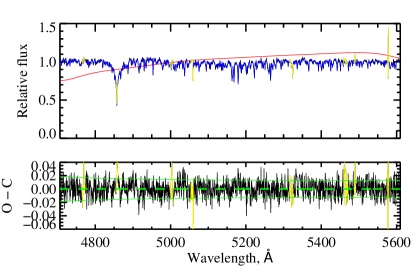
Figure 8: Fit result for the central 2^′′ of NGC 205 with 2 SSP components. In the top panel the black line represents the observed spectra, the blue line is the fitted model and the red line shows the multiplicative polynomial ($P_{n}(\lambda)$). The bottom panel shows the residuals (black), mean (green dashed) and 1$\sigma$ deviation (solid green). In both panels, some of the data were not considered for the fit (yellow).

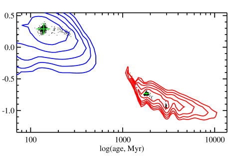
Figure 9: Monte-Carlo simulation (dots) and $\chi^{2}$ map (contours) for a 2 CMP fit to spectra of the inner 2″ of NGC 205. The blue contours represents the $\chi^{2}$ levels for the young stellar population (age constrained to be $<800$ Myr) and the red contours are for the old population (age between 800 and 14 000 Myr).

Figure 8 and Table 2 shows the results of our analysis. For the young component we find an age of $\sim$130 Myr consistent with photometric results (J, H, K photometry) from Davidge (2003) and with Cepa & Beckman (1988) who found from orbital considerations that NGC 205 crossed the disk of M31 about 100 Myr ago. It represents about 25% of the light and only about 7% of the mass.

The Monte-Carlo simulations of Fig. 9 show that we can distinguish between the two populations, in the sense that the two clouds corresponding to these populations are well separated. However, the existence of two bursts was one of our hypotheses and to test its validity we will apply the same analysis to the best fit SSP of the first NGC 205 experiment. We find that a young burst would be detected in about 10% of the cases in Monte-Carlo simulations, but it is easily rejected as the solution does not cluster around a marked minimum.

The mean solutions estimated from the Monte-Carlo simulations with two bursts, given in Table 2 (lines noted ’MC’ in the $\chi^{2}$ column), are compatible with the direct fit, but the errors are significantly larger (because of the degeneracies). It is also interesting to see that the analysis with a 2-bursts model of the best-fit SSP produce an unbiased solution (lines noted ’MC1’).

Examining Fig. 9 in more details, we note that the distribution of the Monte-Carlo solutions are not simple Gaussians centered on the direct solution. For the old burst, there is a small and concentrated secondary cloud gathering 10% of the solutions at an age of about 3 Gyr and [Fe/H]=-1. The solutions belonging to that cloud form also a tail at the old side of the young burst. This feature is associated to a local minimum detected on the $\chi^{2}$ map whose depth is almost similar to the solution. Because of the random noise, this local minimum can become the actual solution. It means that the two minima cannot be statistically distinguished. The morphology of the map gives the impression that the oldest cloud is an artifact due to a discontinuity of the model (either in the population model of interpolation of the Elodie spectra). But there is no objective argument to reject this (less probable) solution.

4.2 Exponentially declining or constant SFR populations

Our last series of experiments consists in analysing simulated populations with an extended star formation history. We consider here two scenarios: a constant star formation rate (SFR) stopped 500 Myr ago and an exponentially declining SFR with a characteristic time, $\tau$, of 5 Gyr. These spectra were computed with Pegase.HR and ELODIE.3.1. In both cases we analysed the simulated galaxies with a model made of 3 CMPs defined by the age limits: [12,800], [800, 5000], [12000] Myr. The goal is to see if we can distinguish between different scenarios of star formation.

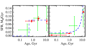
Figure 10: Star formation histories of two simulated populations with constant (upper panel) and exponentially decreasing (lower panel) star formation rates. The vertical axis is the SFR normalized to a total mass of formed stars equal to 1 M_⊙. The blue dashed lines represents the simulated star formation. The red squares are the direct solution of the fit to a 3 SSPs model. The green crosses are the results from MC simulations (200 inversions with S/N=50).

We fitted the direct solutions (without noise) and we made a series of 200 inversions with different realization of the added noise corresponding to S/N=50. Fig.10 presents the results as the SFR versus time. For both simulated populations we find significant contribution (more than 10% in light) in the youngest component box, where the star formation had the lowest rate. The SFR reconstructions reproduce well the simulated histories and the MC simulations agree with the direct solution within the uncertainties. The direct solution underestimates the error bars due to the degeneracies between the ages and the relative weights of each component.

The error bars on the age are larger than in the case of NGC 205. In fact the individual solutions of the MC realizations span the whole age range allowed for each of the components. This may be an indication that by contrast, the star formation history of NGC 205 is marked by a recent short burst rather than a smoothly declining SFR.

5 Conclusion

We presented the ULySS packages and its applications to the analysis of stellar atmosphere and stellar population spectra. This packages is simple to use and is an efficient tool to determine the atmospheric parameters of stars ($T_{\rm eff}$, log($g$) and [Fe/H]). The convergence region and the degeneracies can be studied in details and the errors on estimated parameters are robustly determined. ULySS is also used to recover the history of star formation in galaxies and stellar clusters by decomposing the observed spectrum as a series of SSPs. The simultaneous analysis of the kinematics and of the stellar mix of a population allows to break degeneracies and gain in reliability and precision on both the kinematics and the star formation history.

ULySS is available for download (http://ulyss.univ-lyon1.fr). Beside the applications described in the present paper, it contains other components (e. g. LINE, used to fit emission lines) and can easily be extended to other applications.