A Vector Generalization of Costa’s Entropy-Power
Inequality with Applications

Abstract

This paper considers an entropy-power inequality (EPI) of Costa and presents a natural vector generalization with a real positive semidefinite matrix parameter. This new inequality is proved using a perturbation approach via a fundamental relationship between the derivative of mutual information and the minimum mean-square error (MMSE) estimate in linear vector Gaussian channels. As an application, a new extremal entropy inequality is derived from the generalized Costa EPI and then used to establish the secrecy capacity regions of the degraded vector Gaussian broadcast channel with layered confidential messages.

I Introduction

In information theory, the entropy-power inequality (EPI) of Shannon [1] and Stam [2] has played key roles in the solution of several canonical network communication problems. Celebrated examples include Bergmans’s solution [3] to the Gaussian broadcast channel problem, Leung-Yan-Cheong and Hellman’s solution [4] to the Gaussian wire-tap channel problem, Ozarow’s solution [5] to the Gaussian two-description problem, Oohama’s solution [6] to the quadratic Gaussian CEO problem, and more recently Weingarten, Steinberg and Shamai’s solution [7] to the multiple-input multiple-output Gaussian broadcast channel problem.

Let $\mathbf{X}$ and $\mathbf{Z}$ be two independent random $n$-vectors with densities in ${\mathbb{R}}^{n}$, where ${\mathbb{R}}$ denotes the set of real numbers. The classical EPI of Shannon [1] and Stam [2] can be written as

$$\exp\left[\frac{2}{n}h(\mathbf{X}+\mathbf{Z})\right]\geq\exp\left[\frac{2}{n}h(\mathbf{X})\right]+\exp\left[\frac{2}{n}h(\mathbf{Z})\right]$$ (1)

where $h(\mathbf{X})$ denotes the differential entropy of $\mathbf{X}$. The equality holds if and only if $\mathbf{X}$ and $\mathbf{Z}$ are Gaussian and with proportional covariance matrices.

In network information theory, most applications focus on the special case of (1) where one of the random vectors is fixed to be Gaussian. In this setting, the classical EPI of Shannon and Stam can be further strengthened as shown by Costa [8]. Let $\mathbf{Z}$ be a Gaussian random $n$-vector with a positive definite covariance matrix, and let $a$ be a real scalar such that $a\in[0,1]$. Costa’s EPI [8] can be written as

$$\exp\left[\frac{2}{n}h(\mathbf{X}+\sqrt{a}\mathbf{Z})\right] \geq(1-a)\exp\left[\frac{2}{n}h(\mathbf{X})\right]+a\exp\left[\frac{2}{n}h(\mathbf{X}+\mathbf{Z})\right]$$ (2)

for any random $n$-vector $\mathbf{X}$ independent of $\mathbf{Z}$. The equality holds if and only if $\mathbf{X}$ is also Gaussian and with a covariance matrix proportional to that of $\mathbf{Z}$’s.

Though not as widely known as the classical EPI of Shannon and Stam, Costa’s EPI has found useful applications in deriving capacity bounds for the Gaussian interference channel [9] and the multiantenna flat-fading channel [10]. The original proof of Costa’s EPI provided in [8] was based on rather detailed calculations. Simplified proofs based on a Fisher information inequality [11] and a fundamental relationship between the derivative of mutual information and minimum mean-square error (MMSE) in linear Gaussian channels [12] can be found in [13] and [14], respectively.

Note that Costa’s EPI (2) provides a strong relationship among the differential entropies of three random vectors: $\mathbf{X}$, $\mathbf{X}+\sqrt{a}\mathbf{Z}$ and $\mathbf{X}+\mathbf{Z}$. To apply, the increments of $\mathbf{X}+\sqrt{a}\mathbf{Z}$ and $\mathbf{X}+\mathbf{Z}$ over $\mathbf{X}$ need to be Gaussian and have proportional covariance matrices. For some applications in network information theory (as we will see shortly), the proportionality requirement may turn out to be overly restrictive. A main contribution of this paper is to prove a natural generalization of Costa’s EPI (2) by replacing the real scalar $a$ with a positive semidefinite matrix parameter. The result is summarized in the following theorem.

Theorem 1 (Generalized Costa’s EPI)

Let $\mathbf{Z}$ be a Gaussian random $n$-vector with a positive definite covariance matrix $\mathbf{N}$, and let $\mathbf{A}$ be an $n\times n$ real symmetric matrix such that $0\preceq\mathbf{A}\preceq\mathbf{I}$. Here, $\mathbf{I}$ denotes the $n\times n$ identity matrix, and “$\preceq$” denotes “less or equal to” in the positive semidefinite partial ordering between real symmetric matrices. Then,

$$\exp\left[\frac{2}{n}h(\mathbf{X}+\mathbf{A}^{\frac{1}{2}}\mathbf{Z})\right] \geq|\mathbf{I}-\mathbf{A}|^{\frac{1}{n}}\exp\left[\frac{2}{n}h(\mathbf{X})\right]+|\mathbf{A}|^{\frac{1}{n}}\exp\left[\frac{2}{n}h(\mathbf{X}+\mathbf{Z})\right]$$ (3)

for any random $n$-vector $\mathbf{X}$ independent of $\mathbf{Z}$. The equality holds if $\mathbf{Z}$ is Gaussian and with a covariance matrix $\mathbf{B}$ such that $\mathbf{B}-\mathbf{A}\mathbf{B}$ and $\mathbf{B}+\mathbf{A}^{\frac{1}{2}}\mathbf{N}\mathbf{A}^{\frac{1}{2}}$ are proportional.

Note that when $\mathbf{A}=a\mathbf{I}$, the generalized Costa EPI (3) reduces to the original Costa EPI (2). On the other hand, when $\mathbf{A}$ is not a scaled identity, the covariance matrices of increments of $\mathbf{X}+\mathbf{A}^{\frac{1}{2}}\mathbf{Z}$ and $\mathbf{X}+\mathbf{Z}$ over $\mathbf{X}$ do not need to be proportional. As we will see, the ability to cope with a general matrix parameter makes the generalized Costa EPI more flexible and powerful than the original Costa EPI.

A different but related generalization of Costa’s EPI was considered by Payaró and Palomar [15], where they examined the concavity of the entropy-power $\exp\left[\frac{2}{n}h(\mathbf{A}^{\frac{1}{2}}\mathbf{X}+\mathbf{Z})\right]$ with respect to the matrix parameter $\mathbf{A}$. This line of research was motivated by the observation that the original Costa EPI (2) is equivalent to the concavity of the entropy power $\exp\left[\frac{2}{n}h(\sqrt{a}\mathbf{X}+\mathbf{Z})\right]$ with respect to the scalar parameter $a$. Unlike the scalar case, Payaró and Palomar [15] showed that the entropy-power $\exp\left[\frac{2}{n}h(\mathbf{A}^{\frac{1}{2}}\mathbf{X}+\mathbf{Z})\right]$ is in general not concave with respect to the matrix parameter $\mathbf{A}$. However, the concavity does hold when $\mathbf{A}$ is restricted to be diagonal [15].

In information theory, a main application of the EPI is to derive extremal entropy inequalities, which can then be used to solve network communication problems. In their work [16], Liu and Viswanath derived an extremal entropy inequality based on the classical EPI of Shannon [1] and Stam [2] and used it to establish the private message capacity region of the vector Gaussian broadcast channel via the Marton outer bound [17, Theorem 5]. In this paper, we will derive a new extremal entropy inequality based on the generalized Costa EPI and use it to characterize the secrecy capacity regions of the degraded vector Gaussian broadcast channel with layered confidential messages.

The rest of the paper is organized as follows. In Section II, we summarize the main results of the paper, including a new extremal entropy inequality and its applications on the degraded vector Gaussian broadcast channel with layered confidential messages. In Section III, we prove the generalized Costa EPI, following a perturbation approach via a fundamental relationship between the derivative of mutual information and MMSE estimate in linear vector Gaussian channels [18, Theorem 2]. In Section IV, we derive the new extremal entropy inequality from the generalized Costa EPI. The coding theorems for the degraded vector Gaussian broadcast channel with layered confidential messages are proved in Section V and Section VI. Finally, in Section VII, we conclude the paper with some remarks.

II Summary of Main Results

The following notation will be used throughout the paper. A random vector is denoted with an upper-case letter (e.g., $\mathbf{X}$), its realization is denoted with the corresponding lower-case letter (e.g., $\mathbf{x}$), and its probability density function is denoted with $p(\mathbf{x})=p_{\mathbf{X}}(\mathbf{x})$. We use ${\sf E}[\mathbf{X}]$ to denote the expectation of $\mathbf{X}$. Thus, the covariance matrix of $\mathbf{X}$ is given by

$${\sf Cov}(\mathbf{X})={\sf E}\left[(\mathbf{X}-{\sf E}[\mathbf{X}])(\mathbf{X}-{\sf E}[\mathbf{X}])^{\textsf{T}}\right].$$

Given any jointly distributed random vectors $(\mathbf{X},\mathbf{Y})$, the MMSE estimate of $\mathbf{X}$ from the observation $\mathbf{Y}$ is the conditional mean ${\sf E}[\mathbf{X}|\mathbf{Y}]$. The MMSE (matrix) is given by:

$${\sf Cov}(\mathbf{X}|\mathbf{Y})={\sf E}\left[(\mathbf{X}-{\sf E}[\mathbf{X}|\mathbf{Y}])(\mathbf{X}-{\sf E}[\mathbf{X}|\mathbf{Y}])^{\textsf{T}}\right].$$

II-A A New Extremal Entropy Inequality

The following extremal entropy inequality is a consequence of the generalized Costa EPI.

Theorem 2

Let $\mathbf{Z}_{k}$, $k=0,\ldots,K$, be a total of $K+1$ Gaussian random $n$-vectors with positive definite covariance matrices $\mathbf{N}_{k}$, respectively. Assume that $\mathbf{N}_{1}\preceq\ldots\preceq\mathbf{N}_{K}$. If there exists an $n\times n$ positive semidefinite matrix $\mathbf{B}^{*}$ such that

$$\sum_{k=1}^{K}\mu_{k}(\mathbf{B}^{*}+\mathbf{N}_{k})^{-1}+\mathbf{M}_{1}=(\mathbf{B}^{*}+\mathbf{N}_{0})^{-1}+\mathbf{M}_{2}$$ (4)

for some $n\times n$ positive semidefinite matrices $\mathbf{M}_{1}$, $\mathbf{M}_{2}$ and $\mathbf{S}$ with

$$\mathbf{B}^{*}\mathbf{M}_{1} =0$$ (5)

$$\mbox{and}\quad\quad(\mathbf{S}-\mathbf{B}^{*})\mathbf{M}_{2} =0$$ (6)

and real scalars $\mu_{k}\geq 0$ with $\sum_{k=1}^{K}\mu_{k}=1$, then

$$\sum_{k=1}^{K}\mu_{k}h(\mathbf{X}+\mathbf{Z}_{k}|U)-h(\mathbf{X}+\mathbf{Z}_{0}|U) \leq\sum_{k=1}^{K}\frac{\mu_{k}}{2}\log|\mathbf{B}^{*}+\mathbf{N}_{k}|-\frac{1}{2}\log|\mathbf{B}^{*}+\mathbf{N}_{0}|$$ (7)

for any $(\mathbf{X},U)$ independent of $(\mathbf{Z}_{0},\ldots,\mathbf{Z}_{K})$ such that ${\sf E}[\mathbf{X}\mathbf{X}^{\textsf{T}}]\preceq\mathbf{S}$.

Note that (4)–(6) are precisely the Karush-Kuhn-Tucker (KKT) conditions (see [7, Appendix IV] and [19, Section 5.2]) for the optimization program:

$$\max_{0\preceq\mathbf{B}\preceq\mathbf{S}}\left[\sum_{k=1}^{K}\frac{\mu_{k}}{2}\log|\mathbf{B}+\mathbf{N}_{k}|-\frac{1}{2}\log|\mathbf{B}+\mathbf{N}_{0}|\right].$$

Therefore, (7) implies that a jointly Gaussian $(U,\mathbf{X})$ such that for each $U=u$, $\mathbf{X}$ has the same covariance matrix is an optimal solution to the optimization program:

$$\max_{(U,\mathbf{X})}\left[\sum_{k=1}^{K}\mu_{k}h(\mathbf{X}+\mathbf{Z}_{k}|U)-h(\mathbf{X}+\mathbf{Z}_{0}|U)\right]$$

where the maximization is over all $(U,\mathbf{X})$ independent of $(\mathbf{Z}_{0},\ldots,\mathbf{Z}_{K})$ such that ${\sf E}[\mathbf{X}\mathbf{X}^{\textsf{T}}]\preceq\mathbf{S}$. Note that when $K=1$, this is a special case of [16, Theorem 8] with $\mu=1$.

II-B Applications on the Degraded Vector Gaussian Broadcast Channel with Layered Confidential Messages

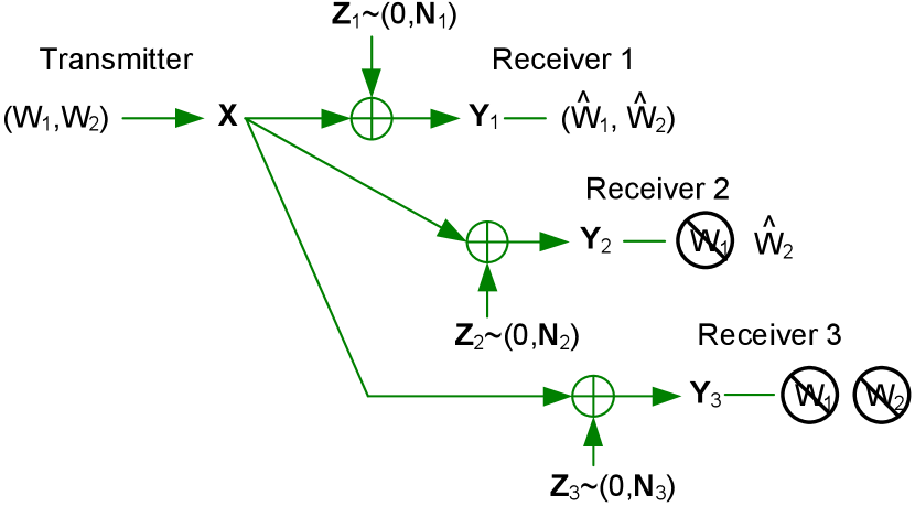
(a) Communication scenario 1

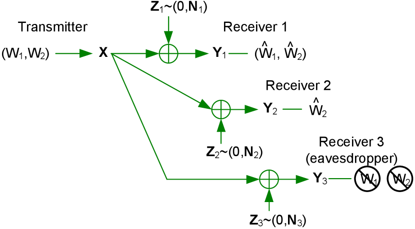
(b) Communication scenario 2

Figure 1: Degraded vector Gaussian broadcast channel with layered confidential messages

Consider the following vector Gaussian broadcast channel with three receivers:

$$\mathbf{Y}_{k}[t]=\mathbf{X}[t]+\mathbf{Z}_{k}[t],\quad k=1,2,3$$ (8)

where $\{\mathbf{Z}_{k}[t]\}_{t}$, $k=1,2,3$, are independent and identically distributed additive vector Gaussian noise processes with zero means and positive definite covariance matrices $\mathbf{N}_{k}$, respectively. The channel input $\{\mathbf{X}[t]\}_{t}$ is subject to a matrix constraint:

$$\frac{1}{n}\sum_{t=1}^{n}\mathbf{X}[t]\mathbf{X}^{\textsf{T}}[t]\preceq\mathbf{S}$$ (9)

where $\mathbf{S}$ is a positive semidefinite matrix, and $n$ is the block length. We assume that the noise covariance matrices are ordered as

$$\mathbf{N}_{1}\preceq\mathbf{N}_{2}\preceq\mathbf{N}_{3},$$ (10)

i.e., the received signal $\mathbf{Y}_{3}[t]$ is (stochastically) degraded with respect to $\mathbf{Y}_{2}[t]$, which is further degraded with respect to $\mathbf{Y}_{1}[t]$.

We consider two different communication scenarios, both with two independent messages $W_{1}$ and $W_{2}$. In the first scenario (see Fig. 1-(a)), message $W_{1}$ is intended for receiver 1 but needs to be kept secret from receivers 2 and 3, and message $W_{2}$ is intended for receivers 1 and 2 but needs to be kept confidential from receiver 3. In the second scenario (see Fig. 1-(b)), message $W_{1}$ is intended for receivers 1 but needs to be kept secret from receiver receiver 3, and message $W_{2}$ is intended for receivers 1 but needs to be kept secret from receiver 3. The confidentiality of the messages at the unintended receivers is measured using the normalized information-theoretic criteria [20, 21]:

$$\frac{1}{n}I(W_{1};\mathbf{Y}_{2}^{n})\rightarrow 0,\quad\frac{1}{n}I(W_{1};\mathbf{Y}_{3}^{n})\rightarrow 0,\quad\text{and}\quad\frac{1}{n}I(W_{2};\mathbf{Y}_{3}^{n})\rightarrow 0$$ (11)

for the first scenario and

$$\frac{1}{n}I(W_{1};\mathbf{Y}_{3}^{n})\rightarrow 0,\quad\text{and}\quad\frac{1}{n}I(W_{2};\mathbf{Y}_{3}^{n})\rightarrow 0$$ (12)

for the second scenario. Here, the limits are taken as the block length $n\rightarrow\infty$. The goal is to characterize the entire secrecy rate region $\mathcal{C}_{s}=\{(R_{1},R_{2})\}$ that can be achieved by any coding scheme.

To characterize the secrecy capacity regions, we will first consider the discrete memoryless version of the problem with transition probability $p(y_{1},y_{2},y_{3}|x)$ and degradedness order

$$X\rightarrow Y_{1}\rightarrow Y_{2}\rightarrow Y_{3}.$$ (13)

We have the following single-letter characterizations of the secrecy capacity regions.

Theorem 3

The secrecy capacity region of the discrete memoryless broadcast channel $p(y_{1},y_{2},y_{3}|x)$ with confidential messages $W_{1}$ (intended for receiver 1 but needs to be kept secret from receivers 2 and 3) and $W_{2}$ (intended for receivers 1 and 2 but needs to be kept secret from receiver 3) under the degradedness order (13) is given by the set of nonnegative rate pairs $(R_{1},R_{2})$ such that

$$R_{1}\leq \;I(X;Y_{1}|U)-I(X;Y_{2}|U)$$

and $$R_{2}\leq \;I(U;Y_{2})-I(U;Y_{3})$$ (14)

for some jointly distributed $(U,X)$ satisfying the Markov relation

$$U\rightarrow X\rightarrow(Y_{1},Y_{2},Y_{3}).$$

Theorem 4 ([22, Theorem 2])

The secrecy capacity region of the discrete memoryless broadcast channel $p(y_{1},y_{2},y_{3}|x)$ with confidential messages $W_{1}$ (intended for receiver 1 but needs to be kept secret from receiver 3) and $W_{2}$ (intended for receivers 1 and 2 but needs to be kept secret from receiver 3) under the degradedness order (13) is given by the set of nonnegative rate pairs $(R_{1},R_{2})$ such that

$$R_{1}\leq \;I(X;Y_{1}|U)-I(X;Y_{3}|U)$$

and $$R_{2}\leq \;I(U;Y_{2})-I(U;Y_{3})$$ (15)

for some jointly distributed $(U,X)$ satisfying the Markov relation

$$U\rightarrow X\rightarrow(Y_{1},Y_{2},Y_{3}).$$

A proof of Theorem 4 can be found in [22]. Theorem 3 can be proved in a similar fashion; for completeness, a proof is included in Appendix A. For the vector Gaussian broadcast channel (8) under the degradedness order (10), the single-letter expressions (14) and (15) can be further evaluated using the extremal entropy inequality (7). The results are summarized in the following theorems.

Theorem 5

The secrecy capacity region of the vector Gaussian broadcast channel (8) with confidential messages $W_{1}$ (intended for receiver 1 but needs to be kept secret from receivers 2 and 3) and $W_{2}$ (intended for receivers 1 and 2 but needs to be kept secret from receiver 3) and degradedness order (10) under the matrix constraint (9) is given by the set of nonnegative secrecy rate pairs $(R_{1},R_{2})$ such that

$$R_{1} \leq\;\frac{1}{2}\log\left|\frac{\mathbf{B}+\mathbf{N}_{1}}{\mathbf{N}_{1}}\right|-\frac{1}{2}\log\left|\frac{\mathbf{B}+\mathbf{N}_{2}}{\mathbf{N}_{2}}\right|$$

and $$R_{2} \leq\;\frac{1}{2}\log\left|\frac{\mathbf{S}+\mathbf{N}_{2}}{\mathbf{B}+\mathbf{N}_{2}}\right|-\frac{1}{2}\log\left|\frac{\mathbf{S}+\mathbf{N}_{3}}{\mathbf{B}+\mathbf{N}_{3}}\right|$$ (16)

for some $0\preceq\mathbf{B}\preceq\mathbf{S}$.

Theorem 6

The secrecy capacity region of the vector Gaussian broadcast channel (8) with confidential messages $W_{1}$ (intended for receiver 1 but needs to be kept secret from receiver 3) and $W_{2}$ (intended for receivers 1 and 2 but needs to be kept secret from receiver 3) and degradedness order (10) under the matrix constraint (9) is given by the set of nonnegative secrecy rate pairs $(R_{1},R_{2})$ such that

$$R_{1} \leq\;\frac{1}{2}\log\left|\frac{\mathbf{B}+\mathbf{N}_{1}}{\mathbf{N}_{1}}\right|-\frac{1}{2}\log\left|\frac{\mathbf{B}+\mathbf{N}_{3}}{\mathbf{N}_{3}}\right|$$

and $$R_{2} \leq\;\frac{1}{2}\log\left|\frac{\mathbf{S}+\mathbf{N}_{2}}{\mathbf{B}+\mathbf{N}_{2}}\right|-\frac{1}{2}\log\left|\frac{\mathbf{S}+\mathbf{N}_{3}}{\mathbf{B}+\mathbf{N}_{3}}\right|$$ (17)

for some $0\preceq\mathbf{B}\preceq\mathbf{S}$.

III Proof of Theorem 1

In this section, we prove the generalized Costa EPI (3) as stated in Theorem 1. We first examine the equality condition. Note that when $\mathbf{X}$ is Gaussian, the generalized Costa EPI (3) becomes the matrix inequality:

$$|\mathbf{B}+\mathbf{A}^{\frac{1}{2}}\mathbf{N}\mathbf{A}^{\frac{1}{2}}|^{\frac{1}{n}} \geq|\mathbf{B}-\mathbf{A}\mathbf{B}|^{\frac{1}{n}}+|\mathbf{A}\mathbf{B}+\mathbf{A}\mathbf{N}|^{\frac{1}{n}}.$$

Suppose that $\mathbf{B}-\mathbf{A}\mathbf{B}$ and $\mathbf{B}+\mathbf{A}^{\frac{1}{2}}\mathbf{N}\mathbf{A}^{\frac{1}{2}}$ are proportional, i.e., there exists a real scalar $c$ such that

$$\mathbf{B}+\mathbf{A}^{\frac{1}{2}}\mathbf{N}\mathbf{A}^{\frac{1}{2}}=c(\mathbf{B}-\mathbf{A}\mathbf{B}).$$

Since both matrices $\mathbf{A}$ and $\mathbf{B}$ are symmetric, this implies that $\mathbf{A}\mathbf{B}$ is also symmetric, i.e.,

$$\mathbf{A}\mathbf{B}=\mathbf{B}^{\textsf{T}}\mathbf{A}^{\textsf{T}}=\mathbf{B}\mathbf{A}.$$

Therefore, $\mathbf{A}$ and $\mathbf{B}$ must have the same eigenvector matrix [23] and hence

$$\mathbf{A}\mathbf{B} =\mathbf{A}^{\frac{1}{2}}\mathbf{B}\mathbf{A}^{\frac{1}{2}}.$$

It follows that

$$\mathbf{A}^{\frac{1}{2}}\mathbf{B}\mathbf{A}^{\frac{1}{2}}+\mathbf{A}^{\frac{1}{2}}\mathbf{N}\mathbf{A}^{\frac{1}{2}} =\mathbf{B}+\mathbf{A}^{\frac{1}{2}}\mathbf{N}\mathbf{A}^{\frac{1}{2}}-(\mathbf{B}-\mathbf{A}\mathbf{B})$$

$$=(c-1)(\mathbf{B}-\mathbf{A}\mathbf{B})$$

i.e., $\mathbf{A}^{\frac{1}{2}}\mathbf{B}\mathbf{A}^{\frac{1}{2}}+\mathbf{A}^{\frac{1}{2}}\mathbf{N}\mathbf{A}^{\frac{1}{2}}$ and $\mathbf{B}-\mathbf{A}\mathbf{B}$ are proportional. Therefore,

$$|\mathbf{B}+\mathbf{A}^{\frac{1}{2}}\mathbf{N}\mathbf{A}^{\frac{1}{2}}|^{\frac{1}{n}} =|\mathbf{B}-\mathbf{A}\mathbf{B}+(\mathbf{A}^{\frac{1}{2}}\mathbf{B}\mathbf{A}^{\frac{1}{2}}+\mathbf{A}^{\frac{1}{2}}\mathbf{N}\mathbf{A}^{\frac{1}{2}})|^{\frac{1}{n}}$$

$$=|\mathbf{B}-\mathbf{A}\mathbf{B}|^{\frac{1}{n}}+|\mathbf{A}^{\frac{1}{2}}\mathbf{B}\mathbf{A}^{\frac{1}{2}}+\mathbf{A}^{\frac{1}{2}}\mathbf{N}\mathbf{A}^{\frac{1}{2}}|^{\frac{1}{n}}$$

$$=|\mathbf{B}-\mathbf{A}\mathbf{B}|^{\frac{1}{n}}+|\mathbf{A}\mathbf{B}+\mathbf{A}\mathbf{N}|^{\frac{1}{n}}.$$

This proved the desired equality condition.

We now turn to the proof of the inequality. First consider the special case when $|\mathbf{A}|=0$. Since

$$h(\mathbf{X}+\mathbf{A}^{\frac{1}{2}}\mathbf{Z})-h(\mathbf{X})=I(\mathbf{A}^{\frac{1}{2}}\mathbf{Z};\mathbf{X}+\mathbf{A}^{\frac{1}{2}}\mathbf{Z})\geq 0,$$

we have

$$\exp\left[\frac{2}{n}h(\mathbf{X}+\mathbf{A}^{\frac{1}{2}}\mathbf{Z})\right] \geq\exp\left[\frac{2}{n}h(\mathbf{X})\right]$$

$$\geq|\mathbf{I}-\mathbf{A}|^{\frac{1}{n}}\exp\left[\frac{2}{n}h(\mathbf{X})\right]$$

where the last inequality follows from the assumption that $0\preceq\mathbf{A}\preceq\mathbf{I}$ and hence $0\leq|\mathbf{I}-\mathbf{A}|\leq 1$.

Next, consider the general case when $|\mathbf{A}|>0$. The proof is rather long so we divide it into several steps.

Step 1–Constructing a monotone path. To prove the generalized Costa EPI (3), we can equivalently show that

$$\exp\left[\frac{2}{n}h(\mathbf{X}+\mathbf{Z})\right] \leq|\mathbf{A}|^{-\frac{1}{n}}\exp\left[\frac{2}{n}h(\mathbf{X}+\mathbf{A}^{\frac{1}{2}}\mathbf{Z})\right]-\left(\frac{|\mathbf{I}-\mathbf{A}|}{|\mathbf{A}|}\right)^{\frac{1}{n}}\exp\left[\frac{2}{n}h(\mathbf{X})\right].$$ (18)

Since $\mathbf{X}$ and $\mathbf{Z}$ are independent, we have

$$h(\mathbf{X}+\mathbf{A}^{\frac{1}{2}}\mathbf{Z})-h(\mathbf{X}) =h(\mathbf{A}^{-\frac{1}{2}}\mathbf{X}+\mathbf{Z})-h(\mathbf{A}^{-\frac{1}{2}}\mathbf{X})$$

$$=h(\mathbf{A}^{-\frac{1}{2}}\mathbf{X}+\mathbf{Z})-h(\mathbf{A}^{-\frac{1}{2}}\mathbf{X}|\mathbf{Z})$$

$$=I(\mathbf{Z};\mathbf{A}^{-\frac{1}{2}}\mathbf{X}+\mathbf{Z})$$ (19)

and

$$h(\mathbf{X}+\mathbf{Z})-h(\mathbf{X})=I(\mathbf{Z};\mathbf{X}+\mathbf{Z}).$$ (20)

Divide both sides of (18) by $\exp\left[\frac{2}{n}h(\mathbf{X})\right]$ and use (19) and (20). Then, (18) can be equivalently written as

$$\exp\left[\frac{2}{n}I(\mathbf{Z};\mathbf{X}+\mathbf{Z})\right] \leq|\mathbf{A}|^{-\frac{1}{n}}\left\{\exp\left[\frac{2}{n}I(\mathbf{Z};\mathbf{A}^{-\frac{1}{2}}\mathbf{X}+\mathbf{Z})\right]-|\mathbf{I}-\mathbf{A}|^{\frac{1}{n}}\right\}.$$ (21)

Let

$$F(\mathbf{D}) :=|\mathbf{D}|^{\frac{2}{n}}\Biggl{\{}\exp\left[\frac{2}{n}I(\mathbf{Z};\mathbf{D}\mathbf{X}+\mathbf{Z})\right]-|\mathbf{I}-\mathbf{D}^{-2}|^{\frac{1}{n}}\Biggr{\}}.$$ (22)

With this definition, (21) can be equivalently written as

$$F(\mathbf{I})\leq F(\mathbf{A}^{-\frac{1}{2}}).$$ (23)

To show the inequality (23), it is sufficient to construct a family of $n\times n$ positive definite matrices $\{\mathbf{D}(\gamma)\}_{\gamma}$ connecting $\mathbf{I}$ and $\mathbf{A}^{-\frac{1}{2}}$ such that $F(\mathbf{D}(\gamma))$ is monotone along the path. Unlike the scalar case where there is only one path connecting $1$ to $1/\sqrt{a}$, in the matrix case there are infinitely many paths connecting $\mathbf{I}$ and $\mathbf{A}^{-\frac{1}{2}}$. Here, we consider the special choice

$$\mathbf{D}(\gamma):=\left[\mathbf{I}+\gamma(\mathbf{A}^{-1}-\mathbf{I})\right]^{\frac{1}{2}}$$ (24)

and show that

$$\frac{\partial F}{\partial\gamma}\geq 0,\quad\forall\gamma\in[0,1].$$ (25)

along this particular path.

Step 2–Calculating the derivative $\frac{\partial F}{\partial\gamma}$. Following [14, Theorem 5], we have

$$I(\mathbf{Z};\mathbf{D}\mathbf{X}+\mathbf{Z})=I(\mathbf{X};\mathbf{D}\mathbf{X}+\mathbf{Z})+h(\mathbf{Z})-h(\mathbf{X})-\log|\mathbf{D}|$$

and

$${\sf Cov}(\mathbf{X}|\mathbf{D}\mathbf{X}+\mathbf{Z})=\mathbf{D}^{-1}\,{\sf Cov}(\mathbf{Z}|\mathbf{D}\mathbf{X}+\mathbf{Z})\mathbf{D}^{-\textsf{T}}.$$

Let $\mathbf{N}:={\sf Cov}(\mathbf{Z})$ and note that $\mathbf{D}$ is symmetric. We have

$$\frac{\partial}{\partial\mathbf{D}}I(\mathbf{Z};\mathbf{D}\mathbf{X}+\mathbf{Z}) =\frac{\partial}{\partial\mathbf{D}}I(\mathbf{X};\mathbf{D}\mathbf{X}+\mathbf{Z})-\mathbf{D}^{-1}$$

$$=\mathbf{N}^{-1}\mathbf{D}\,{\sf Cov}(\mathbf{X}|\mathbf{D}\mathbf{X}+\mathbf{Z})-\mathbf{D}^{-1}$$

$$=\left(\mathbf{N}^{-1}{\sf Cov}(\mathbf{Z}|\mathbf{D}\mathbf{X}+\mathbf{Z})-\mathbf{I}\right)\mathbf{D}^{-1}$$ (26)

where the second equality follows from the fundamental relationship between the derivative of mutual information and MMSE estimate in linear vector Gaussian channels as stated in [18, Theorem 2].

From (26), the derivative $\frac{\partial F}{\partial\mathbf{D}}$ can be calculated as

$$\frac{\partial F}{\partial\mathbf{D}}= \frac{2}{n}|\mathbf{D}|^{\frac{2}{n}}\mathbf{D}^{-1}\Biggl{\{}\exp\left[\frac{2}{n}I(\mathbf{Z};\mathbf{D}\mathbf{X}+\mathbf{Z})\right]-|\mathbf{I}-\mathbf{D}^{-2}|^{\frac{1}{n}}\Bigg{\}}+$$

$$|\mathbf{D}|^{\frac{2}{n}}\Biggl{\{}\frac{2}{n}\exp\left[\frac{2}{n}I(\mathbf{Z};\mathbf{D}\mathbf{X}+\mathbf{Z})\right]\frac{\partial I(\mathbf{Z};\mathbf{D}\mathbf{X}+\mathbf{Z})}{\partial\mathbf{D}}-\frac{2}{n}|\mathbf{I}-\mathbf{D}^{-2}|^{\frac{1}{n}}(\mathbf{I}-\mathbf{D}^{-2})^{-1}\mathbf{D}^{-3}\Biggr{\}}$$

$$= \frac{2}{n}|\mathbf{D}|^{\frac{2}{n}}\Biggl{\{}\left\{\exp\left[\frac{2}{n}I(\mathbf{Z};\mathbf{D}\mathbf{X}+\mathbf{Z})\right]-|\mathbf{I}-\mathbf{D}^{-2}|^{\frac{1}{n}}\right\}\mathbf{I}+$$

$$\exp\left[\frac{2}{n}I(\mathbf{Z};\mathbf{D}\mathbf{X}+\mathbf{Z})\right](\mathbf{N}^{-1}{\sf Cov}(\mathbf{Z}|\mathbf{D}\mathbf{X}+\mathbf{Z})-\mathbf{I})-|\mathbf{I}-\mathbf{D}^{-2}|^{\frac{1}{n}}(\mathbf{D}^{2}-\mathbf{I})^{-1}\Biggr{\}}\mathbf{D}^{-1}$$

$$= \frac{2}{n}|\mathbf{D}|^{\frac{2}{n}}\Biggl{\{}\exp\left[\frac{2}{n}I(\mathbf{Z};\mathbf{D}\mathbf{X}+\mathbf{Z})\right]\mathbf{N}^{-1}{\sf Cov}(\mathbf{Z}|\mathbf{D}\mathbf{X}+\mathbf{Z})-|\mathbf{I}-\mathbf{D}^{-2}|^{\frac{1}{n}}\left[\mathbf{I}+(\mathbf{D}^{2}-\mathbf{I})^{-1}\right]\Biggr{\}}\mathbf{D}^{-1}.$$ (27)

The derivative $\frac{\partial\mathbf{D}}{\partial\gamma}$ can be calculated as

$$\frac{\partial\mathbf{D}}{\partial\gamma} =\frac{1}{2}\left[\mathbf{I}+\gamma(\mathbf{A}^{-1}-\mathbf{I})\right]^{-\frac{1}{2}}(\mathbf{A}^{-1}-\mathbf{I})$$

$$=\frac{1}{2\gamma}\mathbf{D}^{-1}(\mathbf{D}^{2}-\mathbf{I})$$

$$=\frac{1}{2\gamma}\mathbf{D}(\mathbf{I}-\mathbf{D}^{-2}).$$ (28)

By (27), (28) and the chain rule of differentiation [24, Chapter 17.5],

$$\frac{\partial F}{\partial\gamma} ={\sf Tr}\left\{\frac{\partial F}{\partial\mathbf{D}}\,\frac{\partial\mathbf{D}}{\partial\gamma}\right\}$$

$$=\frac{|\mathbf{D}|^{\frac{2}{n}}}{n}{\sf Tr}\Biggl{\{}\left[\exp\left[\frac{2}{n}I(\mathbf{Z};\mathbf{D}\mathbf{X}+\mathbf{Z})\right]\mathbf{N}^{-1}{\sf Cov}(\mathbf{Z}|\mathbf{D}\mathbf{X}+\mathbf{Z})-|\mathbf{I}-\mathbf{D}^{-2}|^{\frac{1}{n}}\left[\mathbf{I}+(\mathbf{D}^{2}-\mathbf{I})^{-1}\right]\right]\frac{\mathbf{I}-\mathbf{D}^{-2}}{\gamma}\Biggr{\}}$$

$$=\frac{|\mathbf{D}|^{\frac{2}{n}}}{n\gamma}{\sf Tr}\left\{\exp\left[\frac{2}{n}I(\mathbf{Z};\mathbf{D}\mathbf{X}+\mathbf{Z})\right]\mathbf{N}^{-1}{\sf Cov}(\mathbf{Z}|\mathbf{D}\mathbf{X}+\mathbf{Z})(\mathbf{I}-\mathbf{D}^{-2})-|\mathbf{I}-\mathbf{D}^{-2}|^{\frac{1}{n}}\mathbf{I}\right\}$$

$$=\frac{|\mathbf{D}|^{\frac{2}{n}}}{n\gamma}\left\{\exp\left[\frac{2}{n}I(\mathbf{Z};\mathbf{D}\mathbf{X}+\mathbf{Z})\right]{\sf Tr}\left\{\mathbf{N}^{-1}{\sf Cov}(\mathbf{Z}|\mathbf{D}\mathbf{X}+\mathbf{Z})(\mathbf{I}-\mathbf{D}^{-2})\right\}-n|\mathbf{I}-\mathbf{D}^{-2}|^{\frac{1}{n}}\right\}.$$ (29)

Step 3–Proving $\frac{\partial F}{\partial\gamma}\geq 0$. The mutual information $I(\mathbf{Z};\mathbf{D}\mathbf{X}+\mathbf{Z})$ can be bounded from below as follows:

$$I(\mathbf{Z};\mathbf{D}\mathbf{X}+\mathbf{Z}) \geq I(\mathbf{Z};{\sf E}[\mathbf{Z}|\mathbf{D}\mathbf{X}+\mathbf{Z}])$$

$$=h(\mathbf{Z})-h(\mathbf{Z}|{\sf E}[\mathbf{Z}|\mathbf{D}\mathbf{X}+\mathbf{Z}])$$

$$=\frac{1}{2}\log(2\pi e)^{n}|\mathbf{N}|-h(\mathbf{Z}-{\sf E}[\mathbf{Z}|\mathbf{D}\mathbf{X}+\mathbf{Z}]|{\sf E}[\mathbf{Z}|\mathbf{D}\mathbf{X}+\mathbf{Z}])$$

$$\geq\frac{1}{2}\log(2\pi e)^{n}|\mathbf{N}|-h(\mathbf{Z}-{\sf E}[\mathbf{Z}|\mathbf{D}\mathbf{X}+\mathbf{Z}])$$

$$\geq\frac{1}{2}\log(2\pi e)^{n}|\mathbf{N}|-\frac{1}{2}\log(2\pi e)^{n}\bigl{|}{\sf Cov}(\mathbf{Z}|\mathbf{D}\mathbf{X}+\mathbf{Z})\bigr{|}$$

$$=\frac{1}{2}\log\frac{|\mathbf{N}|}{|{\sf Cov}(\mathbf{Z}|\mathbf{D}\mathbf{X}+\mathbf{Z})|}.$$ (30)

Here, the first inequality follows from the Markov relation

$$\mathbf{Z}\rightarrow\mathbf{D}\mathbf{X}+\mathbf{Z}\rightarrow{\sf E}[\mathbf{Z}|\mathbf{D}\mathbf{X}+\mathbf{Z}]$$

and the chain rule of mutual information [25, Chapter 2.8]; the second inequality follows from the fact that conditioning reduces differential entropy [25, Chapter 9.6]; and the third inequality follows from the well-known fact that Gaussian maximizes differential entropy for a given covariance matrix [25, Chapter 9.6]. By (30),

$$|\mathbf{I}-\mathbf{D}^{-2}|^{\frac{1}{n}}\exp\left[-\frac{2}{n}I(\mathbf{Z};\mathbf{D}\mathbf{X}+\mathbf{Z})\right] \leq\;|\mathbf{N}^{-1}{\sf Cov}(\mathbf{Z}|\mathbf{D}\mathbf{X}+\mathbf{Z})(\mathbf{I}-\mathbf{D}^{-2})|^{\frac{1}{n}}$$

$$\leq\;\frac{1}{n}{\sf Tr}\left\{\mathbf{N}^{-1}{\sf Cov}(\mathbf{Z}|\mathbf{D}\mathbf{X}+\mathbf{Z})(\mathbf{I}-\mathbf{D}^{-2})\right\}$$ (31)

where the last inequality follows from the well-known inequality of arithmetic and geometric means [26, p. 136].

Finally, substituting (31) into (29) establishes the fact that $\frac{\partial F}{\partial\gamma}\geq 0$ for all $\gamma\in[0,1]$. In particular, we have $F(\mathbf{D}(1))\geq F(\mathbf{D}(0))$. This proved the desired inequality (21) and hence the generalized Costa EPI (3).

IV Proof of Theorem 2

In this section, we prove the extremal entropy inequality (7) as stated in Theorem 2. We will first state a series of corollaries of Theorem 1, as intermediate results leading to Theorem 2. Based on the final corollary, we will prove Theorem 2 using an enhancement argument.

Corollary 1

Let $\mathbf{Z}$ be a Gaussian random $n$-vector with a positive definite covariance matrix, and let $\mathbf{A}$ be an $n\times n$ positive real symmetric matrix such that $0\preceq\mathbf{A}\preceq\mathbf{I}$. Then

$$\exp\left[\frac{2}{n}h(\mathbf{X}+\mathbf{A}^{\frac{1}{2}}\mathbf{Z}|U)\right] \geq|\mathbf{I}-\mathbf{A}|^{\frac{1}{n}}\exp\left[\frac{2}{n}h(\mathbf{X}|U)\right]+|\mathbf{A}|^{\frac{1}{n}}\exp\left[\frac{2}{n}h(\mathbf{X}+\mathbf{Z}|U)\right]$$ (32)

for any $(\mathbf{X},U)$ independent of $\mathbf{Z}$.

Corollary 2

Let $\mathbf{Z}_{1}$, $\mathbf{Z}_{2}$ and $\mathbf{Z}_{3}$ be Gaussian random $n$-vectors with positive definite covariance matrices $\mathbf{N}_{1}$, $\mathbf{N}_{2}$ and $\mathbf{N}_{3}$, respectively. Assume that $\mathbf{N}_{1}\preceq\mathbf{N}_{3}$. If there exists an $n\times n$ positive semidefinite matrix $\mathbf{B}^{*}$ such that

$$(\mathbf{B}^{*}+\mathbf{N}_{1})^{-1}+\mu(\mathbf{B}^{*}+\mathbf{N}_{3})^{-1}=(1+\mu)(\mathbf{B}^{*}+\mathbf{N}_{2})^{-1}$$ (33)

for some real scalar $\mu\geq 0$, then

$$h(\mathbf{X}+\mathbf{Z}_{1}|U)+\mu h (\mathbf{X}+\mathbf{Z}_{3}|U)-(1+\mu)h(\mathbf{X}+\mathbf{Z}_{2}|U)$$

$$\leq\frac{1}{2}\log|\mathbf{B}^{*}+\mathbf{N}_{1}|+\frac{\mu}{2}\log|\mathbf{B}^{*}+\mathbf{N}_{3}|-\frac{1+\mu}{2}\log|\mathbf{B}^{*}+\mathbf{N}_{2}|$$ (34)

for any $(\mathbf{X},U)$ independent of $(\mathbf{Z}_{1},\mathbf{Z}_{2},\mathbf{Z}_{3})$.

Corollary 3

Let $\mathbf{Z}_{k}$, $k=0,\ldots,K$, be a collection of $K+1$ Gaussian random $n$-vectors with respective positive definite covariance matrices $\mathbf{N}_{k}$. Assume that $\mathbf{N}_{1}\preceq\ldots\preceq\mathbf{N}_{K}$. If there exists an $n\times n$ positive semidefinite matrix $\mathbf{B}^{*}$ such that

$$\sum_{k=1}^{K}\mu_{k}(\mathbf{B}^{*}+\mathbf{N}_{k})^{-1}=(\mathbf{B}^{*}+\mathbf{N}_{0})^{-1}$$ (35)

for some $\mu_{k}\geq 0$ with $\sum_{k=1}^{K}\mu_{k}=1$, then

$$\sum_{k=1}^{K}\mu_{k}h(\mathbf{X}+\mathbf{Z}_{k}|U)-h(\mathbf{X}+\mathbf{Z}_{0}|U) \leq\sum_{k=1}^{K}\frac{\mu_{k}}{2}\log|\mathbf{B}^{*}+\mathbf{N}_{k}|-\frac{1}{2}\log|\mathbf{B}^{*}+\mathbf{N}_{0}|$$ (36)

for any $(\mathbf{X},U)$ independent of $(\mathbf{Z}_{0},\ldots,\mathbf{Z}_{K})$.

A proof of Corollaries 1, 2 and 3 can be found in Appendices B, C and D, respectively. We are now ready to prove Theorem 2. Note that the special case with $\mathbf{M}_{1}=\mathbf{M}_{2}=0$ was proved in Corollary 3. To extend the result of Corollary 3 to nonzero $\mathbf{M}_{1}$ and $\mathbf{M}_{2}$, we will consider an enhancement argument, which was first introduced by Weingarten, Steinberg and Shamai in [7].

Let $\widetilde{\mathbf{N}}_{1}$ and $\widetilde{\mathbf{N}}_{0}$ be $n\times n$ real symmetric matrices such that:

$$\mu_{1}(\mathbf{B}^{*}+\widetilde{\mathbf{N}}_{1})^{-1} =\mu_{1}(\mathbf{B}^{*}+\mathbf{N}_{1})^{-1}+\mathbf{M}_{1}$$ (37)

$$\mbox{and}\quad\quad(\mathbf{B}^{*}+\widetilde{\mathbf{N}}_{0})^{-1} =(\mathbf{B}^{*}+\mathbf{N}_{0})^{-1}+\mathbf{M}_{2}.$$ (38)

As shown in [7, Lemma 11 and 12], $\widetilde{\mathbf{N}}_{1}$ and $\widetilde{\mathbf{N}}_{0}$ satisfy the following properties:

$$0\prec\widetilde{\mathbf{N}}_{1} =\left(\mathbf{N}_{1}^{-1}+\mu_{1}^{-1}\mathbf{M}_{1}\right)^{-1}\preceq\mathbf{N}_{1},$$ (39)

$$\widetilde{\mathbf{N}}_{1} \preceq\widetilde{\mathbf{N}}_{0}\preceq\mathbf{N}_{0},$$ (40)

$$\left|\frac{\mathbf{B}^{*}+\widetilde{\mathbf{N}}_{1}}{\widetilde{\mathbf{N}}_{1}}\right| =\left|\frac{\mathbf{B}^{*}+\mathbf{N}_{1}}{\mathbf{N}_{1}}\right|$$ (41)

and

$$\left|\frac{\mathbf{S}+\widetilde{\mathbf{N}}_{0}}{\mathbf{B}^{*}+\widetilde{\mathbf{N}}_{0}}\right| =\left|\frac{\mathbf{S}+\mathbf{N}_{2}}{\mathbf{B}^{*}+\mathbf{N}_{2}}\right|.$$ (42)

Let $\widetilde{\mathbf{Z}}_{0}$ and $\widetilde{\mathbf{Z}}_{1}$ be two Gaussian $n$-vectors with covariance matrices $\widetilde{\mathbf{N}}_{0}$ and $\widetilde{\mathbf{N}}_{1}$, respectively. Note from (39) that $\widetilde{\mathbf{N}}_{1}\preceq\mathbf{N}_{1}\preceq\mathbf{N}_{2}\preceq\ldots\preceq\mathbf{N}_{K}$. Moreover, substitute (37) and (38) into (4) and we have

$$\mu_{1}(\mathbf{B}^{*}+\widetilde{\mathbf{N}}_{1})^{-1}+\sum_{k=2}^{K}\mu_{k}(\mathbf{B}^{*}+\mathbf{N}_{k})^{-1} =(\mathbf{B}^{*}+\widetilde{\mathbf{N}}_{0})^{-1}.$$ (43)

Thus, by Corollary 3

$$\mu_{1}h(\mathbf{X}+\widetilde{\mathbf{Z}}_{1}|U)+ \sum_{k=2}^{K}\mu_{k}h(\mathbf{X}+\mathbf{Z}_{k}|U)-h(\mathbf{X}+\widetilde{\mathbf{Z}}_{0}|U)$$

$$\leq\frac{\mu_{1}}{2}(\mathbf{B}^{*}+\widetilde{\mathbf{N}}_{1})^{-1}+\sum_{k=2}^{K}\frac{\mu_{k}}{2}\log|\mathbf{B}^{*}+\mathbf{N}_{k}|-\frac{1}{2}\log|\mathbf{B}^{*}+\widetilde{\mathbf{N}}_{0}|$$ (44)

for any $(\mathbf{X},U)$ independent of $(\widetilde{\mathbf{Z}}_{0},\widetilde{\mathbf{Z}}_{1},\mathbf{Z}_{2},\ldots,\mathbf{Z}_{K})$.

On the other hand, note from (39) that $\widetilde{\mathbf{N}}_{1}\preceq\mathbf{N}_{1}$. We have

$$I(\mathbf{X};\mathbf{X}+\mathbf{Z}_{1}|U)\leq I(\mathbf{X};\mathbf{X}+\widetilde{\mathbf{Z}}_{1}|U)$$

for any $(\mathbf{X},U)$ independent of $(\mathbf{Z}_{1},\widetilde{\mathbf{Z}}_{1})$. Thus,

$$h(\mathbf{X}+\widetilde{\mathbf{Z}}_{1}|U)-h(\mathbf{X}+\mathbf{Z}_{1}|U) \geq h(\widetilde{\mathbf{Z}}_{1})-h(\mathbf{Z}_{1})$$

$$=\frac{1}{2}\log\left|\frac{\widetilde{\mathbf{N}}_{1}}{\mathbf{N}_{1}}\right|$$

$$=\frac{1}{2}\log\left|\frac{\mathbf{B}^{*}+\widetilde{\mathbf{N}}_{1}}{\mathbf{B}^{*}+\mathbf{N}_{1}}\right|$$ (45)

where the last equality follows from (41).

Also note from (40) that $\widetilde{\mathbf{N}}_{0}\preceq\mathbf{N}_{0}$. Let $\hat{\mathbf{Z}}_{0}$ be a Gaussian $n$-vector with covariance matrix $\mathbf{N}_{0}-\widetilde{\mathbf{N}}_{0}$ and independent of $(\widetilde{\mathbf{Z}}_{0},\mathbf{X},U)$. We have

$$h(\mathbf{X}+\mathbf{Z}_{0}|U)-h(\mathbf{X}+\widetilde{\mathbf{Z}}_{0}|U) =h(\mathbf{X}+\widetilde{\mathbf{Z}}_{0}+\hat{\mathbf{Z}}_{0}|U)-h(\mathbf{X}+\widetilde{\mathbf{Z}}_{0}|U)$$

$$=I(\hat{\mathbf{Z}}_{0};\mathbf{X}+\widetilde{\mathbf{Z}}_{0}+\hat{\mathbf{Z}}_{0}|U)$$

$$\geq I(\hat{\mathbf{Z}}_{0};\mathbf{X}+\widetilde{\mathbf{Z}}_{0}+\hat{\mathbf{Z}}_{0})$$

$$\geq\frac{1}{2}\log\left|\frac{{\sf Cov}(\mathbf{X})+\mathbf{N}_{0}}{{\sf Cov}(\mathbf{X})+\widetilde{\mathbf{N}}_{0}}\right|$$

$$\geq\frac{1}{2}\log\left|\frac{\mathbf{S}+\mathbf{N}_{0}}{\mathbf{S}+\widetilde{\mathbf{N}}_{0}}\right|$$ (46)

$$=\frac{1}{2}\log\left|\frac{\mathbf{B}^{*}+\mathbf{N}_{0}}{\mathbf{B}^{*}+\widetilde{\mathbf{N}}_{0}}\right|$$ (47)

for any $(\mathbf{X},U)$ independent of $(\mathbf{Z}_{0},\widetilde{\mathbf{Z}}_{0})$ such that ${\sf E}[\mathbf{X}\mathbf{X}^{\textsf{T}}]\preceq\mathbf{S}$. Here, the first inequality follows from the independence of $\hat{\mathbf{Z}}_{0}$ and $U$; the second inequality follows from the worst noise result [27, Lemma II.2]; the third inequality follows from the fact that $\widetilde{\mathbf{N}}_{0}\preceq\mathbf{N}_{0}$ and ${\sf Cov}(\mathbf{X})\preceq{\sf E}[\mathbf{X}\mathbf{X}^{\textsf{T}}]\preceq\mathbf{S}$; and the last inequality follows from (42).

Finally, put together (44), (45) and (47) and we may obtain

$$\sum_{k=1}^{K}\mu_{k} h(\mathbf{X}+\mathbf{Z}_{k}|U)-h(\mathbf{X}+\mathbf{Z}_{0}|U)$$

$$=\left[\mu_{1}h(\mathbf{X}+\widetilde{\mathbf{Z}}_{1}|U)+\sum_{k=2}^{K}\mu_{k}h(\mathbf{X}+\mathbf{Z}_{k}|U)-h(\mathbf{X}+\widetilde{\mathbf{Z}}_{0}|U)\right]-$$

$$\hskip 16.0pt\mu_{1}\left[h(\mathbf{X}+\widetilde{\mathbf{Z}}_{1}|U)-h(\mathbf{X}+\mathbf{Z}_{1}|U)\right]-\left[h(\mathbf{X}+\mathbf{Z}_{0}|U)-h(\mathbf{X}+\widetilde{\mathbf{Z}}_{0}|U)\right]$$

$$\leq\left[\frac{\mu_{1}}{2}(\mathbf{B}^{*}+\widetilde{\mathbf{N}}_{1})^{-1}+\sum_{k=2}^{K}\frac{\mu_{k}}{2}\log|\mathbf{B}^{*}+\mathbf{N}_{k}|-\frac{1}{2}\log|\mathbf{B}^{*}+\widetilde{\mathbf{N}}_{0}|\right]-$$

$$\hskip 16.0pt\frac{\mu_{1}}{2}\log\left|\frac{\mathbf{B}^{*}+\widetilde{\mathbf{N}}_{1}}{\mathbf{B}^{*}+\mathbf{N}_{1}}\right|-\frac{1}{2}\log\left|\frac{\mathbf{B}^{*}+\mathbf{N}_{0}}{\mathbf{B}^{*}+\widetilde{\mathbf{N}}_{0}}\right|$$

$$=\sum_{k=1}^{K}\frac{\mu_{k}}{2}\log|\mathbf{B}^{*}+\mathbf{N}_{k}|-\frac{1}{2}\log|\mathbf{B}^{*}+\mathbf{N}_{0}|$$

for any $(\mathbf{X},U)$ independent of $(\mathbf{Z}_{0},\mathbf{Z}_{1},\ldots,\mathbf{Z}_{K})$ such that ${\sf E}[\mathbf{X}\mathbf{X}^{\textsf{T}}]\preceq\mathbf{S}$. This completes the proof of Theorem 2.

V Proof of Theorem 5

In this section, we prove Theorem 5. Note that the achievability of the secrecy rate region (16) can be obtained from the secrecy rate region (14) by letting $\mathbf{U}$ and $\mathbf{V}$ be two independent Gaussian vectors with zero means and covariance matrices $\mathbf{S}-\mathbf{B}$ and $\mathbf{B}$, respectively and $\mathbf{X}=\mathbf{U}+\mathbf{V}$. We therefore concentrate on the converse part of the theorem.

To show that (16) is indeed the secrecy capacity region of the vector Gaussian broadcast channel (8), we will consider proof by contradiction. Assume that $(R_{1}^{o},R_{2}^{o})$ is an achievable secrecy rate pair that lies outside the secrecy rate region (16). Note that $\mathbf{N}_{1}\preceq\mathbf{N}_{2}$. From [28, Theorem 1], we can bound $R_{1}^{o}$ by

$$R_{1}^{o}\leq\frac{1}{2}\log\left|\frac{\mathbf{S}+\mathbf{N}_{1}}{\mathbf{N}_{1}}\right|-\frac{1}{2}\log\left|\frac{\mathbf{S}+\mathbf{N}_{2}}{\mathbf{N}_{2}}\right|=R_{1}^{max}.$$

Note that when $R_{2}^{o}=0$, $R_{1}^{max}$ is achievable by letting $\mathbf{B}=\mathbf{S}$ in (14). Thus, we may assume that $R_{2}^{o}>0$ and write $R_{1}^{o}=R_{1}^{*}+\delta$ for some $\delta>0$ where $R_{1}^{*}$ is given by

$$\max_{\mathbf{B}} \quad\left[\frac{1}{2}\log\left|\frac{\mathbf{B}+\mathbf{N}_{1}}{\mathbf{N}_{1}}\right|-\frac{1}{2}\log\left|\frac{\mathbf{B}+\mathbf{N}_{2}}{\mathbf{N}_{2}}\right|\right]$$

subject to: $$\quad 0\preceq\mathbf{B}\preceq\mathbf{S}$$

$$\quad\frac{1}{2}\log\left|\frac{\mathbf{S}+\mathbf{N}_{2}}{\mathbf{B}+\mathbf{N}_{2}}\right|-\frac{1}{2}\log\left|\frac{\mathbf{S}+\mathbf{N}_{3}}{\mathbf{B}+\mathbf{N}_{3}}\right|\geq R_{2}^{o}.$$

Let $\mathbf{B}^{*}$ be an optimal solution to the above optimization program. Then, $\mathbf{B}^{*}$ must satisfy the following KKT conditions:

$$(\mathbf{B}^{*}+\mathbf{N}_{1})^{-1}+\mu(\mathbf{B}^{*}+\mathbf{N}_{3})^{-1}+\mathbf{M}_{1} =(1+\mu)(\mathbf{B}^{*}+\mathbf{N}_{2})^{-1}+\mathbf{M}_{2}$$ (48)

$$\mathbf{B}^{*}\mathbf{M}_{1} =0$$ (49)

$$\mbox{and}\quad\quad(\mathbf{S}-\mathbf{B}^{*})\mathbf{M}_{2} =0$$ (50)

where $\mathbf{M}_{1}$ and $\mathbf{M}_{2}$ are $n\times n$ positive semidefinite matrices, and $\mu$ is a nonnegative real scalar such that $\mu>0$ if and only if

$$\frac{1}{2}\log\left|\frac{\mathbf{S}+\mathbf{N}_{2}}{\mathbf{B}^{*}+\mathbf{N}_{2}}\right|-\frac{1}{2}\log\left|\frac{\mathbf{S}+\mathbf{N}_{3}}{\mathbf{B}^{*}+\mathbf{N}_{3}}\right|=R_{2}^{o}.$$

Thus,

$$R_{1}^{o}+\mu R_{2}^{o}=\left[\frac{1}{2}\log\left|\frac{\mathbf{B}^{*}+\mathbf{N}_{1}}{\mathbf{N}_{1}}\right|-\frac{1}{2}\log\left|\frac{\mathbf{B}^{*}+\mathbf{N}_{2}}{\mathbf{N}_{2}}\right|\right]+\mu\left[\frac{1}{2}\log\left|\frac{\mathbf{S}+\mathbf{N}_{2}}{\mathbf{B}^{*}+\mathbf{N}_{2}}\right|-\frac{1}{2}\log\left|\frac{\mathbf{S}+\mathbf{N}_{3}}{\mathbf{B}^{*}+\mathbf{N}_{3}}\right|\right]+\delta.$$ (51)

On the other hand, by the converse part of Theorem 3

$$R_{1}^{o}+\mu R_{2}^{o}\leq\; [I(\mathbf{X};\mathbf{X}+\mathbf{Z}_{1}|U)-I(\mathbf{X};\mathbf{X}+\mathbf{Z}_{2}|U)]+\mu[I(U;\mathbf{X}+\mathbf{Z}_{2})-I(U;\mathbf{X}+\mathbf{Z}_{3})]$$

$$=\; [h(\mathbf{Z}_{2})-h(\mathbf{Z}_{1})]-\mu[h(\mathbf{X}+\mathbf{Z}_{3})-h(\mathbf{X}+\mathbf{Z}_{2})]+$$

$$[h(\mathbf{X}+\mathbf{Z}_{1}|U)+\mu h(\mathbf{X}+\mathbf{Z}_{3}|U)-(1+\mu)h(\mathbf{X}+\mathbf{Z}_{2}|U)]$$

$$=\; \frac{1}{2}\log\left|\frac{\mathbf{N}_{2}}{\mathbf{N}_{1}}\right|-\mu[h(\mathbf{X}+\mathbf{Z}_{3})-h(\mathbf{X}+\mathbf{Z}_{2})]+$$

$$[h(\mathbf{X}+\mathbf{Z}_{1}|U)+\mu h(\mathbf{X}+\mathbf{Z}_{3}|U)-(1+\mu)h(\mathbf{X}+\mathbf{Z}_{2}|U)]$$ (52)

for some jointly distributed $(U,\mathbf{X})$ independent of $(\mathbf{Z}_{1},\mathbf{Z}_{2},\mathbf{Z}_{3})$. Note that $\mathbf{N}_{2}\preceq\mathbf{N}_{3}$. Similar to (46), we may obtain

$$h(\mathbf{X}+\mathbf{Z}_{3})-h(\mathbf{X}+\mathbf{Z}_{2}) \geq\frac{1}{2}\log\left|\frac{\mathbf{S}+\mathbf{N}_{3}}{\mathbf{S}+\mathbf{N}_{2}}\right|.$$ (53)

Moreover, by letting

$$\mu_{1}=\frac{1}{1+\mu},\quad\mu_{3}=\frac{\mu}{1+\mu},\quad\tilde{\mathbf{M}}_{1}=\frac{\mathbf{M}_{1}}{1+\mu},\quad\mbox{and}\;\;\tilde{\mathbf{M}}_{2}=\frac{\mathbf{M}_{2}}{1+\mu}$$

we can rewrite the KKT conditions (48)–(50) as

$$\mu_{1}(\mathbf{B}^{*}+\mathbf{N}_{1})^{-1}+\mu_{3}(\mathbf{B}^{*}+\mathbf{N}_{3})^{-1}+\tilde{\mathbf{M}}_{1} =(\mathbf{B}^{*}+\mathbf{N}_{2})^{-1}+\tilde{\mathbf{M}}_{2}$$

$$\mathbf{B}^{*}\tilde{\mathbf{M}}_{1} =0$$

$$\mbox{and}\quad\quad(\mathbf{S}-\mathbf{B}^{*})\tilde{\mathbf{M}}_{2} =0.$$

Thus, by Theorem 2

$$h(\mathbf{X}+\mathbf{Z}_{1}|U)+\mu h (\mathbf{X}+\mathbf{Z}_{3}|U)-(1+\mu)h(\mathbf{X}+\mathbf{Z}_{2}|U)$$

$$\leq\frac{1}{2}\log|\mathbf{B}^{*}+\mathbf{N}_{1}|+\frac{\mu}{2}\log|\mathbf{B}^{*}+\mathbf{N}_{3}|-\frac{1+\mu}{2}\log|\mathbf{B}^{*}+\mathbf{N}_{2}|.$$ (54)

Substituting (53) and (54) into (52), we have

$$R_{1}^{o}+\mu R_{2}^{o}\leq \;\frac{1}{2}\log\left|\frac{\mathbf{N}_{2}}{\mathbf{N}_{1}}\right|-\frac{\mu}{2}\log\left|\frac{\mathbf{S}+\mathbf{N}_{3}}{\mathbf{S}+\mathbf{N}_{2}}\right|+$$

$$\;\left[\frac{1}{2}\log|\mathbf{B}^{*}+\mathbf{N}_{1}|+\frac{\mu}{2}\log|\mathbf{B}^{*}+\mathbf{N}_{3}|-\frac{1+\mu}{2}\log|\mathbf{B}^{*}+\mathbf{N}_{2}|\right]$$

$$= \;\left[\frac{1}{2}\log\left|\frac{\mathbf{B}^{*}+\mathbf{N}_{1}}{\mathbf{N}_{1}}\right|-\frac{1}{2}\log\left|\frac{\mathbf{B}^{*}+\mathbf{N}_{2}}{\mathbf{N}_{2}}\right|\right]+\mu\left[\frac{1}{2}\log\left|\frac{\mathbf{S}+\mathbf{N}_{2}}{\mathbf{B}^{*}+\mathbf{N}_{2}}\right|-\frac{1}{2}\log\left|\frac{\mathbf{S}+\mathbf{N}_{3}}{\mathbf{B}^{*}+\mathbf{N}_{3}}\right|\right].$$ (55)

Thus, we have obtained a contradiction between (51) and (55). As a result, all the achievable rate pairs must be inside the secrecy rate region (16). This completes the proof of the theorem.

VI Proof of Theorem 6

In this section, we prove Theorem 6 following similar steps as those used in the proof for Theorem 5. The achievability of the secrecy rate region (17) can be obtained from the secrecy rate region (15) by letting $\mathbf{U}$ and $\mathbf{V}$ be two independent Gaussian vectors with zero means and covariance matrices $\mathbf{S}-\mathbf{B}$ and $\mathbf{B}$, respectively and $\mathbf{X}=\mathbf{U}+\mathbf{V}$. We therefore concentrate on the converse part of the theorem.

To show that (17) is indeed the secrecy capacity region of the vector Gaussian broadcast channel (8), we will use proof by contradiction. Assume that $(R_{1}^{o},R_{2}^{o})$ is an achievable secrecy rate pair that lies outside the secrecy rate region (17). Note that $\mathbf{N}_{1}\preceq\mathbf{N}_{3}$. From [28, Theorem 1], we can bound $R_{1}^{o}$ by

$$R_{1}^{o}\leq\frac{1}{2}\log\left|\frac{\mathbf{S}+\mathbf{N}_{1}}{\mathbf{N}_{1}}\right|-\frac{1}{2}\log\left|\frac{\mathbf{S}+\mathbf{N}_{3}}{\mathbf{N}_{3}}\right|=R_{1}^{max}.$$

Note that when $R_{2}^{o}=0$, $R_{1}^{max}$ is achievable by letting $\mathbf{B}=\mathbf{S}$ in (15). Thus, we may assume that $R_{2}^{o}>0$ and write $R_{1}^{o}=R_{1}^{*}+\delta$ for some $\delta>0$ where $R_{1}^{*}$ is given by

$$\max_{\mathbf{B}} \quad\left[\frac{1}{2}\log\left|\frac{\mathbf{B}+\mathbf{N}_{1}}{\mathbf{N}_{1}}\right|-\frac{1}{2}\log\left|\frac{\mathbf{B}+\mathbf{N}_{3}}{\mathbf{N}_{3}}\right|\right]$$

subject to: $$\quad 0\preceq\mathbf{B}\preceq\mathbf{S}$$

$$\quad\frac{1}{2}\log\left|\frac{\mathbf{S}+\mathbf{N}_{2}}{\mathbf{B}+\mathbf{N}_{2}}\right|-\frac{1}{2}\log\left|\frac{\mathbf{S}+\mathbf{N}_{3}}{\mathbf{B}+\mathbf{N}_{3}}\right|\geq R_{2}^{o}.$$

Let $\mathbf{B}^{*}$ be an optimal solution to the above optimization program. Then, $\mathbf{B}^{*}$ must satisfy the following KKT conditions:

$$(\mathbf{B}^{*}+\mathbf{N}_{1})^{-1}+(\mu-1)(\mathbf{B}^{*}+\mathbf{N}_{3})^{-1}+\mathbf{M}_{1} =\mu(\mathbf{B}^{*}+\mathbf{N}_{2})^{-1}+\mathbf{M}_{2}$$ (56)

$$\mathbf{B}^{*}\mathbf{M}_{1} =0$$ (57)

$$\mbox{and}\quad\quad(\mathbf{S}-\mathbf{B}^{*})\mathbf{M}_{2} =0$$ (58)

where $\mathbf{M}_{1}$ and $\mathbf{M}_{2}$ are $n\times n$ positive semidefinite matrices, and $\mu$ is a nonnegative real scalar such that $\mu\geq 1$. Therefore,

$$R_{2}^{o}=\frac{1}{2}\log\left|\frac{\mathbf{S}+\mathbf{N}_{2}}{\mathbf{B}^{*}+\mathbf{N}_{2}}\right|-\frac{1}{2}\log\left|\frac{\mathbf{S}+\mathbf{N}_{3}}{\mathbf{B}^{*}+\mathbf{N}_{3}}\right|$$

and

$$R_{1}^{o}+\mu R_{2}^{o}=\left[\frac{1}{2}\log\left|\frac{\mathbf{B}^{*}+\mathbf{N}_{1}}{\mathbf{N}_{1}}\right|-\frac{1}{2}\log\left|\frac{\mathbf{B}^{*}+\mathbf{N}_{3}}{\mathbf{N}_{3}}\right|\right]+\mu\left[\frac{1}{2}\log\left|\frac{\mathbf{S}+\mathbf{N}_{2}}{\mathbf{B}^{*}+\mathbf{N}_{2}}\right|-\frac{1}{2}\log\left|\frac{\mathbf{S}+\mathbf{N}_{3}}{\mathbf{B}^{*}+\mathbf{N}_{3}}\right|\right]+\delta.$$ (59)

On the other hand, by the converse part of Theorem 4

$$R_{1}^{o}+\mu R_{2}^{o}\leq\; [I(\mathbf{X};\mathbf{X}+\mathbf{Z}_{1}|U)-I(\mathbf{X};\mathbf{X}+\mathbf{Z}_{3}|U)]+\mu[I(U;\mathbf{X}+\mathbf{Z}_{2})-I(U;\mathbf{X}+\mathbf{Z}_{3})]$$

$$=\; [h(\mathbf{Z}_{3})-h(\mathbf{Z}_{1})]-\mu[h(\mathbf{X}+\mathbf{Z}_{3})-h(\mathbf{X}+\mathbf{Z}_{2})]+$$

$$[h(\mathbf{X}+\mathbf{Z}_{1}|U)+(\mu-1)h(\mathbf{X}+\mathbf{Z}_{3}|U)-\mu h(\mathbf{X}+\mathbf{Z}_{2}|U)]$$

$$\leq\; \frac{1}{2}\log\left|\frac{\mathbf{N}_{3}}{\mathbf{N}_{1}}\right|-\frac{\mu}{2}\log\left|\frac{\mathbf{S}+\mathbf{N}_{3}}{\mathbf{S}+\mathbf{N}_{2}}\right|+$$

$$[h(\mathbf{X}+\mathbf{Z}_{1}|U)+(\mu-1)h(\mathbf{X}+\mathbf{Z}_{3}|U)-\mu h(\mathbf{X}+\mathbf{Z}_{2}|U)]$$ (60)

for some jointly distributed $(U,\mathbf{X})$ independent of $(\mathbf{Z}_{1},\mathbf{Z}_{2},\mathbf{Z}_{3})$, where the last inequality follows from (53).

Since $\mu\geq 1$, by letting

$$\mu_{1}=\frac{1}{\mu},\quad\mu_{3}=\frac{\mu-1}{\mu},\quad\tilde{\mathbf{M}}_{1}=\frac{\mathbf{M}_{1}}{\mu},\quad\mbox{and}\;\;\tilde{\mathbf{M}}_{2}=\frac{\mathbf{M}_{2}}{\mu}$$

we can rewrite the KKT conditions (56)–(58) as

$$\mu_{1}(\mathbf{B}^{*}+\mathbf{N}_{1})^{-1}+\mu_{3}(\mathbf{B}^{*}+\mathbf{N}_{3})^{-1}+\tilde{\mathbf{M}}_{1} =(\mathbf{B}^{*}+\mathbf{N}_{2})^{-1}+\tilde{\mathbf{M}}_{2}$$

$$\mathbf{B}^{*}\tilde{\mathbf{M}}_{1} =0$$

$$\mbox{and}\quad\quad(\mathbf{S}-\mathbf{B}^{*})\tilde{\mathbf{M}}_{2} =0.$$

Thus, by Theorem 2

$$h(\mathbf{X}+\mathbf{Z}_{1}|U)+(\mu-1)h (\mathbf{X}+\mathbf{Z}_{3}|U)-\mu h(\mathbf{X}+\mathbf{Z}_{2}|U)$$

$$\leq\frac{1}{2}\log|\mathbf{B}^{*}+\mathbf{N}_{1}|+\frac{1-\mu}{2}\log|\mathbf{B}^{*}+\mathbf{N}_{3}|-\frac{\mu}{2}\log|\mathbf{B}^{*}+\mathbf{N}_{2}|.$$ (61)

Substituting (54) into (60), we have

$$R_{1}^{o}+\mu R_{2}^{o}\leq \;\frac{1}{2}\log\left|\frac{\mathbf{N}_{3}}{\mathbf{N}_{1}}\right|-\frac{\mu}{2}\log\left|\frac{\mathbf{S}+\mathbf{N}_{3}}{\mathbf{S}+\mathbf{N}_{2}}\right|+$$

$$\;\left[\frac{1}{2}\log|\mathbf{B}^{*}+\mathbf{N}_{1}|+\frac{\mu-1}{2}\log|\mathbf{B}^{*}+\mathbf{N}_{3}|-\frac{\mu}{2}\log|\mathbf{B}^{*}+\mathbf{N}_{2}|\right]$$

$$= \;\left[\frac{1}{2}\log\left|\frac{\mathbf{B}^{*}+\mathbf{N}_{1}}{\mathbf{N}_{1}}\right|-\frac{1}{2}\log\left|\frac{\mathbf{B}^{*}+\mathbf{N}_{3}}{\mathbf{N}_{3}}\right|\right]+\mu\left[\frac{1}{2}\log\left|\frac{\mathbf{S}+\mathbf{N}_{2}}{\mathbf{B}^{*}+\mathbf{N}_{2}}\right|-\frac{1}{2}\log\left|\frac{\mathbf{S}+\mathbf{N}_{3}}{\mathbf{B}^{*}+\mathbf{N}_{3}}\right|\right].$$ (62)

Thus, we have obtained a contradiction between (59) and (62). As a result, all the achievable rate pairs must be inside the secrecy rate region (17). This completes the proof of the theorem.

VII Conclusions

This paper has considered an EPI of Costa and has established a natural generalization by replacing the scalar parameter in the original Costa EPI with a matrix one. The generalized Costa EPI has been proven using a perturbation approach via a fundamental relationship between the derivative of mutual information and the MMSE in linear vector Gaussian channels. This is an example of how the connections between information theory and statistics can be explored to provide new mathematical tools for information theory.

As an application, a new extremal entropy inequality has been derived from the generalized Costa EPI and then used to characterize the secrecy capacity regions of the degraded vector Gaussian broadcast channel problem with layered confidential messages. We expect that the generalized Costa EPI will also play important roles in solving some other Gaussian network communication problems.

Appendix A Proof of Theorem 3

A-A Achievability

We first show that the secrecy rate region (14) is achievable. Following the idea of superposition coding for the degraded broadcast channel [3], we introduce an auxiliary codebook which can be distinguished by both receiver 1 and receiver 2. The codebook is generated using random binning [20, 21].

Fix $p(u)$ and $p(x|u)$ and let

$$R^{\prime}_{1} =I(X;Y_{2}|U)-\epsilon_{1}$$ (63a)

and $$R^{\prime}_{2} =I(U;Y_{3})-\epsilon_{1}$$ (63b)

for some $\epsilon_{1}>0$. Let

$$L_{k} =2^{nR_{k}},\quad J_{k}=2^{nR^{\prime}_{k}}\quad\text{and},\quad T_{k}=L_{k}J_{k}\quad k=1,2.$$

Without loss of generality, $L_{k}$, $L^{\prime}_{k}$ and $J_{k}$ are assumed to be integers.

Codebook generation

Generate $T_{2}$ independent codewords $u^{n}$ of length $n$ according to $\prod_{i=1}^{n}p(u_{i})$ and label them as

$$u^{n}(w_{2},j_{2}),\quad w_{2}\in\{1,\dots,L_{2}\},\quad j_{2}\in\{1,\dots,J_{2}\}.$$

For each codeword $u^{n}(w_{2},j_{2})$, generate $T_{1}$ independent codewords $x^{n}$ according to $\prod_{i=1}^{n}p(x_{i}|u_{i})$ and label them as

$$x^{n}(w_{1},j_{1},w_{2},j_{2})=x^{n}\bigl{(}w_{1},j_{1},u^{n}(w_{2},j_{2})\bigr{)},\quad w_{k}\in\{1,\dots,L_{k}\}\quad\mbox{and}\quad j_{k}\in\{1,\dots,J_{k}\}.$$

Encoding

To send a message pair $(w_{1},w_{2})$, the transmitter randomly chooses a pair $(j_{1},j_{2})$ and sends the corresponding codeword $x^{n}(w_{1},j_{1},w_{2},j_{2})$ through the channel.

Decoding

Receiver 2 determines the unique $w_{2}$ such that

$$\bigl{(}u^{n}(w_{2},j_{2}),y_{2}^{n}\bigr{)}\in\mathcal{A}_{\epsilon}^{(n)}(p_{U,Y_{2}})$$

where $\mathcal{A}_{\epsilon}^{(n)}(p_{U,Y_{2}})$ denotes the set of jointly typical sequences $u^{n}$ and $y_{2}^{n}$ with respect to $p(u,y_{2})$. If there are none such or more than one such, an error is declared. Receiver 1 looks for the unique $(w_{1},w_{2})$ such that

$$\bigl{(}u^{n}(w_{2},j_{2}),x^{n}(w_{1},j_{1},w_{2},j_{2}),y_{1}^{n}\bigr{)}\in\mathcal{A}_{\epsilon}^{(n)}(p_{U,X,Y_{1}})$$

where $\mathcal{A}_{\epsilon}^{(n)}(p_{U,X,Y_{1}})$ denotes the set of jointly typical sequences $u^{n}$, $x^{n}$ and $y_{1}^{n}$ with respect to $p(u,x,y_{1})$. Otherwise, an error is declared.

Error probability analysis

By the symmetry of the codebook generation, the probability error does not depend on which codeword was sent. Hence, without loss of generality, we may assume that the transmitter sends the message pair $(w_{1},w_{2})=(1,1)$ associated with the codeword $x^{n}(1,1,1,1)$ and define the corresponding event

$$\mathcal{K}_{1}:=\{x^{n}(1,1,1,1)\;\text{was sent}\}.$$

First consider the decoding at receiver 2, for which we will show that receiver 2 is able to decode $u^{n}(w_{2},j_{2})$ with small probability of error if $R_{2}+R^{\prime}_{2}<I(U;Y_{2})$. To prove this, define the event

$$\mathcal{E}_{2}(w_{2},j_{2}):=\left\{\bigl{(}u^{n}(w_{2},j_{2}),y_{2}^{n}\bigr{)}\in\mathcal{A}_{\epsilon}^{(n)}(p_{U,Y_{2}})\right\}.$$

Then, the probability of error at receiver 2 can be bounded from above as

$$P^{(n)}_{e,2} \leq\Pr\left\{\bigcap_{j_{2}}\mathcal{E}_{2}^{c}(1,j_{2})\Big{|}\mathcal{K}_{1}\right\}+\sum_{w_{2}\neq 1,\,j_{2}}\Pr\{\mathcal{E}_{2}(w_{2},j_{2})|\mathcal{K}_{1}\}$$

$$\leq\Pr\{\mathcal{E}_{2}^{c}(1,1)|\mathcal{K}_{1}\}+\sum_{w_{2}\neq 1,\,j_{2}}\Pr\{\mathcal{E}_{2}(w_{2},j_{2})|\mathcal{K}_{1}\}$$

where

$$\mathcal{E}_{2}^{c}(1,j_{2}):=\left\{\bigl{(}u^{n}(1,j_{2}),y_{2}^{n}\bigr{)}\notin\mathcal{A}_{\epsilon}^{(n)}(p_{U,Y_{2}})\right\}.$$

For large enough $n$ and $R_{2}+R_{2}^{\prime}<I(U;Y_{2})$, the joint asymptotic equipartition property (AEP) [25, Chapter 14.2] implies

$$P_{e,2}^{(n)} \leq\epsilon+T_{2}2^{-n[I(U;Y_{2})-\epsilon]}$$

$$=\epsilon+2^{n(R_{2}+R^{\prime}_{2})}\,2^{-n[I(U;Y_{2})-\epsilon]}$$

$$\leq 2\epsilon.$$ (64)

Next, we will show that receiver 1 can successfully decode both $u^{n}$ and $x^{n}$ if

$$R_{1}+R^{\prime}_{1} <I(X;Y_{1}|U)$$

and $$R_{2}+R^{\prime}_{2} <I(U;Y_{2}).$$ (65)

Define the events

$$\mathcal{E}_{1,1}(w_{1},j_{1},w_{2},j_{2}) :=\left\{\bigl{(}u^{n}(w_{2},j_{2}),x^{n}(w_{1},j_{1},w_{2},j_{2}),y_{1}^{n}\bigr{)}\in\mathcal{A}_{\epsilon}^{(n)}(p_{U,X,Y_{1}})\right\}.$$

and $$\mathcal{E}_{1}(w_{2},j_{2}) :=\left\{\bigl{(}u^{n}(w_{2},j_{2}),y_{1}^{n}\bigr{)}\in\mathcal{A}_{\epsilon}^{(n)}(p_{U,Y_{1}})\right\}$$

where $\mathcal{A}_{\epsilon}^{(n)}(p_{U,Y_{1}})$ denotes the set of jointly typical sequences $u^{n}$ and $y_{1}^{n}$ with respect to $p(u,y_{1})$. Then, the probability of error

$$P^{(n)}_{e,1} \leq\Pr\{\mathcal{E}_{1}^{c}(1,1)|\mathcal{K}_{1}\}+\sum_{w_{2}\neq 1,\,j_{2}}\Pr\{\mathcal{E}_{1}(w_{2},j_{2})|\mathcal{K}_{1}\}+\sum_{w_{1}\neq 1,j_{1},}\Pr\{\mathcal{E}_{1,1}(w_{1},j_{1},1,1)|\mathcal{K}_{1}\}$$

where

$$\mathcal{E}_{1}^{c}(1,1):=\left\{\bigl{(}u^{n}(1,1),y_{1}^{n}\bigr{)}\notin\mathcal{A}_{\epsilon}^{(n)}(p_{U,Y_{1}})\right\}.$$

By the AEP [25, Chapter 14.2],

$$\Pr\{\mathcal{E}_{1}^{c}(1,1)|\mathcal{K}_{1}\} \leq\epsilon,$$

$$\Pr\{\mathcal{E}_{1}(w_{2},j_{2})|\mathcal{K}_{1}\} \leq 2^{-n[I(U;Y_{1})-\epsilon]},\quad\text{for}~{}w_{2}\neq 1,$$

and $$\Pr\{\mathcal{E}_{1,1}(w_{1},j_{1},1,1)|\mathcal{K}_{1}\} \leq 2^{-n[I(X;Y_{1}|U)-\epsilon]},\quad\text{for}~{}w_{1}\neq 1.$$

Since the channel is degraded, we have $I(U;Y_{1})\geq I(U;Y_{2})$. Hence, if $n$ is large enough and the condition (65) holds, the probability of error at receiver 1 can be bounded from above as

$$P_{e,1}^{(n)} \leq\epsilon+T_{2}2^{-n[I(U;Y_{1})-\epsilon]}+T_{1}2^{-n[I(X;Y_{1}|U)-\epsilon]}$$

$$\leq\epsilon+2^{n(R_{2}+R^{\prime}_{2})}2^{-n[I(U;Y_{2})-\epsilon]}+2^{n(R_{1}+R^{\prime}_{1})}2^{-n[I(X;Y_{1}|U)-\epsilon]}$$

$$\leq 3\epsilon.$$ (66)

Together, (64) and (66) illustrate that messages $(w_{1},w_{2})$ can be decoded at receiver 1 with a total probability of error that goes to $0$ as long as the rate pair $(R_{1},R_{2})$ satisfies (14).

Equivocation calculation

To show that (11) holds, we consider the following lower bound on the equivocation:

$$H(W_{1}|Y_{2}^{n}) \geq H(W_{1}|Y_{2}^{n},U^{n})$$

$$=H(W_{1},Y_{2}^{n}|U^{n})-H(Y_{2}^{n}|U^{n})$$

$$=H(X^{n},Y_{2}^{n}|U^{n})-H(X^{n}|W_{1},Y_{2}^{n},U^{n})-H(Y_{2}^{n}|U^{n})$$

$$=H(X^{n}|U^{n})+H(Y_{2}^{n}|X^{n},U^{n})-H(X^{n}|W_{1},Y_{2}^{n},U^{n})-H(Y_{2}^{n}|U^{n})$$

$$=H(X^{n}|U^{n})-H(X^{n}|W_{1},Y_{2}^{n},U^{n})-I(X^{n};Y_{2}^{n}|U^{n})$$ (67)

where the second equality is due to the fact that $W_{1}$ is independent of everything else given $X^{n}$.

According to the codebook generation, for a given $U^{n}=u^{n}$, $X^{n}$ has $T_{1}$ possible values with equal probabilities. Hence,

$$H(X^{n}|U^{n}) =n(R_{1}+R^{\prime}_{1})$$

$$=n[R_{1}+I(X;Y_{2}|U)-\epsilon_{1}]$$ (68)

where (68) follows from the definition of $R^{\prime}_{1}$ in (63a).

Next, we show that for any given $\epsilon_{2}>0$, $H(X^{n}|W_{1},Y_{2}^{n},U^{n})\leq n\epsilon_{2}$ for large enough $n$. To calculate $H(X^{n}|W_{1},Y_{2}^{n},U^{n})$, consider the following hypothetical scenario. Fix $W_{1}=w_{1}$, and assume that the transmitter sends a codeword $x^{n}\bigl{(}w_{1},j_{1},u^{n}(w_{2},j_{2})\bigr{)}$, $j_{1}\in\{1,\dots,J_{1}\}$. Assume that receiver 2 knows the sequence $U^{n}=u^{n}(w_{2},j_{2})$. Given index $W_{1}=w_{1}$, receiver 2 decodes the codeword $x^{n}(w_{1},j_{1},u^{n})$ (i.e., looks for the index $j_{1}$) based on the received sequence $y_{2}$. Let $\lambda(w_{1})$ denote the average probability of error of decoding the index $j_{1}$ at receiver 2. By the AEP [25, Chapter 14.2], we have $\lambda(w_{1})\leq\epsilon$ for sufficiently large $n$. By Fano’s inequality [25, Chapter 2.11],

$$\frac{1}{n}H(X^{n}|W_{1}=w_{1},Y_{2}^{n},U^{n}) \leq\frac{1}{n}+\lambda(w_{1})\frac{\log_{2}J_{1}}{n}$$

$$\leq\frac{1}{n}+\epsilon R^{\prime}_{1}$$

$$:=\epsilon_{2}.$$

Consequently,

$$\frac{1}{n}H(X^{n}|W_{1},Y_{2}^{n},U^{n}) =\frac{1}{n}\sum_{w_{1}=1}^{L_{1}}\Pr(W_{1}=w_{1})H(X^{n}|W_{1}=w_{1},Y_{2}^{n},U^{n})$$

$$\leq\epsilon_{2}.$$ (69)

By the AEP [25, Chapter 14.2], for any $\epsilon_{3}$

$$I(X^{n};Y_{2}^{n}|U^{n})\leq nI(X;Y_{2}|U)+n\epsilon_{3}$$ (70)

for sufficiently large $n$. Substituting (68), (69) and (70) into (67), we have

$$\frac{1}{n}H(W_{1}|Y_{2}^{n}) \geq R_{1}-(\epsilon_{1}+\epsilon_{2}+\epsilon_{3}).$$

Similarly, we can show that

$$H(W_{2}|Y_{3}^{n})\geq H(U^{n})-H(U^{n}|W_{2},Y_{3}^{n})-I(U^{n};Y_{3}^{n})$$

where

$$H(U^{n})=n[R_{2}+I(U;Y_{3})-\epsilon_{1}]$$

$$H(U^{n}|W_{2},Y_{3}^{n})\leq n\epsilon^{\prime}_{2}$$

and $$I(U^{n};Y_{3}^{n})\leq n[I(U;Y_{3})+\epsilon^{\prime}_{3}],$$

where $\epsilon^{\prime}_{2}$ and $\epsilon^{\prime}_{3}$ vanishes in the limit as $n\rightarrow\infty$. Hence,

$$\frac{1}{n}H(W_{2}|Y_{3}^{n})\geq R_{2}-(\epsilon_{1}+\epsilon^{\prime}_{2}+\epsilon^{\prime}_{3}).$$

Note that $Y_{3}$ is degraded with respect to $Y_{2}$. Therefore,

$$H(W_{1}|Y_{3}^{n}) \geq H(W_{1}|Y_{2}^{n},Y_{3}^{n})$$

$$= H(W_{1}|Y_{2}^{n})$$

$$\geq R_{1}-(\epsilon_{1}+\epsilon_{2}+\epsilon_{3}).$$

This proves the security condition (11) and hence the achievability part of the theorem.

A-B The Converse

We first bound from above the secrecy rate $R_{1}$. The perfect secrecy condition (11) implies that for all $\epsilon>0$,

$$H(W_{1}|Y_{2}^{n}) \geq H(W_{1})-n\epsilon$$ (71a)

and $$H(W_{2}|Y_{3}^{n}) \geq H(W_{2})-n\epsilon.$$ (71b)

On the other hand, Fano’s inequality [25, Chapter 2.11] implies that for any $\epsilon_{0}>0$,

$$H(W_{1}|Y_{1}^{n}) \leq\epsilon_{0}\log\left(2^{nR_{1}}-1\right)+h(\epsilon_{0}):=n\delta_{1}$$ (72a)

and $$H(W_{2}|Y_{2}^{n}) \leq\epsilon_{0}\log\left(2^{nR_{2}}-1\right)+h(\epsilon_{0}):=n\delta_{2}.$$ (72b)

Thus,

$$nR_{1} =H(W_{1})$$

$$\leq\bigl{[}H(W_{1}|Y_{2}^{n})+n\epsilon\bigr{]}+\bigl{[}n\delta_{1}-H(W_{1}|Y_{1}^{n})\bigr{]}$$

$$\leq H(W_{1},W_{2}|Y_{2}^{n})-H(W_{1}|Y_{1}^{n},W_{2})+n(\epsilon+\delta_{1})$$

$$\leq H(W_{1}|Y_{2}^{n},W_{2})-H(W_{1}|Y_{1}^{n},W_{2})+n(\epsilon+\delta_{1}+\delta_{2})$$ (73)

where the first inequality follows from (71a) and (72a), and the last inequality follows from (72b). Let $\delta=\epsilon+\delta_{1}+\delta_{2}$. By the chain rule of the mutual information [25, Chapter 2.5],

$$n(R_{1}-\delta) \leq I(W_{1};Y_{1}^{n}|W_{2})-I(W_{1};Y_{2}^{n}|W_{2})$$

$$=\sum_{i=1}^{n}\left[I(W_{1};Y_{1,i}|W_{2},Y_{1,i+1}^{n})-I(W_{1};Y_{2,i}|W_{2},Y_{2}^{i-1})\right]$$

$$=\sum_{i=1}^{n}\left[I(W_{1};Y_{1,i}|W_{2},Y_{1,i+1}^{n},Y_{2}^{i-1})-I(W_{1};Y_{2,i}|W_{2},Y_{1,i+1}^{n},Y_{2}^{i-1})\right]$$ (74)

where the last equality follows from [21, Lemma 7]. Let

$$V_{i}:=\left(Y_{1,i+1}^{n},Y_{2}^{i-1}\right).$$ (75)

We can further bound (74) from above as

$$n(R_{1}-\delta) \leq\sum_{i=1}^{n}\left[I(W_{1},X_{i};Y_{1,i}|W_{2},V_{i})-I(W_{1},X_{i};Y_{2,i}|W_{2},V_{i})\right]$$

$$\qquad-\sum_{i=1}^{n}\left[I(X_{i};Y_{1,i}|W_{1},W_{2},V_{i})-I(X_{i};Y_{2,i}|W_{1},W_{2},V_{i})\right]$$

$$\leq\sum_{i=1}^{n}\left[I(W_{1},X_{i};Y_{1,i}|W_{2},V_{i})-I(W_{1},X_{i};Y_{2,i}|W_{2},V_{i})\right]$$

$$=\sum_{i=1}^{n}\left[I(X_{i};Y_{1,i}|W_{2},V_{i})-I(X_{i};Y_{2,i}|W_{2},V_{i})\right]$$ (76)

where the second inequality follows from the Markov relation

$$(W_{1},W_{2},V_{i})\rightarrow X_{i}\rightarrow Y_{1,i}\rightarrow Y_{2,i},$$

and the last equality is due to the fact that $Y_{1,i}$ and $Y_{2,i}$ are conditionally independent of everything else given $X_{i}$.

Next, we bound from above the secrecy rate $R_{2}$. By (71b) and (72b),

$$nR_{2} =H(W_{2})$$

$$\leq\bigl{[}H(W_{2}|Y_{3}^{n})+n\epsilon\bigr{]}+\bigl{[}n\delta_{2}-H(W_{2}|Y_{2}^{n})\bigr{]}$$

$$=I(W_{2};Y_{2}^{n})-I(W_{2};Y_{3}^{n})+n(\epsilon+\delta_{2})$$

$$=\sum_{i=1}^{n}\left[I(W_{2};Y_{2,i}|Y_{2,i+1}^{n})-I(W_{2};Y_{3,i}|Y_{3}^{i-1})\right]+n(\epsilon+\delta_{2}).$$ (77)

Let $\delta^{\prime}:=\epsilon+\delta_{2}$ and

$$V^{\prime}_{i} :=\left(Y_{2,i+1}^{n},Y_{3}^{i-1}\right).$$ (78)

Applying [21, Lemma 7] again, we may obtain

$$n(R_{2}-\delta^{\prime}) \leq\sum_{i=1}^{n}\left[I(W_{2};Y_{2,i}|V^{\prime}_{i})-I(W_{2};Y_{3,i}|V^{\prime}_{i})\right]$$

$$=\sum_{i=1}^{n}\left[I(W_{2},V^{\prime}_{i};Y_{2,i})-I(W_{2},V^{\prime}_{i};Y_{3,i})\right]-\sum_{i=1}^{n}\left[I(V^{\prime}_{i};Y_{2,i})-I(V^{\prime}_{i};Y_{3,i})\right]$$

$$\leq\sum_{i=1}^{n}\left[I(W_{2},V^{\prime}_{i};Y_{2,i})-I(W_{2},V^{\prime}_{i};Y_{3,i})\right]$$ (79)

where the last inequality follows from the Markov relation $V^{\prime}_{i}\rightarrow Y_{1,i}\rightarrow Y_{2,i}$. Furthermore, by the definitions of $V_{i}$ and $V_{i}^{\prime}$ in (75) and (78) respectively,

$$V^{\prime}_{i}\rightarrow(W_{2},V_{i})\rightarrow(Y_{2,i},Y_{3,i}).$$ (80)

By (79) and (80),

$$n(R_{2}-\delta^{\prime}) \leq\sum_{i=1}^{n}\left[I(W_{2},V^{\prime}_{i},V_{i};Y_{2,i})-I(W_{2},V^{\prime}_{i},V_{i};Y_{3,i})\right]-\sum_{i=1}^{n}\left[I(V_{i};Y_{2,i}|W_{2},V^{\prime}_{i})-I(V_{i};Y_{3,i}|W_{2},V^{\prime}_{i})\right]$$

$$=\sum_{i=1}^{n}\left[I(W_{2},V_{i};Y_{2,i})-I(W_{2},V_{i};Y_{3,i})\right]-\sum_{i=1}^{n}\left[I(V_{i};Y_{2,i}|W_{2},V^{\prime}_{i})-I(V_{i};Y_{3,i}|W_{2},V^{\prime}_{i})\right].$$ (81)

Note that $Y_{3,i}$ is conditionally independent of everything else given $Y_{2,i}$. Hence,

$$I(V_{i};Y_{3,i}|W_{2},V^{\prime}_{i}) \leq I(V_{i};Y_{2,i},Y_{3,i}|W_{2},V^{\prime}_{i})$$

$$=I(V_{i};Y_{2,i}|W_{2},V^{\prime}_{i})+I(V_{i};Y_{3,i}|Y_{2,i},W_{2},V^{\prime}_{i})$$

$$=I(V_{i};Y_{2,i}|W_{2},V^{\prime}_{i}).$$ (82)

Substituting (82) into (81), we have

$$R_{2} \leq\frac{1}{n}\sum_{i=1}^{n}\left[I(W_{2},V_{i};Y_{2,i})-I(W_{2},V_{i};Y_{3,i})\right]+\delta^{\prime}.$$ (83)

Finally, let

$$U_{i}:=(W_{2},V_{i}).$$ (84)

With this definition, (76) and (83) can be rewritten as

$$R_{1} \leq\frac{1}{n}\sum_{i=1}^{n}\left[I(X_{i};Y_{1,i}|U_{i})-I(X_{i};Y_{2,i}|U_{i})\right]+\delta.$$

$$\mbox{and}\quad\quad R_{2} \leq\frac{1}{n}\sum_{i=1}^{n}\left[I(U_{i};Y_{2,i})-I(U_{i};Y_{3,i})\right]+\delta^{\prime}.$$ (85)

Following the standard single-letterization process (e.g., see [25, Chapter 14.3]), we have the desired converse result.

Appendix B Proof of Corollary 1

Fix $U=u$. By the generalized Costa EPI (3), we have

$$h(\mathbf{X}+\mathbf{A}^{\frac{1}{2}}\mathbf{Z}|U=u) \geq\frac{n}{2}\log\left\{|\mathbf{I}-\mathbf{A}|^{\frac{1}{n}}\exp\left[\frac{2}{n}h(\mathbf{X}|U=u)\right]+|\mathbf{A}|^{\frac{1}{n}}\exp\left[\frac{2}{n}h(\mathbf{X}+\mathbf{Z}|U=u)\right]\right\}.$$ (86)

Taking expectation over $U$ on both sides of (86), we may obtain

$$h(\mathbf{X}+\mathbf{A}^{\frac{1}{2}}\mathbf{Z}|U) \geq\frac{n}{2}{\sf E}\left[\log\left\{|\mathbf{I}-\mathbf{A}|^{\frac{1}{n}}\exp\left[\frac{2}{n}h(\mathbf{X}|U=u)\right]+|\mathbf{A}|^{\frac{1}{n}}\exp\left[\frac{2}{n}h(\mathbf{X}+\mathbf{Z}|U=u)\right]\right\}\right]$$

$$\geq\frac{n}{2}\log\left\{|\mathbf{I}-\mathbf{A}|^{\frac{1}{n}}\exp\left[\frac{2}{n}{\sf E}\left[h(\mathbf{X}|U=u)\right]\right]+|\mathbf{A}|^{\frac{1}{n}}\exp\left[\frac{2}{n}{\sf E}\left[h(\mathbf{X}+\mathbf{Z}|U=u)\right]\right]\right\}$$

$$=\frac{n}{2}\log\left\{|\mathbf{I}-\mathbf{A}|^{\frac{1}{n}}\exp\left[\frac{2}{n}h(\mathbf{X}|U)\right]+|\mathbf{A}|^{\frac{1}{n}}\exp\left[\frac{2}{n}h(\mathbf{X}+\mathbf{Z}|U)\right]\right\}$$ (87)

where the second inequality follows from Jensen’s inequality [25, Chapter 2.6] and the convexity of $\log\left(a_{1}e^{x_{1}}+a_{2}e^{x_{2}}\right)$ in $(x_{1},x_{2})$ for $a_{1},a_{2}\geq 0$. Taking logarithm on both sides of (87) proves the desired inequality (32).

Appendix C Proof of Corollary 2

Note that when $\mu=0$, (33) implies that $\mathbf{N}_{1}=\mathbf{N}_{2}$. Thus, both sides of (34) are equal to zero and the inequality holds trivially with an equality. For the rest of the proof, we will assume that $\mu>0$. The proof is rather long so we divide it into several steps.

Step 1–Generalized eigenvalue decomposition. We start by applying generalized eigenvalue decomposition [23] to the positive define matrices $\mathbf{B}^{*}+\mathbf{N}_{1}$ and $\mathbf{B}^{*}+\mathbf{N}_{2}$. There exists an invertible generalized eigenvector matrix $\mathbf{V}$ such that

$$\mathbf{V}^{\textsf{T}}(\mathbf{B}^{*}+\mathbf{N}_{1})\mathbf{V}=\mathbf{\Lambda}_{1}$$ (88)

and $$\mathbf{V}^{\textsf{T}}(\mathbf{B}^{*}+\mathbf{N}_{2})\mathbf{V}=\mathbf{\Lambda}_{2}$$ (89)

where $\mathbf{\Lambda}_{1}$ and $\mathbf{\Lambda}_{2}$ are positive definite diagonal matrices. Let

$$\mathbf{\Lambda}_{3}:=\mathbf{V}^{\textsf{T}}(\mathbf{B}^{*}+\mathbf{N}_{3})\mathbf{V}$$ (90)

be an $n\times n$ positive definite matrix. By (33),

$$\mathbf{\Lambda}_{1}^{-1}+\mu\mathbf{\Lambda}_{3}^{-1}=(1+\mu)\mathbf{\Lambda}_{2}^{-1}.$$ (91)

Thus, $\mathbf{\Lambda}_{3}$ is also diagonal. Moreover, since $\mathbf{N}_{1}\preceq\mathbf{N}_{3}$,

$$\mathbf{\Lambda}_{1}-\mathbf{\Lambda}_{3}=\mathbf{V}^{\textsf{T}}(\mathbf{N}_{1}-\mathbf{N}_{3})\mathbf{V}\preceq 0.$$

and hence

$$\mathbf{\Lambda}_{1}\preceq\mathbf{\Lambda}_{3}.$$ (92)

Step 2–Choosing matrix parameter $\mathbf{A}$. Let $\tilde{\mathbf{\Lambda}}_{3}=\mathbf{\Lambda}_{3}+\epsilon\mathbf{I}$ for some $\epsilon>0$, and let $\tilde{\mathbf{\Lambda}}_{2}$ be an $n\times n$ matrix such that

$$\mathbf{\Lambda}_{1}^{-1}+\mu\tilde{\mathbf{\Lambda}}_{3}^{-1}=(1+\mu)\tilde{\mathbf{\Lambda}}_{2}^{-1}.$$ (93)

Clearly, $\tilde{\mathbf{\Lambda}}_{2}$ is diagonal. Moreover, by (92)

$$\mathbf{\Lambda}_{1}\prec\tilde{\mathbf{\Lambda}}_{3}.$$ (94)

Note that $\mu>0$ so by (93) and (94)

$$\mathbf{\Lambda}_{1}\prec\tilde{\mathbf{\Lambda}}_{2}\prec\tilde{\mathbf{\Lambda}}_{3}.$$ (95)

Comparing (91) and (93) and using the fact that $\mathbf{\Lambda}_{3}\prec\tilde{\mathbf{\Lambda}}_{3}$, we have

$$\mathbf{\Lambda}_{2}\prec\tilde{\mathbf{\Lambda}}_{2}.$$ (96)

Now let

$$\mathbf{Y}_{1}:=\mathbf{V}^{\textsf{T}}(\mathbf{X}+\mathbf{Z}_{1})$$

$$\mathbf{Y}_{2}:=\mathbf{V}^{\textsf{T}}(\mathbf{X}+\widetilde{\mathbf{Z}}_{2})$$

and $$\mathbf{Y}_{3}:=\mathbf{V}^{\textsf{T}}(\mathbf{X}+\widetilde{\mathbf{Z}}_{3})$$

where $\widetilde{\mathbf{Z}}_{2}$ and $\widetilde{\mathbf{Z}}_{3}$ are Gaussian $n$-vectors with covariance matrices

$$\widetilde{\mathbf{N}}_{2} =\mathbf{V}^{-\textsf{T}}\tilde{\mathbf{\Lambda}}_{2}\mathbf{V}^{-1}-\mathbf{B}^{*}$$

$$\succ\mathbf{V}^{-\textsf{T}}\mathbf{\Lambda}_{2}\mathbf{V}^{-1}-\mathbf{B}^{*}$$

$$=(\mathbf{B}^{*}+\mathbf{N}_{2})-\mathbf{B}^{*}$$

$$=\mathbf{N}_{2}$$

and

$$\widetilde{\mathbf{N}}_{3} =\mathbf{V}^{-\textsf{T}}\tilde{\mathbf{\Lambda}}_{3}\mathbf{V}^{-1}-\mathbf{B}^{*}$$

$$=\mathbf{V}^{-\textsf{T}}(\mathbf{\Lambda}_{3}+\epsilon\mathbf{I})\mathbf{V}^{-1}-\mathbf{B}^{*}$$

$$=(\mathbf{B}^{*}+\mathbf{N}_{3}+\epsilon\mathbf{V}^{-\textsf{T}}\mathbf{V}^{-1})-\mathbf{B}^{*}$$

$$=\mathbf{N}_{3}+\epsilon\mathbf{V}^{-\textsf{T}}\mathbf{V}^{-1}$$

respectively and are independent of $\mathbf{X}$. The covariance matrices of $\mathbf{Y}_{k}$, $k=1,2,3$, can be calculated as $\mathbf{V}^{\textsf{T}}[{\sf Cov}(\mathbf{X})-\mathbf{B}^{*}]\mathbf{V}+\mathbf{\Lambda}_{1}$, $\mathbf{V}^{\textsf{T}}[{\sf Cov}(\mathbf{X})-\mathbf{B}^{*}]\mathbf{V}+\tilde{\mathbf{\Lambda}}_{2}$ and $\mathbf{V}^{\textsf{T}}[{\sf Cov}(\mathbf{X})-\mathbf{B}^{*}]\mathbf{V}+\tilde{\mathbf{\Lambda}}_{3}$, respectively. Thus, $\mathbf{Y}_{2}$ and $\mathbf{Y}_{3}$ can be equivalently written as

$$\mathbf{Y}_{3}=\mathbf{Y}_{1}+\mathbf{Z}$$

and $$\mathbf{Y}_{2}=\mathbf{Y}_{1}+\mathbf{A}^{\frac{1}{2}}\mathbf{Z}$$

where $\mathbf{Z}$ is a Gaussian $n$-vector with covariance matrix $\tilde{\mathbf{\Lambda}}_{3}-\mathbf{\Lambda}_{1}\succ 0$ and is independent of $\mathbf{Y}_{1}$, and

$$\mathbf{A} :=(\tilde{\mathbf{\Lambda}}_{2}-\mathbf{\Lambda}_{1})(\tilde{\mathbf{\Lambda}}_{3}-\mathbf{\Lambda}_{1})^{-1}.$$ (97)

Clearly, $\mathbf{A}$ is diagonal. Moreover, by (95) $0\prec\mathbf{A}\prec\mathbf{I}$.

Step 3–Applying generalized Costa’s EPI. By the generalized Costa EPI (3),

$$h(\mathbf{Y}_{2}|U)\geq\frac{n}{2}\log\left\{|\mathbf{I}-\mathbf{A}|^{\frac{1}{n}}\exp\left[\frac{2}{n}h(\mathbf{Y}_{1}|U)\right]+|\mathbf{A}|^{\frac{1}{n}}\exp\left[\frac{2}{n}h(\mathbf{Y}_{3}|U)\right]\right\}.$$

Thus,

$$h( \mathbf{Y}_{1}|U)+\mu h(\mathbf{Y}_{3}|U)-(1+\mu)h(\mathbf{Y}_{2}|U)$$

$$\leq h(\mathbf{Y}_{1}|U)+\mu h(\mathbf{Y}_{3}|U)-\frac{(1+\mu)n}{2}\log\left\{|\mathbf{I}-\mathbf{A}|^{\frac{1}{n}}\exp\left[\frac{2}{n}h(\mathbf{Y}_{1}|U)\right]+|\mathbf{A}|^{\frac{1}{n}}\exp\left[\frac{2}{n}h(\mathbf{Y}_{3}|U)\right]\right\}.$$ (98)

Now we consider the function

$$f(b,c)=b+\mu c-\frac{(1+\mu)n}{2}\log\left[|\mathbf{I}-\mathbf{A}|^{\frac{1}{n}}\exp\left(\frac{2b}{n}\right)+|\mathbf{A}|^{\frac{1}{n}}\exp\left(\frac{2c}{n}\right)\right].$$

Note that

$$\nabla f(b,c) =\left[\begin{matrix}\displaystyle{1-(1+\mu)\frac{|\mathbf{I}-\mathbf{A}|^{\frac{1}{n}}\exp(2b/n)}{|\mathbf{I}-\mathbf{A}|^{\frac{1}{n}}\exp(2b/n)+|\mathbf{A}|^{\frac{1}{n}}\exp(2c/n)}}\\[8.53581pt] \displaystyle{\mu-(1+\mu)\frac{|\mathbf{A}|^{\frac{1}{n}}\exp(2c/n)}{|\mathbf{I}-\mathbf{A}|^{\frac{1}{n}}\exp(2b/n)+|\mathbf{A}|^{\frac{1}{n}}\exp(2c/n)}}\end{matrix}\right]$$

and

$$\nabla^{2}f(b,c)=-\frac{2(1+\mu)}{n}\frac{|\mathbf{A}|^{\frac{1}{n}}|\mathbf{I}-\mathbf{A}|^{\frac{1}{n}}\exp[(2b+2c)/n]}{\left[|\mathbf{I}-\mathbf{A}|^{\frac{1}{n}}\exp(2b/n)+|\mathbf{A}|^{\frac{1}{n}}\exp(2c/n)\right]^{2}}\left[\begin{matrix}1&-1\\ -1&1\end{matrix}\right]\preceq 0.$$

So $f(b,c)$ is concave in $(b,c)$. By setting $\nabla f(b,c)=0$, the global maximum is achieved when

$$c=b+\frac{n}{2}\log\left[\mu\left(\frac{|\mathbf{I}-\mathbf{A}|}{|\mathbf{A}|}\right)^{\frac{1}{n}}\right]$$

and the maximum is given by

$$\frac{\mu n}{2}\log\left[\mu\left(\frac{|\mathbf{I}-\mathbf{A}|}{|\mathbf{A}|}\right)^{\frac{1}{n}}\right]-\frac{(1+\mu)n}{2}\log\left[(1+\mu)|\mathbf{I}-\mathbf{A}|^{\frac{1}{n}}\right].$$

Hence,

$$h(\mathbf{Y}_{1}|U)+ \mu h(\mathbf{Y}_{3}|U)-(1+\mu)h(\mathbf{Y}_{2}|U)$$

$$\leq\frac{\mu n}{2}\log\left[\mu\left(\frac{|\mathbf{I}-\mathbf{A}|}{|\mathbf{A}|}\right)^{\frac{1}{n}}\right]-\frac{(1+\mu)n}{2}\log\left[(1+\mu)|\mathbf{I}-\mathbf{A}|^{\frac{1}{n}}\right].$$ (99)

Step 4–Calculating $\log|\mathbf{A}|$ and $\log|\mathbf{I}-\mathbf{A}|$. Note that (93) can be rewritten as

$$\mu(\mathbf{\Lambda}_{1}^{-1}-\tilde{\mathbf{\Lambda}}_{3}^{-1})=(1+\mu)(\mathbf{\Lambda}_{1}^{-1}-\tilde{\mathbf{\Lambda}}_{2}^{-1})$$

which gives

$$\left|\frac{\tilde{\mathbf{\Lambda}}_{2}-\mathbf{\Lambda}_{1}}{\tilde{\mathbf{\Lambda}}_{3}-\mathbf{\Lambda}_{1}}\right| =\left(\frac{\mu}{1+\mu}\right)^{n}\left|\frac{\tilde{\mathbf{\Lambda}}_{2}}{\tilde{\mathbf{\Lambda}}_{3}}\right|.$$ (100)

Similarly, we have

$$(\mathbf{\Lambda}_{1}^{-1}-\tilde{\mathbf{\Lambda}}_{3}^{-1})=(1+\mu)(\tilde{\mathbf{\Lambda}}_{2}^{-1}-\tilde{\mathbf{\Lambda}}_{3}^{-1})$$

and hence

$$\left|\frac{\tilde{\mathbf{\Lambda}}_{3}-\tilde{\mathbf{\Lambda}}_{2}}{\tilde{\mathbf{\Lambda}}_{3}-\mathbf{\Lambda}_{1}}\right| =\left(\frac{1}{1+\mu}\right)^{n}\left|\frac{\tilde{\mathbf{\Lambda}}_{2}}{\tilde{\mathbf{\Lambda}}_{1}}\right|.$$ (101)

According to the definition of $\mathbf{A}$ in (97),

$$\log|\mathbf{A}| =\log\left|\frac{\tilde{\mathbf{\Lambda}}_{2}-\mathbf{\Lambda}_{1}}{\tilde{\mathbf{\Lambda}}_{3}-\mathbf{\Lambda}_{1}}\right|$$

$$=\log\left[\left(\frac{\mu}{1+\mu}\right)^{n}\left|\frac{\tilde{\mathbf{\Lambda}}_{2}}{\tilde{\mathbf{\Lambda}}_{3}}\right|\right]$$ (102)

and

$$\log|\mathbf{I}-\mathbf{A}| =\log\left|\frac{\tilde{\mathbf{\Lambda}}_{3}-\tilde{\mathbf{\Lambda}}_{2}}{\tilde{\mathbf{\Lambda}}_{3}-\mathbf{\Lambda}_{1}}\right|$$

$$=\log\left[\left(\frac{1}{1+\mu}\right)^{n}\left|\frac{\tilde{\mathbf{\Lambda}}_{2}}{\mathbf{\Lambda}_{1}}\right|\right]$$ (103)

where (102) and (103) follow (100) and (101), respectively. Substituting (102) and (103) into (99), we have

$$h(\mathbf{Y}_{1}|U)+\mu h(\mathbf{Y}_{3}|U)-(1+\mu)h(\mathbf{Y}_{2}|U) \leq\frac{1}{2}\log|\mathbf{\Lambda}_{1}|+\frac{\mu}{2}\log|\tilde{\mathbf{\Lambda}}_{3}|-\frac{1+\mu}{2}\log|\tilde{\mathbf{\Lambda}}_{2}|.$$ (104)

Step 5–Letting $\epsilon\downarrow 0$. Note that $\tilde{\mathbf{\Lambda}}_{3}=\mathbf{\Lambda}_{3}+\epsilon\mathbf{I}\rightarrow\mathbf{\Lambda}_{3}$ and $\widetilde{\mathbf{N}}_{3}=\mathbf{N}_{3}+\epsilon\mathbf{V}^{-\textsf{T}}\mathbf{V}^{-1}\rightarrow\mathbf{N}_{3}$ in the limit as $\epsilon\downarrow 0$. Moreover, by (93) we have $\tilde{\mathbf{\Lambda}}_{2}\rightarrow\mathbf{\Lambda}_{2}$ and hence

$$\widetilde{\mathbf{N}}_{2} =\mathbf{V}^{-\textsf{T}}\tilde{\mathbf{\Lambda}}_{2}\mathbf{V}^{-1}-\mathbf{B}^{*}$$

$$\rightarrow\mathbf{V}^{-\textsf{T}}\mathbf{\Lambda}_{2}\mathbf{V}^{-1}-\mathbf{B}^{*}$$

$$=(\mathbf{B}^{*}+\mathbf{N}_{2})-\mathbf{B}^{*}$$

$$=\mathbf{N}_{2}.$$

Letting $\epsilon\downarrow 0$ on both sides of (104), we have

$$h(\mathbf{V}^{\textsf{T}}(\mathbf{X}+\mathbf{N}_{1})|U)+\mu h(\mathbf{V}^{\textsf{T}}(\mathbf{X}+\mathbf{N}_{3})|U)- (1+\mu)h(\mathbf{V}^{\textsf{T}}(\mathbf{X}+\mathbf{N}_{2})|U)$$

$$\leq\frac{1}{2}\log|\mathbf{\Lambda}_{1}|+\frac{\mu}{2}\log|\mathbf{\Lambda}_{3}|-\frac{1+\mu}{2}\log|\mathbf{\Lambda}_{2}|.$$ (105)

Using the fact that

$$h(\mathbf{V}^{\textsf{T}}(\mathbf{X}+\mathbf{N}_{1})|U)=h(\mathbf{X}+\mathbf{N}_{1}|U)+\log|\mathbf{V}|$$

and

$$\log|\mathbf{\Lambda}_{k}| =\log|\mathbf{V}^{\textsf{T}}(\mathbf{B}^{*}+\mathbf{N}_{k})\mathbf{V}|$$

$$=\log|\mathbf{B}^{*}+\mathbf{N}_{k}|+2\log|\mathbf{V}|$$

for $k=1,2,3$, the desired inequality (34) can be obtained from (105). This completes the proof of the corollary.

Appendix D Proof of Corollary 3

Here, we prove Corollary 3 using mathematical induction. Note that when $K=1$, (35) implies that $\mathbf{N}_{1}=\mathbf{N}_{0}$. Thus, the inequality (36) holds trivially with equality for any $(U,\mathbf{X})$ independent of $(\mathbf{Z}_{0},\mathbf{Z}_{1})$.

Assume that the inequality (36) holds for $K=Q-1$. Let $\mathbf{N}$ be an $n\times n$ symmetric matrix such that

$$(\mathbf{B}^{*}+\mathbf{N})^{-1}=\sum_{k=1}^{Q-1}\mu_{k}^{\prime}(\mathbf{B}^{*}+\mathbf{N}_{k})^{-1}$$ (106)

where

$$\mu_{k}^{\prime}:=\frac{\mu_{k}}{\sum_{j=1}^{Q-1}\mu_{j}},\quad j=1,\ldots,Q.$$

By the assumption $\mathbf{N}_{1}\preceq\ldots\preceq\mathbf{N}_{Q-1}$, we have from (106)

$$\mathbf{N}_{1}\preceq\mathbf{N}\preceq\mathbf{N}_{Q-1}.$$ (107)

Let $\mathbf{Z}$ be a Gaussian random $n$-vector with covariance matrix $\mathbf{N}$ and independent of $(U,\mathbf{X})$. By the induction assumption and (106),

$$\sum_{k=1}^{Q-1}\mu_{k}^{\prime}h(\mathbf{X}+\mathbf{Z}_{k}|U)-h(\mathbf{X}+\mathbf{Z}|U) \leq\sum_{k=1}^{Q-1}\frac{\mu_{k}^{\prime}}{2}\log|\mathbf{B}+\mathbf{N}_{k}|-\frac{1}{2}\log|\mathbf{B}+\mathbf{N}|.$$ (108)

On the other hand, substitute (106) into (35) and we have

$$(\mathbf{B}+\mathbf{N})^{-1}+\mu_{Q}^{\prime}(\mathbf{B}+\mathbf{N}_{Q})^{-1}=(1+\mu_{Q}^{\prime})(\mathbf{B}+\mathbf{N}_{0})^{-1}.$$

Note from (107) that $\mathbf{N}\preceq\mathbf{N}_{Q-1}\preceq\mathbf{N}_{Q}$. Thus, by Corollary 2

$$h(\mathbf{X}+\mathbf{Z}|U)+\mu_{Q}^{\prime}h (\mathbf{X}+\mathbf{Z}_{Q}|U)-(1+\mu_{Q}^{\prime})h(\mathbf{X}+\mathbf{Z}_{0}|U)$$

$$\leq\frac{1}{2}\log|\mathbf{B}+\mathbf{N}|+\frac{\mu_{Q}^{\prime}}{2}\log|\mathbf{B}+\mathbf{N}_{Q}|-\frac{1+\mu_{Q}^{\prime}}{2}\log|\mathbf{B}+\mathbf{N}_{0}|.$$ (109)

Putting together (108) and (109), we have

$$\sum_{j=1}^{Q}\mu_{j}h(\mathbf{X}+\mathbf{Z}_{j}|U)-h(\mathbf{X}+\mathbf{Z}_{0}|U) \leq\sum_{j=1}^{Q}\frac{\mu_{j}}{2}\log|\mathbf{B}+\mathbf{N}_{j}|-\frac{1}{2}\log|\mathbf{B}+\mathbf{N}_{0}|.$$

This proved the induction step and hence the corollary.