Ab-initio determination of Bose-Hubbard parameters for two ultracold atoms
in an optical lattice using a three-well potential

Abstract

We calculate numerically the exact energy spectrum of the six dimensional problem of two interacting Bosons in a three-well optical lattice. The particles interact via a full Born-Oppenheimer potential which can be adapted to model the behavior of the s-wave scattering length at Feshbach resonances. By adjusting the parameters of the corresponding Bose-Hubbard (BH) Hamiltonian the deviation between the numerical energy spectrum and the BH spectrum is minimized. This defines the optimal BH parameter set which we compare to the standard parameters of the BH model. The range of validity of the BH model with these parameter sets is examined, and an improved analytical prediction of the interaction parameter is introduced. Furthermore, an extended BH model and implications due to the energy dependence of the scattering length and couplings to higher Bloch bands at a Feshbach resonance are discussed.

I Introduction

The Hubbard model has its origin in the description of electrons in solids Hubbard (1963). However, ultracold atoms in an optical lattice (OL) represent an almost perfect realization of this model with the additional advantage that many parameters such as the lattice depth and the interaction strength can be controlled and characteristics of the system can be observed with high accuracy Bloch et al. (2008). The Bose-Hubbard model (BHM) is a special form of the Hubbard model describing Bosonic particles in an OL. Despite its striking simplicity it is able to describe exciting phenomena such as the quantum phase transition between the Mott insulator and superfluid phase which is determined by the ratio $U/J$ of the interaction and the hopping parameter Jaksch et al. (1998); Greiner et al. (2002). If the system is quenched from one quantum phase to another, local many-body relaxation effects appear even without thermal relaxation. They are explained by the coupling between neighboring lattice sites in the BH Hamiltonian Cramer et al. (2008). Another prediction of the BHM is the existence of repulsively bound atom pairs in an optical lattice Valiente and Petrosyan (2008). In contrast to a real solid, the optical lattice does not allow dissipation to phonons. As there is no resonant unbound state in the lattice, the repelling atoms are unable to decay. Evidence for this effect was found in an experiment with ⁸⁷Rb atoms Winkler et al. (2006).

Not only large optical lattices but also few-well systems such as double and triple wells are frequently modeled by a BH Hamiltonian Fölling et al. (2007); Cheinet et al. (2008); Trotzky et al. (2008). These systems have potentially a large range of applications. The triple-well system was proposed to serve as a transistor, where the population of the middle well controls the tunneling of particles from the left to the right well Stickney et al. (2007). Double wells, effectively generated by two interfering optical lattices forming a superlattice, are promising candidates to implement one- and two-qubit quantum gates Milburn et al. (1997); Anderlini et al. (2006); Sebby-Strabley et al. (2006).

To link experimental data to theoretical predictions of the BHM and to finally realize practical applications such as quantum gates, the precise knowledge of the parameters of the BH Hamiltonian is, however, important. We want to clarify in this work under which conditions the BHM is applicable and how the BH parameters may be improved.

In order to examine and improve the validity of the BHM we calculate the energy spectrum of two interacting atoms in three wells of an OL by the help of a numerical routine introduced in Ref. Grishkevich and Saenz . The reduction from the many-body problem to only two particles is senseful, because the BHM is often used to describe dilute quantum gases with one or two atoms per lattice site. Also, the approximation of the OL by three wells does preserve all important microscopical features of the BHM of an OL. The BH Hamiltonian of the triple well allows for tunneling of particles between the sites with amplitude $J$, for different onsite energies $\epsilon_{i}$ assigned to each of the sites $i=0,\pm 1$ and of course for an onsite interaction with strength $U$. The spectrum of the BH Hamiltonian of the triple well consists of six eigenenergies which depend on the parameter set $\mathcal{P}=\{J,U,\epsilon_{0},\epsilon_{\pm 1}\}$. Although the parameters are predicted within the approximation of the BHM from the lattice depth, the confining potential, and the s-wave scattering length $a_{\rm sc}$, one can define an optimal set $\mathcal{P}_{\rm opt}$, which minimizes the deviation between the BH spectrum and the one obtained numerically.

In this work we identify mainly two sources which can lead to large discrepancies between the predicted parameters of the BHM and the optimal parameter set. First, effects of the additional potential which confines the particles in three wells are clearly visible in shallow lattices. Albeit this is an artefact of the restriction to three wells it is, of course, important for the theoretical description of double and triple wells by the BHM. The second and more severe discrepancy emerges if the scattering length $a_{\rm sc}$ is not significantly small compared to the characteristic trap length $a_{\rm ho}$. As the Wannier basis used in the BHM does not reflect interaction it leads to a wrong prediction of the interaction parameter $U$ for large scattering lengths as they appear experimentally in the context of (magnetic) Feshbach resonances. In this regime the known analytical solution for two particles in a single harmonic well interacting via a point-like pseudopotential is often used to describe effects of the interaction Tiesinga et al. (2000); Stock et al. (2003); Köhler et al. (2006); Mentink and Kokkelmans (2009). If no perturbation theory is implied, the harmonic approximation is, however, limited to very deep lattices. In this work a simple-to-calculate correction factor to the harmonic approximation is introduced that extends the validity to shallower lattices and improves the prediction even for deep lattices.

Not only for strong interaction the standard BHM faces a potential weakness. For shallow lattices particles in neighboring wells are able to interact and hopping of particles to next-to-nearest neighbors can become important. One can, however, account for this by a so-called extended Bose-Hubbard model. We examine in which regimes this extended model is necessary and useful.

The paper is outlined as follows: In Sec. II we describe the Hamiltonian of the triple well and we give a short review of the theoretical description of ultracold atoms in optical lattices described by the BHM. In Sec. III numerical methods and different approaches to determine and approximate the parameters of the BHM, especially the interaction parameter, are presented. Thereafter in Sec. IV the results of the full calculations and various approximations are compared. Besides the values of the BH parameters and the resulting energy spectra, the influence of an energy-dependent scattering length is considered. Furthermore, the behavior at the resonance of the scattering length including couplings to higher Bloch bands is discussed. Finally, we study effects of next-neighbor interaction and hopping to non-neighboring wells. Conclusions are made in Sec. V.

II System

II.1 Hamiltonian

The two particles in the triple well are exemplarily represented by two bosonic ⁷Li atoms in the electronic $a\,^{3}\Sigma_{u}^{+}$ state. The Hamiltonian of this system in absolute coordinates is given by

$$H_{\rm full}(\vec{r}_{1},\vec{r}_{2}) = -\frac{\hbar^{2}}{2m}\left({\vec{\nabla}_{1}}^{2}+{\vec{\nabla}_{2}}^{2}\right)+V_{\rm int}(|\vec{r}_{1}-\vec{r}_{1}|)$$ (1)

$$+ V_{\rm trap}(\vec{r}_{1})+V_{\rm trap}(\vec{r}_{2})$$

where $V_{\rm trap}$ is the trapping potential and $V_{\rm int}$ describes the ⁷Li-⁷Li-interaction by the adiabatic Born-Oppenheimer (BO) potential of the $a\,^{3}\Sigma_{u}^{+}$ state. This electronic state relates to a sample of spin-polarized atoms. The corresponding BO potential has the advantage that it supports only few bound states which reduces the number of basis functions needed to describe the wavefunction in the numerical calculation.

For an ideal (isotropic) OL the trapping potential is given as

$$V_{\rm OL}(\vec{r}\,)=\sum_{\xi=x,y,z}V_{0}\sin^{2}(k_{0}\xi)$$ (2)

where $V_{0}$ is the depth of the lattice and $a=\pi/k_{0}$ is its periodicity. The wavelength $\lambda=2\pi/k_{0}$ is fixed to $1\,{\rm\mu m}$ in this work, which is in accordance to experiments with Li atoms in optical lattices Gross and Khaykovich (2008). The harmonic approximation of the OL potential $V(\vec{r}\,)=\frac{1}{2}m\omega^{2}r^{2}$ with $\omega^{2}=2V_{0}k_{0}^{2}/m$ defines the characteristic energy $\hbar\omega$ and the characteristic trap length $a_{\rm ho}=\sqrt{2\hbar/m\omega}$ which is a measure of the extent of the ground state solution in the harmonic approximation of the OL. Another characteristic unit of the OL is the recoil energy $E_{r}=\hbar^{2}k_{0}^{2}/2m$.

To model a triple well, the OL potential is expanded to the twenty-second order in $x$ direction and second order (i.e. harmonic approximation) in $y$ and $z$ directions. This leads to a new potential $V_{22}(\vec{r}\,)$ consisting of three lattice sites which have in $x$-direction almost exactly the form of the OL potential (see Fig. 1). The difference between the OL potential $\hat{V}_{\rm OL}$ and $\hat{V}_{22}$ can be regarded as an extra potential $\hat{V}_{\rm conf}=\hat{V}_{22}-\hat{V}_{\rm OL}$ which confines the particles in three sites of an infinite OL. The triple-well Hamiltonian $\hat{H}_{\rm trip}$ for the two atoms $N=1,2$ is thus given as

$$\hat{H}_{\rm trip}=\sum_{N=1,2}\left(\frac{\hat{p}_{i}^{2}}{2m}+\hat{V}_{\rm OL}^{(i)}+\hat{V}_{\rm conf}^{(i)}\right)+\hat{V}_{\rm int}.$$ (3)

In a real experimental setup the confinement to three wells could be either due to a superlattice or could be generated by the harmonic potential of an optical dipole trap which is, however, usually much shallower than in our case where $V_{\rm conf}(\vec{r}\,)$ rises rapidly for $|k_{0}x|>\frac{3\pi}{2}$.

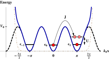
Figure 1: (Color online) Visualization of the “hopping”-parameter $J$, the onsite energies $\epsilon_{i}\;(i=0,\pm 1)$ and the interaction strength $U$. The potentials $V_{22}(\vec{r}\,)$ (blue solid), $V_{\rm OL}(\vec{r}\,)$ (black dashed) and $V_{\rm conf}(\vec{r}\,)$ (brown dash-dotted) are depicted for $y=z=0$.

II.2 Bose-Hubbard model

The periodicity of the OL potential gives rise to band gaps in the dispersion relation $E(\vec{k}\,)$. In contrast to a real solid, both the dispersion relation and the Bloch solutions of the Hamiltonian $\hat{H}_{\rm OL}=\frac{\hat{p}^{2}}{2m}+\hat{V}_{\rm OL}$ are known analytically. The extents of the first four Bloch bands of a one-dimensional OL are depicted as a function of the lattice depth $V_{0}$ in Fig. 2. For increasing lattice depths the band widths shrink and the gaps between the bands increase. Especially, the gap between the first and the second band prevents ultracold Bosons from occupying others than the lowest Bloch band. The energy of states in this band can be roughly approximated by the ground state energy $\hbar\omega/2$ of the harmonic approximation. However, even for $V_{0}\gg\hbar\omega$ there is a constant energy offset of $E_{r}/4$ between the harmonic approximation and the exact ground state energy. This offset is a result of the anharmonicity of the lattice sites. It can be explained by a perturbation of the harmonic ground-state energy by the next-to-leading order expansion ($\sim x^{4}$) of the OL potential Slater (1952).

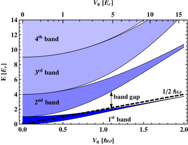
Figure 2: (Color online) Extents of the lowest four energy bands of the one-dimensional optical lattice as a function of the lattice depth $V_{0}$. The energy of the first band can be approximated by the harmonic ground-state energy $\frac{1}{2}\hbar\omega$ (dashed line). A better approximation includes a constant energy offset of $E_{r}/4$ (see the text).

The BHM makes use of the basis of Wannier functions, constructed with the aid of the known Bloch solutions of the lowest band to approximate the triple-well Hamiltonian $\hat{H}_{\rm trip}$. In the case of an infinite OL with no interaction this orthogonal basis spans completely the Hilbert space of the first Bloch band. In contrast to the Bloch solutions, each Wannier function $w_{j}(\vec{r}\,)$ is localized at one lattice site $j$. Wannier functions can be constructed in many different ways depending on the choice of phases of the Bloch solutions. In accordance to the widely used convention of the BHM we consider the form specified by Kohn in Kohn (1959) which leads to maximally localized, real Wannier functions.

To describe systems with a finite number of wells, the amount of Bloch solutions is usually restricted to those which fulfill periodic boundary conditions. For the triple-well potential used in this work, the boundaries may be set to $k_{0}x_{B}=\frac{3\pi}{2}$ or, in order to probe the outer potential walls, to $k_{0}x_{B}=2\pi$. These conditions change slightly the shape of the Wannier functions.

We adapt the basis to the triple-well potential by using in $y$- and $z$-direction the appropriate harmonic ground-state solution $h_{0}$ instead of the Wannier function for a one-well lattice. The adapted Wannier functions read

$$w_{j}(\vec{r}\,)=w_{j}^{\rm 1D}(x)h_{0}(y)h_{0}(z).$$ (4)

A detailed description of Wannier functions can be found in Refs. Kohn (1959); Jaksch and Zoller (2005).

Let $\hat{b}_{j}^{\dagger}$ ($\hat{b}_{j}$) be the bosonic operator of creation (annihilation) of a particle with the Wannier function $w_{j}(\vec{r}\,)=\left<\vec{r}\,|w_{j}\right>$, then $\hat{H}_{\rm trip}$ (Eq. 3) is written in the Wannier basis as

$$\begin{split}\hat{H}_{\rm Wan}=&\sum_{i,j}\left<w_{i}\right|\frac{\hat{p}^{2}}{2m}+\hat{V}_{\rm OL}+\hat{V}_{\rm conf}\left|w_{j}\right>\hat{b}^{\dagger}_{i}\hat{b}_{j}+\\ \frac{1}{2}&\sum_{k,l,m,n}\left<w_{k}\right|\left<w_{l}\right|\hat{V}_{\rm int}\left|w_{m}\right>\left|w_{n}\right>\hat{b}^{\dagger}_{k}\hat{b}_{l}^{\dagger}\hat{b}_{m}\hat{b}_{n},\end{split}$$ (5)

with all indices running over $-1,0,+1$.

This is already the first approximation of the BHM as the Wannier basis is only complete for the first Bloch band if $\hat{V}_{\rm int}=0$ and $\hat{V}_{\rm conf}=0$. The BHM further simplifies $\hat{H}_{\rm Wan}$ by making the following assumptions: (i) The overlap between Wannier functions on different lattice sites is small. This reduces the $i,j$-summation to diagonal elements $i=j$ and neighboring lattice sites $\left<i,j\right>$. (ii) The confinement potential $\hat{V}_{\rm conf}$ varies slowly and does not couple Wannier functions at different lattice sites, i. e. $\left<w_{i}\right|\hat{V}_{\rm conf}\left|w_{j}\right>=0$ for $i\neq j$. (iii) The interaction is short-ranged and only takes place between particles in the same well.

Applying these assumptions, the final BH Hamiltonian takes the form

$$\hat{H}_{\rm BH}=-J\sum_{<i,j>}\hat{b}^{\dagger}_{i}\hat{b}_{j}+\frac{U}{2}\sum_{i}\hat{b}^{\dagger}_{i}\hat{b}_{i}^{\dagger}\hat{b}_{i}\hat{b}_{i}+\sum_{i}\epsilon_{i}\hat{b}^{\dagger}_{i}\hat{b}_{i},$$ (6)

with the hopping parameter $J=-\left<w_{0}\right|\frac{\hat{p}^{2}}{2m}+\hat{V}_{\rm OL}\left|w_{1}\right>$, the onsite energies $\epsilon_{i}=\left<w_{i}\right|\frac{\hat{p}^{2}}{2m}+\hat{V}_{\rm OL}+\hat{V}_{\rm conf}\left|w_{i}\right>\,(i=0,\pm 1)$ and the interaction parameter $U=\left<w_{0}\right|\left<w_{0}\right|\hat{V}_{\rm int}\left|w_{0}\right>\left|w_{0}\right>$. Even though the BH Hamiltonian has a simple form, there does not exist a general solution for large lattices with many particles. However, for two particles in a triple well the BH Hamiltonian is easily diagonalizable.

The integrations occuring in the definition of the BH parameters are performed consistently within the periodic boundary conditions of $x$. The Bloch functions which are used to construct the Wannier functions are also normalized to one within the boundaries. Since the trapping potential is symmetric, $\epsilon_{-1}=\epsilon_{+1}$ holds. For a visualization of the BH parameters see Fig. 1.

A further important approximation, which is very common in the physics of ultracold atomic gases, is the replacement of the full BO interaction potential by a point-like pseudopotential Busch et al. (1998)

$$V_{\rm ps}(\vec{r}\,)=\frac{4\pi\hbar^{2}a_{\rm sc}}{m}\delta^{(3)}(\vec{r}\,)\frac{\partial}{\partial r}r$$ (7)

that depends only on the s-wave scattering length $a_{\rm sc}$. This simplifies the integration for the interaction parameter drastically to

$$U=\frac{4\pi\hbar^{2}a_{\rm sc}}{m}\int{\rm d}^{3}\vec{r}\,\left|w_{0}(\vec{r}\,)\right|^{4}.$$ (8)

The formulations of $J,U,\epsilon_{0},$ and $\epsilon_{\pm 1}$ described above are in the following denoted as the “BH representation” of the parameters and will be indicated with the superscript “BH”.

It should be noted that not only the Wannier basis leads to the form of the BH Hamiltonian (Eq. 6). Any other nearly orthogonal basis of functions localized in one of the wells leads to the same form, with only different values of the parameters. The usual basis of the BH Hamiltonian of two particles in a triple well is the occupation-number basis $\{\left|002\right>,\left|011\right>,\left|101\right>,\left|020\right>,\left|110\right>,\left|200\right>\}$ which specifies the amount of particles in the left, middle and right well. In this respect it is even possible to think of a two-particle instead of a one-particle basis to arrive at the BHM. As a result, the BH Hamiltonian is principally able to describe strongly interacting particles without the need to expand the full Hamiltonian (1) in a large basis of one-particle Wannier functions of several Bloch bands. It is hence natural to imagine that there is a basis for the BHM which is far better adapted to an OL with interacting particles in the presence of a confining potential $\hat{V}_{\rm conf}$ than the Wannier basis. Although this optimal basis is unknown, it allows us to vary the BH parameters in order to adapt the model to the full numerical solution as is described below.

III Method

III.1 Numerical calculation in the triple well

To perform the full numerical calculation of the eigenenergies and eigenfunctions of Hamiltonian $\hat{H}_{\rm trip}$ the approach described in Grishkevich and Saenz is adopted. Briefly, in this method the lattice potential is expanded into a Taylor series and the resulting Hamiltonian is written as a sum of center-of-mass (COM) Hamiltonian $\hat{H}_{\rm COM}$, relative-motion (REL) Hamiltonian $\hat{H}_{\rm REL}$ and coupling terms $\hat{W}$. The eigenfunctions and eigenvalues of $\hat{H}_{\rm COM}$ and $\hat{H}_{\rm REL}$ are calculated separately in a basis of spherical harmonics $Y_{l}^{m}(\theta,\phi)$ times B splines $B_{\alpha}(r)$. The position of knots of the B splines in REL can be adjusted to adequately describe both the long range behavior in the trap ($\sim 10^{4}a_{0}$) and the short range behavior due to the molecular (interatomic) interaction ($\sim 65a_{0}$). The full solution including the coupling $\hat{W}$ is calculated from the eigenfunctions of $\hat{H}_{\rm COM}$ and $\hat{H}_{\rm REL}$ by the configuration-interaction (CI) method which is also known as exact diagonalization. The code is adapted to the symmetry group $D_{2h}$ of a cubic three-dimensional OL, which simplifies the calculation and allows to reduce the REL basis to functions which are symmetric under inversion and describe therefore Bosonic particles.

In Ref. Grishkevich and Saenz , a Taylor expansion up to the sixth order of the OL is used to examine the two-particle interaction in a single well. The ground state was described by a basis which consisted of angular components up to $l=3$. The triple well considered in the present work demands much higher angular components owing to its high degree of anisotropy. We need an expansion up to $l=32$ and about 70 B splines in COM and an expansion up to $l=30$ and 130 B splines in REL to obtain converged solutions for lattice depths up to $V_{0}=12E_{r}$. Altogether, about $16\ 000$ basis functions are used to describe the REL eigensolutions and $11\ 000$ to describe the COM eigensolutions. From these solutions about $10\ 000$ configurations form the basis of the CI calculations.

To tune the s-wave scattering length $a_{\rm sc}$ to values in the range $a_{\rm sc}\in(-\infty,+\infty)$ the inner wall of the BO potential is slightly shifted as suggested in Ref. Grishkevich and Saenz . This procedure can move the least bound state close to the dissociation threshold or leads to the creation of a new bound state. Simultaneously the scattering length grows to $+\infty$ or $-\infty$, respectively, which offers a knob to vary $a_{\rm sc}$ in a controlled way.

III.2 Numerical Determination of the optimal BH parameters

The numerical determination of the optimal BH parameter set is done by fitting the parameters $\mathcal{P}=(J,\epsilon_{0},\epsilon_{\pm 1},U)$ such that an optimal agreement between the eigenenergies of the BH Hamiltonian and the full numerical solution is achieved.

In more detail, let

$$\hat{H}_{\rm trip}\left|\Psi_{i}\right>=E_{i}\left|\Psi_{i}\right>$$ (9)

be the stationary solution of the triple-well Hamiltonian and

$$\hat{H}_{\rm BH}^{\mathcal{P}}\left|\Phi_{j}^{\mathcal{P}}\right>=\mathcal{E}_{j}^{\mathcal{P}}\left|\Phi_{j}^{\mathcal{P}}\right>$$ (10)

be the stationary solution of the BH Hamiltonian $\hat{H}_{\rm BH}^{\mathcal{P}}\equiv\hat{H}_{\rm BH}$ with parameter set $\mathcal{P}$. Due to the restriction to one basis function per particle and lattice site, the second eigenvalue equation has only six solutions with energies $\mathcal{E}_{1}^{\mathcal{P}},\dots,\mathcal{E}_{6}^{\mathcal{P}}$.

With the aid of the eigenenergies, we obtain the optimal set of BH parameters $\mathcal{P}^{\rm opt}$ by minimizing the measure

$$f(\mathcal{P})=\sum_{i=1}^{6}\left(\frac{E_{i}-\mathcal{E}_{i}^{\mathcal{P}}}{E_{i}}\right)^{2}.$$ (11)

However, a fit of all four parameters at once is problematic. Since only six eigenenergies exist, a local minimum of $f(\mathcal{P})$ may be found that leads to a non-optimal parameter set $\mathcal{P}$. On the other hand, it is inherent to the BHM, that all effects due to interaction are contained in the interaction parameter $U$ leaving the other parameters unaffected. Therefore, we determine the optimal parameter set in a two-step process: (i) The parameters $J,\epsilon_{0},\epsilon_{\pm 1}$ are fitted to match the energies of a numerical calculation without interaction. (ii) The parameter $U$ is fitted to match the energies of a numerical calculation with interaction, keeping the other BH parameters fixed to the values of the previous fit.

III.3 Estimation of the interaction parameter $U$

As already mentioned, the Wannier functions do not reflect effects of interaction. Being a one-particle basis, the Wannier basis is only complete for non-interacting particles. Thus, one cannot assume that in strong interacting regimes the BH representation of the interaction parameter given in Eq. (8) is applicable and one should estimate the energy offset caused by interaction differently.

Fortunately, an analytical solution is known for a system of two identical particles in an isotropic or anisotropic harmonic trap interacting only via the pseudopotential of Eq. (7) Busch et al. (1998); Idziaszek and Calarco (2005). While for no interaction ($a_{\rm sc}=0$) the eigenenergies in the isotropic case are given as $E_{n,l}=\hbar\omega(\frac{3}{2}+2n+l)$, a non-vanishing scattering length leads to a shift of all eigenenergies with $l=0$. The dependence of the energies $E_{n,l=0}$ on the scattering length is shown in Fig. 3 and is given by the solution of the implicit equation

$$\frac{a_{\rm sc}}{a_{\rm ho}}=\frac{1}{2}\tan\left(\frac{\pi\epsilon}{2}+\frac{\pi}{4}\right)\frac{\Gamma\left(\frac{\epsilon}{2}+\frac{1}{4}\right)}{\Gamma\left(\frac{\epsilon}{2}+\frac{3}{4}\right)},$$ (12)

where $\epsilon=E/\hbar\omega$ and $\Gamma$ denotes the Gamma function Bolda et al. (2002). Additionally, for positive scattering lengths one bound eigensolution appears (lowest branch). For ultracold atoms only the first two states with energies lower than $E_{0,1}=\frac{5}{2}\hbar\omega$ should be occupied. This corresponds to the reduction to the first Bloch band in the OL.

The known energy spectrum offers the possibility to estimate the energy offset due to interaction as a function of the scattering length. As shown in Fig. 3, for positive scattering lengths one has the choice between two branches; one with a negative offset $\Delta E_{\rm harm}^{0}$ to the lower branch and one with a positive offset $\Delta E_{\rm harm}^{1}$ to the upper branch. For negative $a_{\rm sc}$ only the latter branch exists and $\Delta E_{\rm harm}^{1}$ is negative.

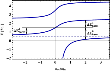
Figure 3: (Color online) Analytical energy spectrum of relative-motion $l=0$ states of two particles interacting by the potential $\hat{V}_{\rm ps}$ (Eq. 7) in a harmonic trap as a function of the scattering length. The spectrum defines the energy offsets $\Delta E_{\rm harm}^{0}$ and $\Delta E_{\rm harm}^{1}$ relative to the ground-state energy in the absence of interaction, $\frac{3}{2}\hbar\omega$.

Since the interaction of the BHM has purely onsite character, one can expect that these energy offsets provide a good first approximation $U^{\rm harm}=\Delta E_{\rm harm}^{0,1}$ of the interaction parameter for strong interaction. Depending on which offset is chosen lower or higher parts of the energy spectrum may be modeled. The confinement in the harmonic trap is, however, stronger than in a sinusoidal OL. Thus, one can expect that the harmonic approximation tends to overestimate the strength of the onsite interaction in the OL.

Despite the weakness of the Wannier basis for strong interaction it can offer crucial information on anharmonic effects. Its completeness for $\hat{V}_{\rm int}=0$ and $\hat{V}_{\rm conf}=0$ allows an almost exact prediction of the behavior of $U$ for $a_{\rm sc}\rightarrow 0$. (To first order, $\hat{V}_{\rm conf}$ has no influence on $U$.) This observation can be used to define a correction factor $\mathcal{A}$ to the harmonic approximation which accounts for anharmonic effects. The factor is defined by demanding that $\mathcal{A}\cdot\Delta E_{\rm harm}^{1}$ has the same linear behavior as $U^{\rm BH}$ for $a_{\rm sc}\rightarrow 0$, i. e.

$$\mathcal{A}\cdot\left(\frac{\rm d}{da_{\rm sc}}\Delta E_{\rm harm}^{1}\right)_{a_{\rm sc}\rightarrow 0}\stackrel{{\scriptstyle!}}{{=}}\frac{{\rm d}U^{\rm BH}}{da_{\rm sc}}$$

$$\Rightarrow\mathcal{A}=\frac{\sqrt{\pi}a_{\rm ho}}{2\hbar\omega}\cdot\frac{4\pi\hbar^{2}}{m}\int{\rm d}^{3}\vec{r}\,\left|w_{0}(\vec{r}\,)\right|^{4}.$$ (13)

Remarkably, the factor $\mathcal{A}$, which is shown in Fig. 4 for different lattice depths $V_{0}$, approaches even for very deep lattices only slowly unity. Thus it is needed to correct the harmonic approximation even for very deep lattices. For shallow lattices the factor rises above one and goes for $V_{0}\rightarrow 0$ to $+\infty$. This is due to the fact that periodic boundary conditions are implied. Thus, the normalization of the Wannier functions within the boundaries prevents the integral in the BH representation of $U$ to vanish for $V_{0}\rightarrow 0$ while $a_{\rm ho}/\hbar\omega$ goes to infinity.

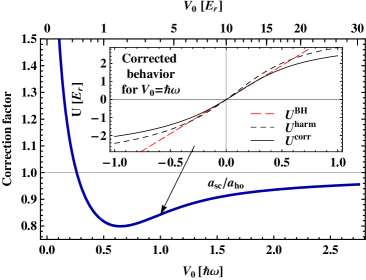
Figure 4: (Color online) The correction factor $\mathcal{A}$ as a function of the lattice depth $V_{0}$. Inset: Comparison of $U^{\rm BH}$, $U^{\rm harm}$, and $U^{\rm corr}$ for $V_{0}=\hbar\omega$ as a function of the scattering length. In accordance with the definition of $\mathcal{A}$ the behavior of $U^{\rm BH}$ and $U^{\rm corr}$ matches for small $a_{\rm sc}$.

The validity regime of the corrected harmonic approximation $U^{\rm corr}\equiv\mathcal{A}U^{\rm harm}$ depends on the applicability of the pseudopotential approximation with an energy-independent scattering length used in $U^{\rm harm}$ and the validity range of $\mathcal{A}$. The latter can be roughly predicted by considering that the correction factor accounts for the different confinement in the harmonic trap and the real OL for a certain ground state energy $E$ of noninteracting particles. In order for $\mathcal{A}$ to be valid for $a_{\rm sc}\neq 0$, the deviation of the energy ($\approx U$) should be small compared to the depth of the lattice $V_{0}$, which simply means

$$|U|\approx|U^{\rm corr}|\ll V_{0}.$$ (14)

This is to some extent counter-intuitive as for a fixed scattering length $a_{\rm sc}$ an increase of $V_{0}$ is accompanied by an increase of $|a_{\rm sc}/a_{\rm ho}|$. This leads to a breakdown of the BH representation and to errors caused by the use of an energy-independent scattering length in $U^{\rm harm}$. Since at the same time the error of the correction factor $\mathcal{A}$ shrinks it is important to quantify and compare the different errors in order to understand when $U^{\rm corr}$ is applicable.

III.4 Sextic approximation

An alternative way to look at effects of anharmonicity on the interaction is to consider an optical lattice not expanded to second or twenty-second but to the sixth order in $x$-direction. This sextic trap consists of one well, but includes anharmonic effects and coupling between relative and center-of-mass motion Grishkevich and Saenz . The energy difference of two atoms in a sextic well with and without interaction defines the interaction parameter $U^{\rm sext}$.

III.5 Energy-dependent scattering length

The scattering length used in the pseudopotential (Eq. 7) is defined by the s wave of a trap-free scattering process in the limit of zero collision energy. The solution in the trap has, however, a different asymptotic behavior and a finite ground-state energy. Much work has been devoted to the question when a pseudopotential can be used in a trap and which scattering length should be chosen for energies greater than zero Gao (1998); Tiesinga et al. (2000); Block and Holthaus (2002); Bolda et al. (2002). It has been shown that the use of an energy-dependent effective scattering length can largely extend the range of validity of the pseudopotential approximation towards strong confinement and strong interaction in harmonic traps Blume and Greene (2002); Bolda et al. (2002); Grishkevich and Saenz .

To quantify the impact of the energy dependence independently of anharmonic effects we consider two ⁷Li atoms in a harmonic trap and determine numerically the ground-state energy. Plugging this energy into the right-hand side of Eq. (12) defines the “optimal” scattering length $a_{\rm opt}$ for the description of the interaction by the pseudopotential. In its range of validity the effective scattering length is equal to the optimal scattering length.

The numerical calculation with the full BO interaction in an OL makes it possible to compare the effect of an energy-dependent scattering length to effects caused by the anharmonicity of the OL and the incompleteness of the Wannier basis.

IV Results

This section is devoted to a comparison of the analytical approaches to describe interacting particles in a triple well with the full numerical results which determine the optimal BH parameters. First, the interaction-independent parameters $J,\epsilon_{0},\epsilon_{\rm\pm 1}$ are considered for a varying lattice depth $V_{0}$. Then the discussion is extended to interacting particles for both different lattice depths and different scattering lengths.

Here a short overview of the abbreviations used in the following.

BH	Parameters in BH representation and eigenenergies of the BHM with these parameters.
harm	The same as “BH” but with $U^{\rm harm}$ determined in the harmonic trap.
corr	The same as “BH” but with the corrected $U^{\rm corr}=\mathcal{A}\cdot U^{\rm harm}$.
opt	The optimal BH parameters and eigenenergies of the BHM with these parameters. This abbreviation is also used for the optimal scattering length.
sext	Interaction parameter $U^{\rm sext}$ obtained from the sextic approximation of the OL.
num	The eigenenergies of the full numerical CI calculation.

IV.1 Onsite energies

The optimal onsite energies for the middle well and the outer wells are shown in Fig. 5. On the first glance, they seem to be very well matched by the corresponding BH representations. However, by subtracting the value of the onsite energy for no confinement $\left<w_{0}\right|\frac{\hat{p}^{2}}{2m}+\hat{V}_{\rm OL}\left|w_{0}\right>$ in the inset of Fig. 5 the impact of $\hat{V}_{\rm conf}$ on the BH representation and the optimal values of the onsite energies can be examined. Generally, the shallower the lattices the more the optimal onsite energies of both wells are lifted by the confinement. Only for $V_{0}>\hbar\omega$ this trend is reflected by the BH representation, while for shallower lattices boundary conditions at $k_{0}x_{B}=3\pi/2$ underestimate the impact of the confinement. On the other hand, for $k_{0}x_{B}=2\pi$ (not shown in the graph) the boundary reaches deep inside the walls of the confinement and the BH representation extremely overestimates $\epsilon_{\pm 1}$ for $V_{0}<1.7\,\hbar\omega$ and even $\epsilon_{0}$ for $V_{0}<0.8\,\hbar\omega$.

A reason for the inaccuracy of the BH representation of $\epsilon_{0}$ and $\epsilon_{\pm 1}$ is that only for a slowly varying confining potential $V_{\rm conf}(\vec{r}\,)$ the Wannier functions form a good basis. As $V_{\rm conf}(\vec{r}\,)$ varies strongly for $|k_{0}x|>\frac{3\pi}{2}$ the lattice must be considerably deep so that the particles do not “see” the form of the boundary and the distance $x_{B}$ of the boundary conditions must be sufficiently small not to reach inside the region of the strong increase of the confining potential (see Fig. 1). For boundary conditions at $k_{0}x_{B}=3\pi/2$ and lattice depths $V_{0}>1.5\,\hbar\omega$ both the values of the onsite energies and their two orders of magnitude smaller differences are well described by the BH representation. It can be assumed that for larger lattices with smooth harmonic trapping potentials, the BHM converges faster.

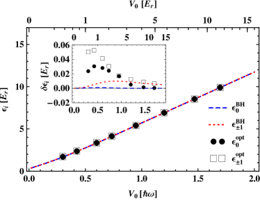
Figure 5: (Color online) Onsite energies as a function of the lattice depth $V_{0}$: the optimal values together with the BH representation for the middle well ($\epsilon_{0}$) and the outer wells ($\epsilon_{\pm 1}$) for $k_{0}x_{B}=3\pi/2$.
Inset: In order to examine the impact of the confining potential $\hat{V}_{\rm conf}$ the value of $\delta\epsilon_{i}=\epsilon_{i}-\left<w_{0}\right|\frac{\hat{p}^{2}}{2m}+\hat{V}_{\rm OL}\left|w_{0}\right>$ is depicted, where the value of the onsite energy for no confinement is subtracted. Clearly, for $V_{0}>1.5\,\hbar\omega$ both results are converged.

IV.2 Hopping parameter

As in the case of the onsite energies, the confining potential can cause also problems for the prediction of the hopping parameter. Fig. 6 (a) shows the optimal hopping parameter and its BH representation for different boundary conditions $k_{0}x_{B}=3\pi/2,2\pi$ and $\infty$. One can see that the choice of the boundary conditions influences considerably the BH representation for shallow lattices. It seems that in this special case boundaries at $2\pi$ or infinity produce the best prediction. However, similarly to the case of the onsite energies all BH representations predict the correct hopping parameter for $V_{0}>1.5\,\hbar\omega$. The reason is analogous. The BHM assumes that $\hat{V}_{\rm conf}$ is approximately constant within one well. Therefore, due to the orthogonality of the Wannier functions, $\left<w_{0}\right|\hat{V}_{\rm conf}\left|w_{1}\right>=0$ holds. This is essential for the definition of the hopping parameter, where the influence of the confinement potential is neglected. However, as described in the last paragraph, for shallow lattices the form of the boundary becomes important and strongly varying parts of the potential are probed. One can expect an error of the BH representation for $J$ of the size $\Delta J=\left<w_{0}\right|\hat{V}_{\rm conf}\left|w_{1}\right>$ which is negligible only for sufficiently deep lattices.

Energy spectrum for no interaction

Since the BH representation of both the hopping and the onsite-energy parameter is converged for $V_{0}>1.5\,\hbar\omega$, the BHM predicts the correct eigenenergies in this regime. The mean deviation from the numerical energies for $V_{0}=1.7\,\hbar\omega$ is $0.25E_{r}$ or $0.01\%$ respectively. Fig. 6 (b) shows the spectrum of the full numerical calculation. In order to compensate for an increase of the energies of the order of $2\epsilon_{0}$ and the shrinking width of the first Bloch band of the order of $4J$ as $V_{0}$ is increased, rescaled energies $\eta_{i}$ with

$$\eta_{i}(V_{0})=\frac{E_{i}-2\epsilon_{0}^{\rm BH}}{4J^{\rm BH}}$$ (15)

are shown. For $V_{0}>1.5\,\hbar\omega$ the spectrum of the BH Hamiltonian in the BH representation is in very good agreement with the spectrum obtained from a full numerical calculation. With the optimal parameter set the BHM is able to predict the numerical eigenenergies already for $V_{0}>\hbar\omega$ with high accuracy (mean relative error in energies $\approx 0.001\%$). For shallower lattices numerical and optimal eigenenergies do not match, which means that the BHM is principally unable to reproduce the eigenenergies of the triple well for $V_{0}<\hbar\omega$. Two differences are most obvious: (i) Both the BHM in the BH representation and with the optimal BH parameters underestimate significantly the value of the ground-state energy while especially the BH representation tends to overestimate all other eigenenergies in the limit of vanishing lattice depth. (ii) For $U=0$ the BHM predicts an energy difference of $\epsilon_{1}-\epsilon_{0}$ between the third and fourth energy level. In the BH representation this difference goes to zero for $V_{0}\rightarrow 0$ (see Fig. 5) and the levels become degenerate. Although this degeneracy is lifted by using the optimal parameter set, the energy difference is still largely underestimated.

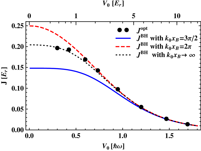
(a) (b)

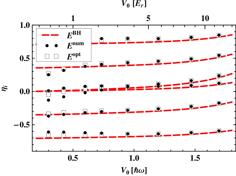
Figure 6: (Color online) (a) Hopping parameter $J$ as a function of the lattice depth $V_{0}$: the optimal value together with the BH representation for $k_{0}x_{B}=\frac{3}{2}\pi,2\pi,\infty$. (b) The six eigenenergies in the rescaled form (see Eq. (15)) for $a_{\rm sc}=0$ and $U=0$ as a function of the lattice depth $V_{0}$. The BH energies are obtained for onsite energies with boundaries at $k_{0}x_{B}=3\pi/2$ and a hopping parameter with boundaries at $k_{0}x_{B}=2\pi$.

These disagreements can be caused by the dominance of the confinement potential over the OL potential for small lattice depths. Also hopping to non-neighboring wells can become important as shown in Sec. IV.4. As already mentioned, one can assume that the BHM converges better for larger lattices with a shallow harmonic external confinement. On the other hand, the convergence behavior for, e. g., double wells as they appear in superlattices should be similar or even worse compared to the case of the triple well.

IV.3 Interaction parameter

The interaction parameter $U$ depends on both the scattering length $a_{\rm sc}$ and the lattice depth $V_{0}$ that determines how strong two particles are confined in one well. First, the dependence on the lattice depth for the case of a relatively small and a relatively large negative scattering length will be discussed.

Fig. 7 (a) shows a plot of the optimal interaction parameter $U^{\rm opt}$ together with several predictions of the interaction energy by $U^{\rm BH},U^{\rm harm}$ and $U^{\rm corr}$. The scattering length is fixed to about $-180a_{0}$. For this value, the ratio $\left|a_{\rm sc}/a_{\rm ho}\right|$ which increases with the lattice depth $V_{0}$ reaches up to only $0.08$ in this graph.

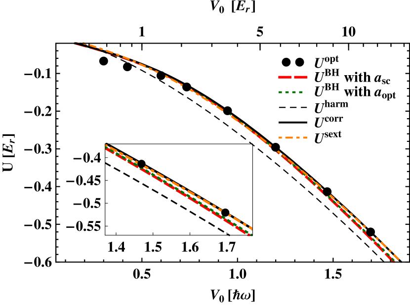
(a) (b)

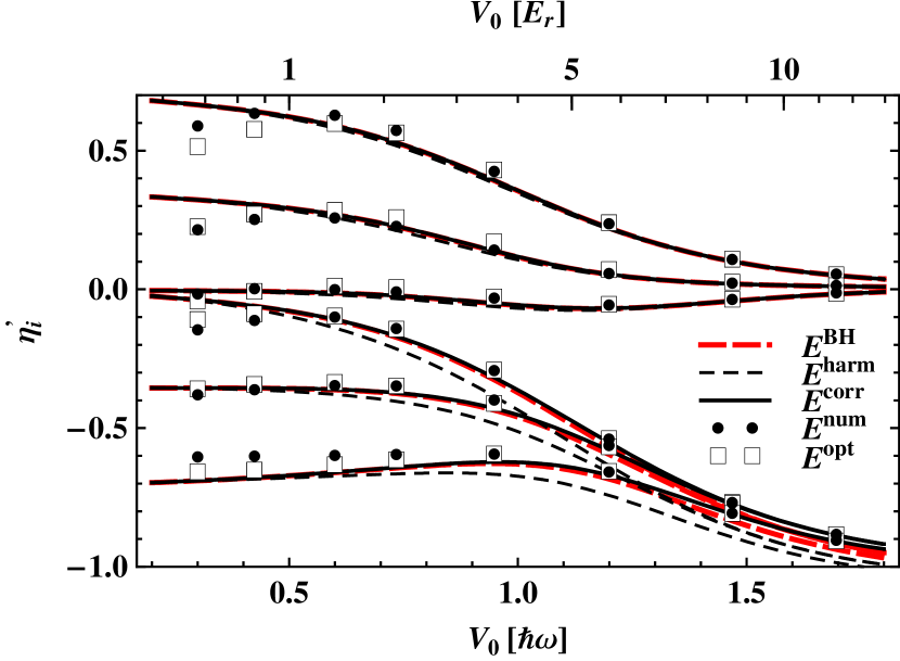
Figure 7: (Color online) (a) The Interaction parameter as a function of the lattice depth $V_{0}$ in the weak interacting regime with $a_{\rm sc}\approx-180a_{0}$. This results in $0.02\leq\left|a_{\rm sc}/a_{\rm ho}\right|\leq 0.08$ in this graph. (b) The six eigenenergies in the rescaled form (see Eq. (16)) as a function of the lattice depth $V_{0}$.

Within the BHM the interaction parameter $U^{\rm BH}$ is independent of the confining potential $\hat{V}_{\rm conf}$. Accordingly, the main source of error is not that the Wannier functions are not adapted to the confining potential, but that they do not reflect effects of interaction. Thus, for weak interaction the BH representation predicts $U^{\rm opt}$ quite well already for shallow lattices with $V_{0}\approx\hbar\omega$. However, an increasing value of $V_{0}$ amplifies the confinement and thus the ratio $\left|a_{\rm sc}/a_{\rm ho}\right|$. Remarkably, this causes a small error of $U^{\rm BH}$ which is already visible for $\left|a_{\rm sc}/a_{\rm ho}\right|<0.08$ and reduces the validity regime of $U^{\rm BH}$ to scattering lengths which are at least one order of magnitude smaller than the trap length $a_{\rm ho}$.

For weak interaction the energy-offset in the harmonic well $U^{\rm harm}$ can predict $U^{\rm opt}$ only poorly compared to $U^{\rm BH}$. On the other hand, the corrected analytical approach $U^{\rm corr}$ introduced in Sec. III.3 is in excellent agreement with the optimal interaction parameter for $V_{0}>\hbar\omega$. This is also reflected by the energy spectrum shown in Fig. 7 (b).

In Fig. 7 (b) the upper three states describe particles in different wells with energies almost independent of the interaction. The first three states, on the other hand, describe attractively interacting particles in the same well. Within the BHM their energies are shifted in the order of $U$. Thus, the rescaling of the energies (Eq. 15) is changed to

$$\eta_{i}^{\prime}(V_{0})=\frac{E_{i}-2\epsilon_{0}^{\rm BH}}{4J^{\rm BH}+|U^{\rm corr}|}.$$ (16)

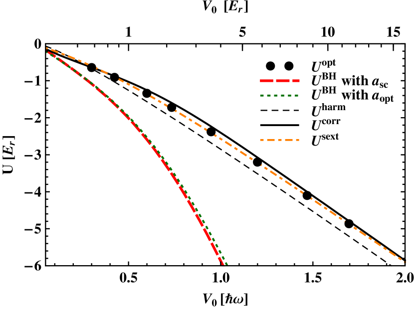
(a) (b)

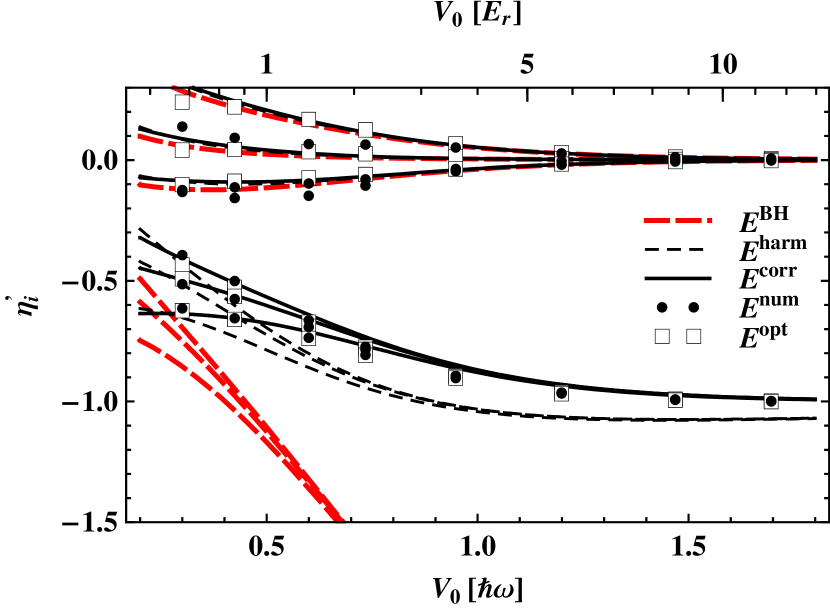
Figure 8: (Color online) (a) The Interaction parameter as a function of the lattice depth $V_{0}$ in the strong interacting regime with $a_{\rm sc}\approx-4600a_{0}$. This results in $0.5\leq\left|a_{\rm sc}/a_{\rm ho}\right|\leq 2.2$ in this graph. (b) The six eigenenergies in the rescaled form (see Eq. (16)) as a function of the lattice depth $V_{0}$.

The energies of the lowest three states are well predicted by using $U^{\rm corr}$ for $V_{0}\geq 1.2\,\hbar\omega$ while both the BH representation and the harmonic approximation underestimate the energies more and more as the lattice depth and with this $|a_{\rm sc}/a_{\rm ho}|$ increases. For lattice depths smaller than $\hbar\omega$ the errors from the non-interacting case are inherited, e. g. the ground-state energy and the splitting between the third and the fourth level is underestimated by all models.

In Fig. 8 (a) the interaction parameter is plotted for a large negative scattering length of about $-4600a_{0}$ which means, that the absolute value of the scattering length is up to two times larger than the trap length $a_{\rm ho}$. As the magnitude of $a_{\rm sc}$ is of the order of $a_{\rm ho}$, the BH representation of $U$ differs drastically from the real interaction parameter. In this regime the linear dependence of $U^{\rm BH}$ on the scattering length leads to significantly wrong results (see the inset in Fig. 4). In this case, the energy offset $U^{\rm harm}$ provides a far better approximation, but it results in an almost constant underestimation of the optimal interaction strength as is evident from Fig. 8 (a). The corrected interaction parameter, on the other hand, gets closer to $U^{\rm opt}$ for deep lattices. The graph supports that Eq. (14) indeed reflects the validity regime of $\mathcal{A}$. As $U$ is approximately proportional to $V_{0}/\hbar\omega$ the ratio $V_{0}/|U^{\rm corr}|$ shrinks with an increasing lattice depth like $(\hbar\omega)^{-1}$ and $U^{\rm corr}$ approaches the optimal interaction parameter. The same is again reflected by the energy spectrum shown in Fig. 8 (b). Only $U^{\rm corr}$ is able to reproduce the numerical eigenenergies of the three lowest states in deep lattices, while $U^{\rm harm}$ generates an almost constant underestimation and $U^{\rm BH}$ a rapidly increasing underestimation of the numerical eigenenergies of these states.

IV.3.1 Sextic approximation

Figs. 7 (a) and 8 (a) show additionally the estimate of the interaction parameter using $U^{\rm sext}$, the interaction energy obtained in the sextic trap. It agrees precisely with the optimal parameter $U^{\rm opt}$ independently of the strength of interaction provided that $V_{0}>1.5\,\hbar\omega$. Also for shallower lattices, it is close to the optimal value. Thus, the examination of the interaction in a sextic trap Grishkevich and Saenz can already cover all anharmonic features of the onsite interaction for sufficiently deep lattices. This implies that one can treat the anharmonic form of a lattice site as a perturbation to the harmonic approximation to study interactions in OLs more realistically. For example, in Mentink and Kokkelmans (2009) this has been done by treating the difference between the OL potential and the harmonic approximation as a perturbing potential. The effects of the anharmonicity within a single site of an optical lattice have also been investigated non-perturbatively in Deuretzbacher et al. (2008).

IV.3.2 Energy-dependent scattering length

One could expect that the use of the optimal energy-dependent scattering length $a_{\rm opt}$ instead of $a_{\rm sc}$ can improve the value of $U^{\rm BH}$ (see Eq. (8)) significantly. This is, however, not the case, as can be clearly seen in Fig. 7 (a) and Fig. 8 (a). In the validity regime of the BH representation ($|a_{\rm sc}|\ll a_{\rm ho}$) the energy dependence of the scattering length seems not to be of importance. Also for strong interaction the offset between $U^{\rm BH}$ when used with $a_{\rm sc}$ or $a_{\rm opt}$ is small compared to the offset between any of the $U^{\rm BH}$ and $U^{\rm opt}$. In other words, the effect of the energy dependence of the scattering length in the OL is generally small compared to the error due to the use of the interaction-independent Wannier basis.

To quantify the effect of the energy-dependence, we use

$$\Delta U=\frac{U^{\rm harm}(a_{\rm sc})-U^{\rm harm}(a_{\rm opt})}{U^{\rm harm}(a_{\rm opt})},$$ (17)

the error of the interaction energy in the harmonic well, if $a_{\rm sc}$ is used instead of $a_{\rm opt}$. This estimates the error of neglecting the energy dependence of the scattering length independently of anharmonic effects. For a sufficiently large value of $|a_{\rm sc}/a_{\rm ho}|$ the deviation of $U^{\rm harm}$ from the linear behavior of $U^{\rm BH}$ (see inset of Fig. 4) starts to be significant. Therefore, the size of $a_{\rm sc}$ relative to $a_{\rm opt}$ does not directly show the impact of the energy dependence.

In Tab. 1 besides $\Delta U$ the errors of $U^{\rm BH}$, $U^{\rm harm}$ and $U^{\rm corr}$ compared to the optimal value are listed for various scattering lengths and lattice depths. For very deep lattices with $V_{0}>12E_{r}$ where a full numerical calculation in the triple well is too laborious we use the sextic approximation $U^{\rm sext}$ instead of the optimal interaction parameter, as it exactly reproduces $U^{\rm opt}$ for $V_{0}>10E_{r}$.

The value of $\Delta U$ in Tab. 1 shows to depend mainly on the ratio $a_{\rm sc}/a_{\rm ho}$. However, even for a large ratio it amounts up to only a few percent. Also the error of $U^{\rm BH}$ depends on that ratio, but grows much faster with $|a_{\rm sc}/a_{\rm ho}|$. This reflects again the complete breakdown of the BH representation for scattering lengths with a magnitude of the order of the trap length.

The error of $U^{\rm harm}$ decreases, though quite slowly, with growing lattice depth $V_{0}$. It comprises the error of an energy-independent scattering length ($\Delta U$) and of neglecting anharmonic effects. The latter effect can be estimated by subtracting the value of $\Delta U$ from the error of $U^{\rm harm}$. Only for the largest depth considered in Tab. 1 ($V_{0}=64.7E_{r}$) effects of $\Delta U$ are bigger than anharmonic effects. For a fixed lattice depth $V_{0}=11.5E_{r}$ and a decrease of the scattering length from $-0.08a_{\rm ho}$ to $-2.01a_{\rm ho}$ anharmonic effects seem to become less important. This can be explained by the stronger confinement in the wells due to the attractive interaction.

The error of $U^{\rm corr}$ results from the error of the correction factor $\mathcal{A}$ and from the error $\Delta U$. The error of $\mathcal{A}$ can again be estimated by subtracting $\Delta U$ from the error of $U^{\rm corr}$. This shows that the error of $\mathcal{A}$ depends, as expected, on the ratio $U^{\rm corr}/V_{0}$. In all considered cases it is found to be smaller than the error of $U^{\rm harm}$ caused by the anharmonicity and possesses the opposite sign of $\Delta U$. Therefore, the total error of $U^{\rm corr}$ is generally much smaller than the error of $U^{\rm BH}$ or $U^{\rm harm}$.

Table 1: The error $\Delta U$ of the use of an energy independent scattering length together with errors of $U^{\rm BH}$, $U^{\rm harm}$ and $U^{\rm corr}$ relative to $U^{\rm opt}$ for various lattice depths and scattering lengths.

$V_{0}/E_{r}$	11.5	11.5	25.2	64.7
$a_{\rm sc}/a_{\rm ho}$	-0.08	-2.01	-2.44	-3.09
$U^{\rm corr}/V_{0}$	-0.05	-0.42	-0.30	-0.20
$\Delta U$	-0.58%	-1.5%	-1.8%	-2.2%
Error of $U^{\rm BH}$	-3.18%	-190%	-243%	-320%
Error of $U^{\rm harm}$	-8.53%	-7.0%	-5.1%	-4.2%
Error of $U^{\rm corr}$	0.06%	1.5%	0.04%	-1.1%

IV.3.3 Interaction energy at a resonance of the scattering length

Until now the two cases of very small and very large interaction were discussed. To examine in more detail the regime of validity for $U^{\rm BH}$, $U^{\rm harm}$ and $U^{\rm corr}$ we consider in Fig. 9 the behavior of the interaction parameter at a resonance ($a_{\rm ho}/a_{\rm sc}\to 0$) for a lattice depth of $V_{0}=1.7\,\hbar\omega$. At this depth the BH representation of the other parameters ($J,\epsilon_{0}$ and $\epsilon_{\pm 1}$) is close to their optimal values.

Since at a resonance the energy regime of higher Bloch bands can be reached the notion of Bloch bands should be reconsidered in the presence of the new interaction parameters $U^{\rm harm}$ and $U^{\rm corr}$. For strong interaction one normally speaks of a coupling to higher Bloch bands, which means, that the true eigenfunctions can only be reproduced by an expansion into Wannier functions of several Bloch bands. The new interaction parameters are, however, not formulated as matrix elements in the Wannier basis. The resulting BH Hamiltonian is therefore intrinsicely a multi-band Hamiltonian. As shown in the last paragraphs the use of an optimal parameter set can reproduce the numerical energy spectrum very well. One can therefore describe multi-band physics surprisingly well within the simple BHM. As we will show now this has, however, limitations for repelling particles where the BH states become degenerate with excited “molecular” states and noninteracting ones in higher Bloch bands.

First of all, by varying the scattering length over the resonance ($a_{\rm ho}/a_{\rm sc}=0$) it becomes obvious, that the BH representation $U^{\rm BH}$ is not valid in the proximity of the resonance where it diverges to $\pm\infty$ (see Fig. 9 (a)). On the other hand, $U^{\rm corr}$ approximates well the optimal value $U^{\rm opt}$ for a large range of repelling (upper branch in Fig. 9 (a)) and attracting (lower branch in Fig. 9 (a)) interactions.

In Fig. 9 (b) the lower branch is shown on an enlarged scale around the resonance. It shows that $U^{\rm corr}$ is valid until $|a_{\rm sc}|\approx a_{\rm ho}$. For growing $|U|$ the correction factor $\mathcal{A}$ looses slowly its validity. Again, one can observe that the behavior of $U^{\rm opt}$ is exactly followed by the sextic approximation while the harmonic approximation generally overestimates the magnitude of $U^{\rm opt}$.

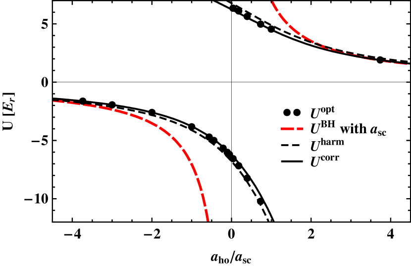
(a) (b)

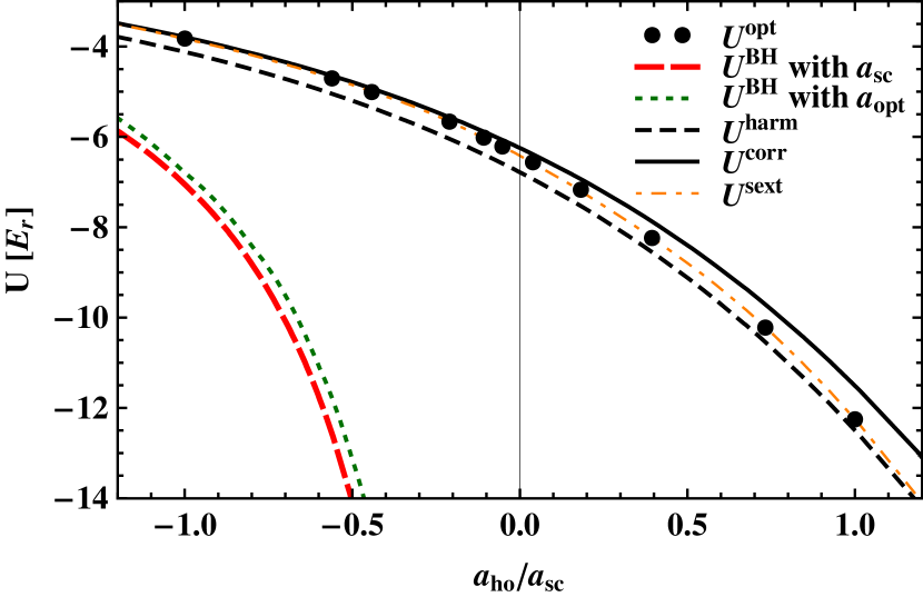
Figure 9: (Color online) The Interaction parameter for different scattering lengths at $\frac{V_{0}}{\hbar\omega}=1.7$. To observe the behavior at the resonance, the dependence on $\frac{a_{\rm ho}}{a_{\rm sc}}$ is shown.

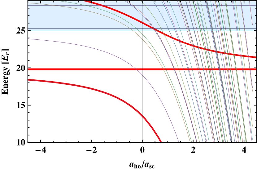
(a) (b)

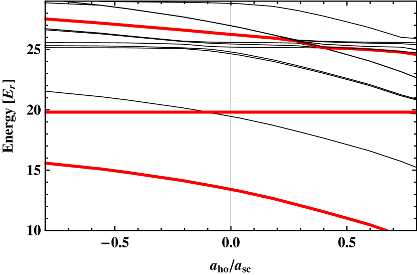
Figure 10: (Color online) Eigenenergies as a function of the scattering length at $\frac{V_{0}}{\hbar\omega}=1.7$. (a) Sketch of energy spectrum (see text for details). (b) Energy spectrum obtained from a full numerical calculation. The three thick (red) lines indicate energies which are closest to the energies predicted by the BHM.

On the upper branch in Fig. 9 near the resonance the energy of bound particles in higher Bloch bands can cross the BH states. To understand how this happens, we have sketched in Fig. 10 (a) a realistic estimate of a part of the energy spectrum. The spectrum has mainly three constituents: (i) The thick (red) lines represent the eigenvalues of the BHM of the first Bloch band (with $U=U^{\rm corr}$). The lower branch consists of three states with attracting particles ($U<0$) in the same well, and the upper branch of three states with repelling particles ($U>0$) in the same well. In the horizontal middle branch are all remaining energies with particles in different wells. These states are only weakly influenced by the interaction. (ii) The bunch of thin lines going from top to bottom represent “dimers” similar to the lowest BH states but in higher Bloch bands. Their energy consists of single-particle energies of Bloch states in different bands and the interaction energy $U^{\rm corr}<0$. (iii) The thin horizontal lines at the top represent the energies of non-interacting states where one particle is in the first Bloch band and one in the second Bloch band of at least one direction. The light (blue) filling indicates that the energy regime of higher Bloch bands is reached. Note, for any depth of the lattice two repulsively interacting particles will enter this energy regime at the resonance as it is always half way to the energy of two particles in the second Bloch band.

In Fig. 10 (b) we have plotted in the region of resonance the CI eigenenergies of the lowest totally symmetric states in the trap. As they are of the same symmetry, avoided crossings occur. These appear close to where the estimated energy spectrum (Fig. 10 (a)) shows (true) energy crossings. The avoided crossings are caused by a more or less strong coupling between states in different Bloch bands, which is not incorporated in the estimated spectrum. Particularly, the energy of states which can be identified with BH states of repulsively interacting particles is distorted due to avoided crossings. Thus, one cannot speak of pure repulsively interacting states in the first Bloch band any more. In contrast, the coupling between non-interacting BH states and the first exited “dimer” is very small and no energy distortion is visible at the resolution of Fig. 10 (b).

The complicated level structure indicates that the BHM, even if $U^{\rm corr}$ is used, has to be handled with care, if repulsively interacting and also non-interacting states at a resonance are to be described. In its corrected form it is, however, useful as a first approximation to find level crossings.

The rich structure of avoided crossings offers potentially a scheme to convert states of repulsively interacting, attractively interacting, and non-interacting nature into each other by performing sweeps of the scattering length. To estimate the dynamical behavior of the system the knowledge of the coupling strengths between states in different Bloch bands is crucial. Since these couplings are ignored within the BHM more sophisticated calculations such as the one presented in this work have to be performed to gain a deeper insight.

IV.4 Extended Bose-Hubbard model

Especially for shallow lattices both the interaction between particles in nearest-neighbor (NN) wells and hopping to next-to-nearest neighbors (NtNN) can become important Mazzarella et al. (2006); Boers et al. (2007); Trotzky et al. (2008). One can easily account for this by including the according matrix elements from $\hat{H}_{\rm Wan}$ of Eq. (5) into an extended Bose-Hubbard model (EBHM) with Hamiltonian

$$\begin{split}\hat{H}_{\rm EBH}=&\,\hat{H}_{\rm BH}+J_{2}(\hat{b}_{-1}^{\dagger}\hat{b}_{1}+\hat{b}_{1}^{\dagger}\hat{b}_{-1})\\ &+U_{1}\sum_{<i,k>}\left(\hat{b}^{\dagger}_{i}\hat{b}_{i}^{\dagger}\hat{b}_{i}\hat{b}_{k}+\hat{b}^{\dagger}_{i}\hat{b}_{k}^{\dagger}\hat{b}_{k}\hat{b}_{k}\right)\\ &+U_{2}\sum_{<i,k>}\left(\hat{b}^{\dagger}_{i}\hat{b}_{i}^{\dagger}\hat{b}_{k}\hat{b}_{k}+\hat{b}^{\dagger}_{i}\hat{b}_{k}^{\dagger}\hat{b}_{i}\hat{b}_{k}\right)\,.\end{split}$$ (18)

The NtNN hopping parameter $J_{2}=\left<w_{-1}\right|\frac{\hat{p}^{2}}{2m}+\hat{V}_{\rm OL}\left|w_{1}\right>$ decays much faster with the lattice depth than $J$. For $V_{0}=\hbar\omega$ it is one order smaller than $J$ and for $V_{0}=1.5\,\hbar\omega$ already two orders. Furthermore, the EBHM possesses in BH representation two new parameters $U_{1}=\frac{4\pi\hbar^{2}a_{\rm sc}}{m}\int d^{3}\vec{r}\,w_{0}(\vec{r}\,)^{3}w_{1}(\vec{r}\,)$, and $U_{2}=\frac{4\pi\hbar^{2}a_{\rm sc}}{m}\int d^{3}\vec{r}\,w_{0}(\vec{r}\,)^{2}w_{1}(\vec{r}\,)^{2}$, describing NN interaction. These parameters are generally at least one order of magnitude smaller than $U$. Unfortunately, the BH representation of $U_{1}$ and $U_{2}$ cannot be improved like for $U$ as there exists no analytical solution for two interacting particles in different wells. Therefore, only if the following conditions are met, the EBHM can be quantitatively better than the BHM: (i) The scattering length is small compared to the trap length (i. e. $|a_{\rm sc}|\ll a_{\rm ho}$), since otherwise $U_{1}$ and $U_{2}$ are predicted inaccurately. (ii) The lattice is deep enough that errors of the BH parameters are smaller than $U_{1}$, $U_{2}$ or $J_{2}$.

Fulfilling the first condition, the case of weak interaction ($a_{\rm sc}=-176\,a_{0}$) is discussed in the following. The second condition is not easy to meet in few-well systems, since especially the BH representation of the onsite-energies reflects the optimal parameters only for deep lattices (see the inset in Fig. 5), where $U_{1}$, $U_{2}$ and $J_{2}$ are already two orders of magnitude smaller than $U$ and $J$, respectively.

However, many observables do not depend on the absolute value of the eigenenergies, but on their differences. Energy differences determine for example the characteristic frequencies of a state in a coherent superposition of different eigenstates. These frequencies can be measured experimentally with high accuracy such that deviations of the simple BHM can be observed Trotzky et al. (2008).

The influence of the errors of the onsite energies can be reduced by considering differences of eigenenergies as the latter do not depend on the absolute value of the on-site energies but only on the offset $\Delta=\epsilon_{1}-\epsilon_{0}$. Although $\Delta$ is also predicted inaccurately in the BH representation for $V_{0}<1.2\,\hbar\omega$, it has often only a minor influence on the energy differences. This is especially the case for the energy difference $E_{5}-E_{2}$ for which a diagonalization of the BH Hamiltonian without interaction yields

$$E_{5}-E_{2}=\sqrt{J^{2}+\Delta^{2}}\,.$$ (19)

For the present potential with $V_{0}<1.2\,\hbar\omega$ the relation $J^{2}\gg\Delta^{2}$ holds. Since the errors of the parameters $J$ and $U$ are small for lattice depths down to $0.7\,\hbar\omega$, one can clearly identify effects of NN interaction and NtNN hopping as proper corrections of the BHM for this energy difference.

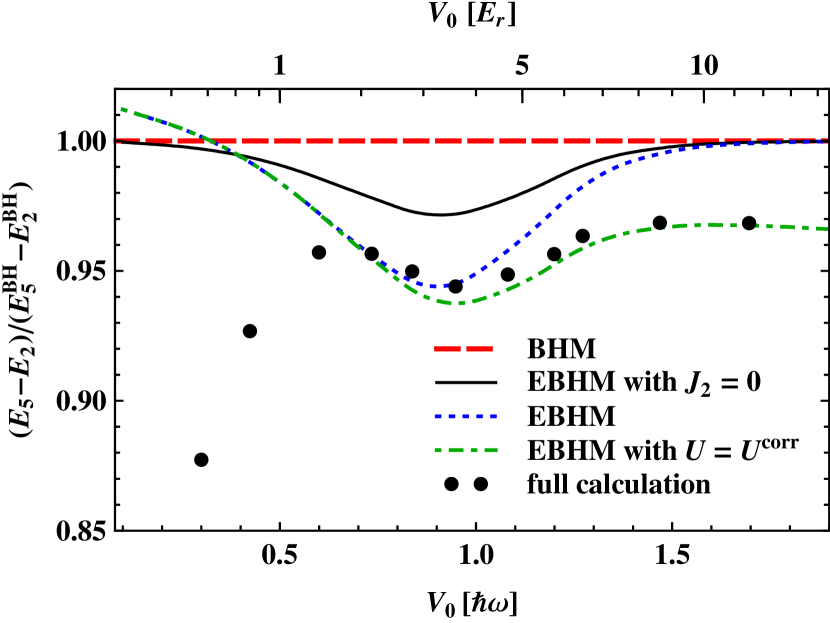
Figure 11: (Color online) Energy difference $E_{5}-E_{2}$ in different orders of approximation as a function of the lattice depth $V_{0}$ for $a_{\rm sc}\approx-180a_{0}$. The value of $E_{5}-E_{2}$ is shown relative to the same energy difference predicted by the BHM in BH representation. The BH representation of $\epsilon_{0},\epsilon_{\rm\pm 1}$ was determined for $k_{0}x_{B}=3\pi/2$ and the value of $J$ and $J_{2}$ for $k_{0}x_{B}=2\pi$.

In Fig. 11 $E_{5}-E_{2}$ is shown relative to its value for the BHM with parameters steming from the BH representation. The correct energy difference is compared to the one predicted by the BHM which is successively amended. First, only effects of NN interaction are incorporated by the use of the EBHM without NtNN hopping (i. e. setting $J_{2}=0$). Then the full EBHM is considered which is finally corrected by replacing $U^{\rm BH}$ by $U^{\rm corr}$. The relative importance of these three corrections for different lattice depths becomes clearly visible. Due to the weakness of the interaction NtNN hopping and NN interaction have comparable influence, most dominant at $V_{0}\approx 0.9\,\hbar\omega$. For deeper lattices the correction of the interaction parameter becomes increasingly important and dominates finally for $V_{0}>1.3\,\hbar\omega$ the correction of the BHM.

By including all three corrections one is able to determine the correct energy difference with about 1% accuracy down to lattice depths of only $V_{0}=0.7\,\hbar\omega$. Below this lattice depth the EBHM is unable to improve the BHM significantly. Additional effects steming from the confinement $\hat{V}_{\rm conf}$ finally dominate the properties of the energy spectrum and the description by a BHM or even an EBHM becomes inappropriate.

Also for other differences of eigenenergies the prediction of the EBHM improves the one of the BHM at least qualitatively (depending on the importance of $\Delta$). Only for differences involving the first energy level this is not the case. Since for attractive interaction (as shown in Fig. 11) particles in the ground state predominantely occupy the middle well, the energy difference to higher lying states, where also the outher wells are occupied, is particularly influenced by $\Delta$. The error in the determination of $\Delta$ can therefore dominate over improvements of the EBHM. We have verified that the failure of the EBHM to improve the BHM results for energy differences involving the ground-state energy $E_{1}$ does not occur, if repulsive interactions are considered.

V Conclusions

We have investigated the validity of the standard and an extended Bose-Hubbard model in a triple-well optical lattice. We defined the optimal Bose-Hubbard parameter set to be the one which reproduces best the eigenenergies of our full numerical calculations. This allowed to determine when the Bose-Hubbard model is principally able to describe the system under consideration and whether corrections of the standard Bose-Hubbard parameters are needed.

For shallow optical lattices the confinement to three wells had a notable impact on the hopping parameter and the onsite energies. This impact could not be fully reflected by the standard values of these parameters. Disagreements due to the confinement vanished, however, for lattice depths $V_{0}$ larger than the ground-state energy of the harmonic approximation $1.5\,\hbar\omega$. Therefore, in this regime our results are valid for both large optical lattices and few-well systems. For results concerning the interaction parameter this is also true for shallower lattices, since this parameter is barely influenced by the confinement.

The standard interaction parameter showed to be valid only when the scattering length is smaller than one percent of the trap length. However, for this parameter we found an analytic expression which approximates the optimal interaction parameter very well for a large range of lattice depths and interaction strengths. Since its definition is quite general, one can expect that it is extendable to hetero-nuclear systems, interacting particles in different Bloch bands, and lattices with different wavelengths in the three spacial directions.

The error due to the neglect of the energy-dependence of the scattering length was quantified and found to be of less importance than effects caused by the incompleteness of the Wannier basis. For deep lattices this error is comparable to anharmonic effects.

Furthermore, we found that the sextic expansion of one well can already cover the full onsite interaction in the lattice. We have presented and explained the avoided crossing of repulsively bound pairs with states in higher Bloch bands. Finally, an extended Bose-Hubbard model was investigated and it was shown that in a region of small lattice depths it can partially improve the standard Bose-Hubbard model significantly.

References

- Hubbard (1963) J. Hubbard, Proc. R. Soc. London A 276, 238 (1963).
- Bloch et al. (2008) I. Bloch, J. Dalibard, and W. Zwerger, Rev. Mod. Phys. 80, 885 (2008).
- Jaksch et al. (1998) D. Jaksch, C. Bruder, J. I. Cirac, C. W. Gardiner, and P. Zoller, Phys. Rev. Lett. 81, 3108 (1998).
- Greiner et al. (2002) M. Greiner, O. Mandel, T. Esslinger, T. Hänsch, and I. Bloch, Nature 415, 39 (2002).
- Cramer et al. (2008) M. Cramer, C. M. Dawson, J. Eisert, and T. J. Osborne, Phys. Rev. Lett. 100, 030602 (2008).
- Valiente and Petrosyan (2008) M. Valiente and D. Petrosyan, J. Phys. B: At. Mol. Phys. 41, 161002 (2008).
- Winkler et al. (2006) K. Winkler, G. Thalhammer, F. Lang, R. Grimm, J. Hecker, Denschlag, A. J. Daley, A. Kantian, H. P. Büchler, and P. Zoller, Nature 441, 853 (2006).
- Fölling et al. (2007) S. Fölling, S. Trotzky, P. Cheinet, M. Feld, R. Saers, A. Widera, T. Müller, and I. Bloch, Nature 448, 1029 (2007).
- Cheinet et al. (2008) P. Cheinet, S. Trotzky, M. Feld, U. Schnorrberger, M. Moreno-Cardoner, S. Fölling, and I. Bloch, Phys. Rev. Lett. 101, 090404 (2008).
- Trotzky et al. (2008) S. Trotzky, P. Cheinet, S. Fölling, M. Feld, U. Schnorrberger, A. M. Rey, A. Polkovnikov, E. A. Demler, M. Lukin, and I. Bloch, Science 319, 5861 (2008).
- Stickney et al. (2007) J. A. Stickney, D. Z. Anderson, and A. A. Zozulya, Phys. Rev. A 75, 013608 (2007).
- Milburn et al. (1997) G. J. Milburn, J. Corney, E. M. Wright, and D. F. Walls, Phys. Rev. A 55, 4318 (1997).
- Anderlini et al. (2006) M. Anderlini, J. Sebby-Strabley, J. Kruse, J. V. Porto, and W. D. Phillips, J. Phys. B: At. Mol. Phys. 39, 199 (2006).
- Sebby-Strabley et al. (2006) J. Sebby-Strabley, M. Anderlini, P. S. Jessen, and J. V. Porto, Phys. Rev. A 73, 033605 (2006).
- (15) S. Grishkevich and A. Saenz, arXiv:0904.2504 (2009), (to be submitted).
- Tiesinga et al. (2000) E. Tiesinga, C. J. Williams, F. H. Mies, and P. S. Julienne, Phys. Rev. A 61, 063416 (2000).
- Stock et al. (2003) R. Stock, I. H. Deutsch, and E. L. Bolda, Phys. Rev. Lett. 91, 183201 (2003).
- Köhler et al. (2006) T. Köhler, K. Góral, and P. S. Julienne, Rev. Mod. Phys. 78, 1311 (2006).
- Mentink and Kokkelmans (2009) J. Mentink and S. Kokkelmans, Phys. Rev. A 79, 032709 (2009).
- Gross and Khaykovich (2008) N. Gross and L. Khaykovich, Phys. Rev. A 77, 023604 (2008).
- Slater (1952) J. C. Slater, Phys. Rev. 87, 807 (1952).
- Kohn (1959) W. Kohn, Phys. Rev. 115, 809 (1959).
- Jaksch and Zoller (2005) D. Jaksch and P. Zoller, Annals of Physics 315, 52 (2005).
- Busch et al. (1998) T. Busch, B.-G. Englert, K. Rzazewski, and M. Wilkens, Found. of Phys. 28, 549 (1998).
- Idziaszek and Calarco (2005) Z. Idziaszek and T. Calarco, Phys. Rev. A 71, 050701(R) (2005).
- Bolda et al. (2002) E. L. Bolda, E. Tiesinga, and P. S. Julienne, Phys. Rev. A 66, 013403 (2002).
- Gao (1998) B. Gao, Phys. Rev. A 58, 4222 (1998).
- Block and Holthaus (2002) M. Block and M. Holthaus, Phys. Rev. A 65, 052102 (2002).
- Blume and Greene (2002) D. Blume and C. H. Greene, Phys. Rev. A 65, 043613 (2002).
- Deuretzbacher et al. (2008) F. Deuretzbacher, K. Plassmeier, D. Pfannkuche, F. Werner, C. Ospelkaus, S. Ospelkaus, K. Sengstock, and K. Bongs, Phys. Rev. A 77, 032726 (2008).
- Mazzarella et al. (2006) G. Mazzarella, S. M. Giampaolo, and F. Illuminati, Phys. Rev. A 73, 013625 (2006).
- Boers et al. (2007) D. J. Boers, B. Goedeke, D. Hinrichs, and M. Holthaus, Phys. Rev. A 75, 063404 (2007).