Abstract

A retrospective historical overview of the phenomenon of spontaneous symmetry breaking (SSB) in quantum theory, the issue that has been implemented in particle physics in the form of the Higgs mechanism. The main items are:
– The Bogoliubov’s microscopical theory of superfluidity (1946);
– The BCS-Bogoliubov theory of superconductivity (1957);
– Superconductivity as a superfluidity of Cooper pairs (Bogoliubov - 1958);
– Transfer of the SSB into the QFT models (early 60s);
– The Higgs model triumph in the electro-weak theory (early 80s);
The role of the Higgs mechanism and its status in the current Standard Model is also touched upon.

1 Introduction

Spontaneous symmetry breaking is a well-established term in quantum theory; its essence is simple. One has in mind a physical system that can be described by expressions (Lagrangian, Hamiltonian, equations of motion) obeying some symmetry, while a real physical state of the system corresponding to some partial solution of the equations of motion does not obey this symmetry. One meets such a case when the lowest of possible symmetrical states does not provide the system with absolute energy minimum and turns out to be unstable. A particular lowest state is not unique; a full collection of them forms a symmetric set. The real cause of symmetry breaking and transition of the system to some of the lowest non-symmetrical states usually turns out to be an arbitrary small asymmetrical perturbation.

Figure 1:  Simple mechanical system illustrating  spontaneous symmetry breaking:  (a) initial state; (b) final state.

As a simple illustration take a system of an empty vessel with a convex bottom and a tiny massive ball. Let the vessel, which is a figure of revolution, stand vertically and the ball be located above it, just on the axis (Fig. 1 ). The system is symmetric with respect to rotation around the vertical axis. Let the ball fall down due to the force of gravity. Upon reaching the bottom, the ball will not stand at the center of convex surface and will roll down to some point at the periphery of the bottom (Fig.1 ). Thus, the initial conditions are symmetrical, while the final state is not.

A more pithy example is the magnetized ferromagnet. The compass was known to the ancient Chineses, but only in the beginning of XVIII century an Oxford professor of astronomy John Keill[1] noticed that heating destroys magnetic property :
“… if a Loadstone be put into the Fire, insomuch that the internal Structure of its Parts be changed or wholly destroyed, then it will lose all its former Virtue, and will scarce differ from other Stones.”

A systematical study of thermal properties of magnetic substances was undertaken by Pierre Curie, who discovered a sharp decrease of magnetization as the temperature approached the critical value, now called the Curie point. Above the critical temperature ferromagnetism disappears. With decreasing temperature from the critical point the direction of magnetization may be changed to the opposite one if a ferromagnetic is placed in the external field opposite to the reference direction of magnetization and then this field is removed. Thus, ferromagnetic magnetization is related with two important notions. First, it is spontaneous symmetry breaking, as the external field may be chosen as weak as one wishes. Second, the value of magnetization is just the quantity that was called the order parameter in the Landau theory of phase transitions [2] (see also pp 234-252 in [3]). This parameter is nonzero in the ferromagnetic region and continuously decreases to the critical point where it vanishes.

The main subject will be exposed on the material of quantum statistics (superfluidity and superconductivity) with a smooth transition to quantum field theory, as far as the recent upgrading of interest in Spontaneous Symmetry Breaking (SSB) stems from the quantum-field context. The previous contribution by Dremin, which plunged the audience in the bulk of technical details of future experiments at the Large Hadron Collider (LHC), reminded us of the  “Higgs expectations”. The latter are tightly related with SSB.

Incidentally, in our exposition, we will mention two diverse and partially opposing one another ways of conceiving main ideas on the structure of the physical world. That is the ways of constructing the physical theory.

The initial feeding material of our science, the data from observations, are to be systematized and understood. To put in order, one usually constructs a phenomenological model that is based on some physical idea, the model invested in a mathematical form, the form of a physical law. An important criterion of successfulness of the scheme and its grounds is not only a reasonable correlation of the initial data, but possibility prediction of new effects with a clear-cut way of their implementation. This is a usual road of a phenomenologist, the way “from a phenomenon to a theoretical scheme” and backwards.

Along with this, many important steps in the building of the physical theory are performed by another, a more speculative way. Remind Heraklit, unification of the celestial and terrestrial gravity, electricity and magnetism, as well as the recently discovered principle of  dynamics from symmetry  that made the foundation of the electro-weak theory and quantum chromodynamics.

Adherents to this way of thinking, the people that try to start from deep and profound ideas, from primary principles ab initio, are known as “reductionists”. In statistical physics the latter, as a rule, are adherents to a microscopical approach.

At the same time, the reductionists comprise an overwhelming majority of founders of basic fundamentals of modern physics like the theory of relativity, quantum mechanics and the theory of quantum fields.

Meanwhile, in our opinion, one should not exaggerate an opposition of these two modes of reflection. An important detail is that between equations, e.g., equations of classical mechanics or Maxwell equations in medium (plasma) and laws that describe a sequel of observed events for instance, laws of a planet motion or the Meissner law in a superconductor, there is a space, a logical gap. Just here the phenomenology works. Due to this, efforts of reductionists and phenomenologists, at the very end, supplement each other. Turn to examples.

In the early 30s, by heuristic reasonings, Fermi devised a four-fermionic Lagrangian for a weak nuclear force, initially with one coupling constant $G_{F}\,.$ The Fermi Lagrangian, with subsequent modifications, played an important role for understanding and regulating numerous data on lepton dynamics. The Fermi model modification of the mid50s included up to 10 coupling parameters.
More profound understanding of the weak interaction was achieved a quarter of a century later, in the Glashow–Salam–Weinberg (GSW) gauge theory of electro-weak interaction with its massive vector $W\,$ and $Z\,$ bosons that appeared to be a “missing link” transmitters of forces between lepton currents. The origin of heavy masses ($\sim 90\,$GeV) of these particles is connected with SSB. The GSW theory is elegant and rather simple, being based on the new general principle  “dynamics from symmetry”. A transition to a deeper level reduced greatly the number of parameters.

In the year of 1941, quite soon after the experimental discovery of superfluidity, Lev Davidovich Landau  “just on the move” as it Kapitsa said, devised a phenomenological model [6] (see also pp 352-385 in [3] and [7]) that described quite well some essential properties of HeII – thermodynamics, kinetics and so on.

The pith of the Landau’s reasoning was the assumption of the dominating role of the collective quantum effect. Analysis at the microscopic level appeared five years later as a model of a weakly imperfect Bose gas, when Nikolaj Nikolaevich Bogoliubov proposed to treat atoms of HeII as weakly repulsing particles interacting with condensate. Here the key element consisted in the admission of that the condensate contained a macroscopically large number of helium atoms. That was the hypothesis that led to the elucidation of the nature of the Landau collective effect. In his paper [8] (see also pp 108-112 in [5] and [9]), the famous $(u,v)\,$ transformation was introduced that is tightly related with spontaneous breaking of phase symmetry responsible for the conservation of the number of particles.

The third example, finally. The remarkable 1950 paper by Ginzburg and Landau[10] (see also pp 126-152 in [3]) – phenomenological description of the superconductivity by a specially devised, rather abstract, wave-like function $\Psi(\mathbf{r})\;$ (the two-component order parameter) of the collective of the superconducting electrons. However, the understanding of the function $\Psi(\mathbf{r})\;$ physical content appeared 8-9 years later, after elaborating the Bardin-Cooper-Schrieffer and, particularly, Bogoliubov microscopical constructions, explicitly taking into account the interaction of electrons with the ion lattice vibrations.

2 SSB in quantum statistics

2.1 Superfluidity

The theory of superfluidity is a good example of interconnection between phenomenological ideas and mathematical constructions. The original explanation of the phenomenon of superfluidity offered by Landau[6] was based on the idea that at low temperatures the properties of liquid ${\rm{}^{4}He}\,$ were defined by collective excitations (phonons) rather than a quadratic spectrum of individual particle excitations. It follows from this assumption that in moving with velocity not exceeding a certain critical value it is impossible to slow down the liquid by transferring energy and momentum from the wall to individual atoms because a linear form of the phonon spectrum does not allow one to obey simultaneously the laws of energy and momentum conservation. The need for agreement between the form of the spectrum and the thermodynamic properties of liquid helium motivated Landau to introduce particular excitations, in addition to phonons, with a quadratic spectrum beginning with a certain energy gap, excitation, which he called rotons.
Bogoliubov’s theory is based on a physical assumption that in weakly nonideal Bose gas there is a condensate akin to ideal Bose gas. The existence of the Bose condensate leads to a unique wave function of the whole system, i.e., collective effect. Therefore, the presence of even a weak interaction transforms single-particle excitations into the spectrum of collective excitations. To calculate this spectrum, Bogoliubov inferred that at low temperatures the Bose condensate contains a macroscopically large, of an order of Avogadro number $N_{A}\,,$ number of particles $N\,$ as a result of which matrix elements of the creation and annihilation operators of particles in the condensate are proportional to  “large”  number $\sim\sqrt{N_{0}}\,,$ and the main contribution to the system dynamics comes from the processes of particle transition from the condensate to the continuous spectrum and back to the condensate.

Following paper [8], we start with the second-quantized description of the system of Bose particles in the coordinate representation. The Hamiltonian of system with a pair interaction looks like

$$H=-\tfrac{\hbar^{2}}{2m}\int d\,x\,\Psi^{*}(x)\Delta\Psi(x)+\int d\,x\int d\,y\,\Psi^{*}(x)\Psi(x)\,V(x-y)\,\Psi^{*}(y)\Psi(y).$$ (1)

Extraction of the condensate corresponds to a transition of the $\Psi\,$ function to the sum

$$\Psi(x)=C+\phi(x)\,\quad\Psi^{*}(x)=C+\phi^{*}(x)$$ (2)

of the “large constant”  $C\,$ (containing an identity operator) and the  “small operator” $\phi(x)\,.$ Since the Fourier transform of the constant is the Dirac delta function, in the discrete momentum representation

$$\Psi(x)=\tfrac{1}{\sqrt{V}}\,\sum_{k}a_{k}\,e^{\tfrac{i\,(k\,x)}{\hbar}}\,\quad\phi(x)=\tfrac{1}{\sqrt{V}}\,\sum_{p\neq 0}\,b_{p}e^{\tfrac{i\,(p\,x)}{\hbar}},\,\quad\dots$$ (3)

one can write

$$a_{k}=a_{0}\,\delta_{k,0}\,c+\left[1-\delta_{k,0}\right]\,\delta_{k,p}\,b_{p}\,;\quad c=C/\sqrt{V}=\sqrt{N_{0}/V}\,,$$ (4)

where $a_{k}\,,a^{*}_{k}\,\,$ and $\,b_{p}\,,b_{p}^{*}\,$ are operators with Bose commutation relations

$$a_{k}\,a^{*}_{q}-a^{*}_{q}\,a_{k}=\delta_{k,q}\,;\quad b_{p}\,b^{*}_{l}-b^{*}_{l}\,b_{p}=\delta_{p,l}\,.$$

Under the assumption of the decisive role of the condensate one can neglect terms responsible for an interaction of above-condensate atoms with each other.

Then the total Hamiltonian of Bose gas in the momentum representation

$$H_{B_{0}}=\sum_{k}\,T(k)\,a^{+}_{k}\,a_{k}+\sum_{k,q}v(k_{1}-k_{2})\,a^{+}_{k_{1}}\,a_{k_{2}}\,a^{+}_{q_{1}}\,a_{q_{2}}\,\delta_{k_{1}-k_{2}\,,q_{1}-q_{2}}\,;\quad T(k)=\tfrac{k^{2}}{2m}\,,$$ (5)

with the Fourier transform $\,v(k)>0\,$ of the potential energy of weak pair repulsion of helium atoms results in the Bogoliubov Hamiltonian [8] of the weakly nonideal Bose gas model

$$H_{B_{0}}\to H_{0}+H_{B_{1}}\,;\quad H_{0}=v(0)\,{\mathbf{N}}_{0}^{2}/2V\,,\quad{\mathbf{N}}_{0}=a^{+}_{0}\,a_{0}\,,$$

where $\,{\mathbf{N}}_{0}=a^{+}_{0}\,a_{0}$ is the particle number operator (i.e., occupation number) in the condensate, and

$$H_{B_{1}}=\sum_{p\neq 0}\left\{T(p)+\frac{{\mathbf{N}}_{0}\,v(p)}{V}\right\}\,b^{+}_{p}b_{p}+\frac{1}{2V}\sum_{p\neq 0}v(p)\{b^{+}_{p}b^{+}_{-p}a_{0}a_{0}+a^{+}_{0}\,a^{+}_{0}\,b_{p}b_{-p}\}\,.$$ (6)

The second sum describes particle transitions from the condensate and back, i.e., production of pairs with zero total momentum from the condensate and their annihilation.

Bogoliubov’s next step rested on that the operators $a_{0}$ and $a^{+}_{0}$ of condensate atoms entered into the Hamiltonian in combination of $a_{0}/\sqrt{V}$ and $a^{+}_{0}/\sqrt{V}$ and within a large volume limit approximately commute with each other. At the same time, their matrix elements contain $\sqrt{N_{0}}\,.$ Therefore, the operators $a_{0}$ and $a^{+}_{0}$ can be treated as numbers $\,=\sqrt{N_{0}/V}\,,$ and the operator ${\mathbf{N}}_{0}\,,$ divided by $V\,,$ can be replaced by the finite density of Bose condensate $\rho_{0}=N_{0}/V\,.$ As a result, the Hamiltonian $H_{B_{1}}\,$ becomes a uniform bilinear form in operators with nonzero momentum

$$H_{B_{2}}=\sum_{p\neq 0}\left\{[T(p)+\rho_{0}\,v(p)]\,b^{+}_{p}b_{p}\,+\tfrac{\rho_{0}\,v(p)}{2}\left[b^{+}_{p}b^{+}_{-p}+\,b_{p}b_{-p}\right]\right\}\,.$$ (7)

It should be noted that the initial expression (5), like (6), is invariant with respect to phase transformation of the operators

$$a_{k}\to e^{i\phi}\,a_{k}\,,\quad a_{k}^{+}\to e^{-i\phi}\,a_{k}^{+}\,,$$ (8)

which corresponds to conservation of particle number. Indeed, the Hamiltonian $H_{B_{1}}\,,$ like $H_{B_{0}}\,,$ commutes with the operator of total particle number ${\mathbf{N}}=\sum_{k}\,a^{+}_{k}a_{k}\,.$ However, this property is not inherent in approximation $H_{B_{2}}\,$ that does not contain condensate operators. Just this step, i.e., a transition to the bilinear (exactly solvable) approximate Hamiltonian (7), leads to spontaneous symmetry breaking.

The diagonalization of the bilinear Hamiltonian $H_{B_{2}}\,$ is not a particular problem and can be accomplished by the famous Bogoliubov canonical $(u,v)$ transformation

$$b_{p}\to\xi_{p}=u_{p}b_{p}+v_{p}b_{-p}^{+}\,;\quad b^{+}_{p}\to\xi^{+}_{p}=u_{p}b^{+}_{p}+v_{p}b_{-p}\,;\quad u_{p}^{2}-v_{p}^{2}=1$$ (9)

with real coefficients  “braiding”  creation and annihilation operators. Thus, the new operators $\xi_{p}\,$ and $\xi_{p}^{+}\,$ are a superposition of the old ones. A  “hyperbolic rotation”  of operators (9) corresponds to a unitary transformation

$$b_{p}\to\xi_{p}=U^{-1}_{\alpha}b_{p}\,U_{\alpha}=u_{p}b_{p}+v_{p}b_{-p}^{+}\,;\quad U_{\alpha}=e^{\sum_{p}\alpha(p)\,[b_{p}^{+}b_{-p}^{+}-b_{p}b_{-p}]}\,,$$ (10)

where the coefficient $\alpha(p)$ depends on the parameters of the initial Hamiltonian. The transformed Hamiltonian is

$$H=\sum_{p\neq 0}E(p)\,\xi_{p}^{+}\,\xi_{p}$$ (11)

with the spectrum

$$E(p)=\sqrt{T^{2}(p)+T(p)\,v(p)\,\rho_{0}}\,.$$ (12)

The new ground state

$$\Psi_{0}(\alpha)=U_{\alpha}^{-1}\,\Phi_{0}=e^{-\sum_{p}\alpha(p)\,b_{p}^{+}b_{-p}^{+}}\,\Phi_{0}$$ (13)

includes superpositions of correlated pairs with the total zero momentum. Transformation (9), (10) leads to a spectrum of collective excitations (12). The dependence of energy on momentum has an initial linear part that is necessary for explanation of superfluidity and a nonlinear part with flexure that places Landau’s rotons into a required position (see Fig. 2[b])

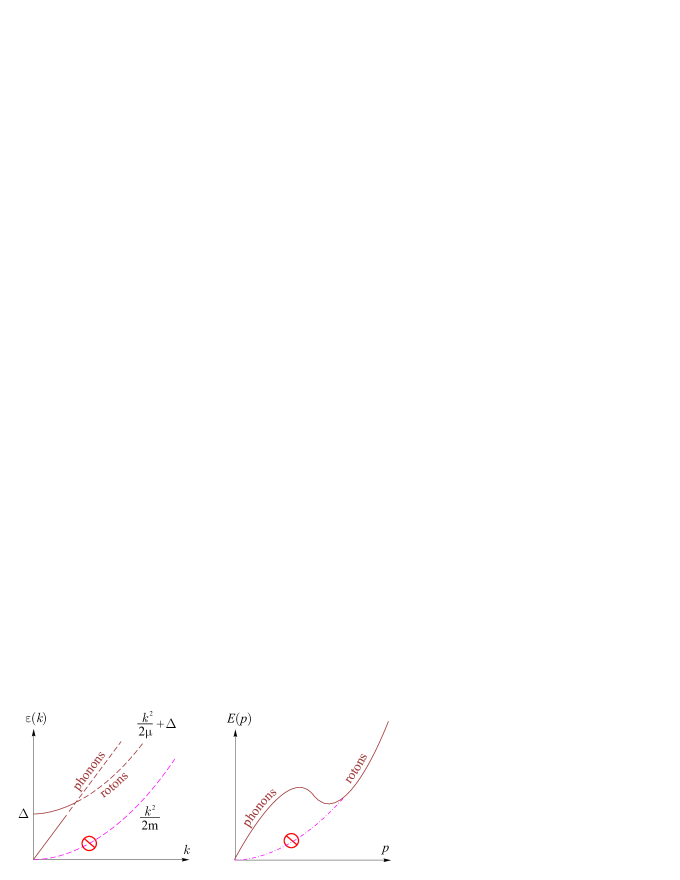
Figure 2: [a] Spectrum of phonons and rotons in the Landau phenomenological theory;  [b] The Bogoliubov-Landau spectrum of collective excitations following from the expression (12) of the Bogoliubov microscopic theory [8, 9].

The absence of single-particle excitations, like in a phenomenological approach, underlies the formulation of the model, though an operator form of a canonical transformation gives information about the nature of collective excitations and the structure of the new ground state (13).

As mentioned above, the initial Hamiltonian of weakly non-ideal Bose gas (5) is invariant with respect to gauge transformation (8) providing conservation of the total particle number $N\,.$ However, Bogoliubov’s bilinear Hamiltonian (7) has no this property, which corresponds to symmetry breaking. This Hamiltonian appeared as a result of the substitution of operator  “condensate”  contributions (at $k=0\,$)) by c-numbers. This substitution assumes nonzero values of vacuum averages $\langle a_{0}^{+}\rangle$ and $\langle a_{0}\rangle\,,$ that are connected with a transition to the new vacuum by the unitary operator

$$U_{c}=e^{c\,(a_{0}^{*}-a_{0})}\,,\quad a_{q}\to U_{c}^{-1}\,a_{q}\,U_{c}=b_{q}+c\,a_{0}\,.$$ (14)

2.2 Superconductivity

Another example of spontaneous symmetry breaking is the phenomenon of superconductivity where phase invariance violation occurs, as in the case of phase transition to a superfluid state. Though superconductivity was discovered in 1911, significantly earlier than ⁴He superfluidity, a theoretical insight into the phenomenon of superconductivity was gained much later than explanation of superfluidity. A breakthrough along this line was a phenomenological theory suggested by Ginzburg and Landau (G-L). In G-L theory [10] a superconducting state was described by an effective “wave function”  of superconducting electrons playing the role of a two-component order parameter

$$\Psi(\hbox{\bf r})=|\Psi({\bf r})|\,{\rm exp}[i\Phi({\bf r})]\,.$$ (15)

The equilibrium properties of a superconductor are defined there by a free energy functional depending on $\Psi({\bf r})\,$ and external magnetic field ${\bf B}({\bf r})$:

$$F(\Psi) = F_{n0}+\int d\,{\bf r}\left\{\frac{|{\bf B}|^{2}}{8\pi}+a|\Psi|^{2}+\frac{1}{2}b|\Psi|^{4}\right.$$ (16)

$$+ \left.\sum_{\alpha}\frac{1}{2m^{*}}\left|\left(-i\hbar\nabla_{\alpha}-\frac{q}{c}\,A_{\alpha}\right)\Psi({\bf r})\right|^{2}\right\}$$

where $\,F_{n0}$ is free energy in a normal state, ${\bf B}={\rm rot}\,{\bf A}\,,$ $\,q\,$ and $\,m^{*}$ are effective charge and mass of superconducting electrons. In the original paper, those were arbitrary parameters which on general physical grounds were put equal to electron charge and mass. Modulus of the order parameter (15) is proportional to the density of superconducting electrons $\,n_{s}\,,$ and its phase $\Phi({\bf r})$ defines a superconducting current

$$j_{\alpha}=\frac{q\hbar}{m^{*}}\,|\Psi|^{2}\nabla_{\alpha}\,\Phi({\bf r})\,.$$ (17)

The essential feature of the G-L theory is that at the temperature of a superconducting transition $T_{\rm c}$ the coefficient $\,a\sim(T-T_{\rm c})\,$ changes the sign, while the positive coefficient $\,b\,,$ the effective mass $m^{*}\,$ and charge $q\,$ are independent of temperature. In such a case, the G–L functional (16) describes a transition from a normal state with $\Psi=0$ to a superconducting one at $T=T_{\rm c}\,,$ at which a nonzero order parameter $\Psi\neq 0\,$ arises. In the absence of a magnetic field, there occurs a second order phase transition with the mean-field critical indices. In the framework of the G-L theory, the behavior of a superconductor in an external magnetic field, including the Abrikosov vortex lattice in second type superconductors, was successfully described [22]. At the same time, the nature of a superconducting transition remained unclear.

We will comment on the structure of a  “potential”  term in expression (16)

$$V(\varphi)=a\,\varphi^{2}+\tfrac{b}{2}\,\varphi^{4}\,,\quad\varphi=|\Psi|$$ (18)

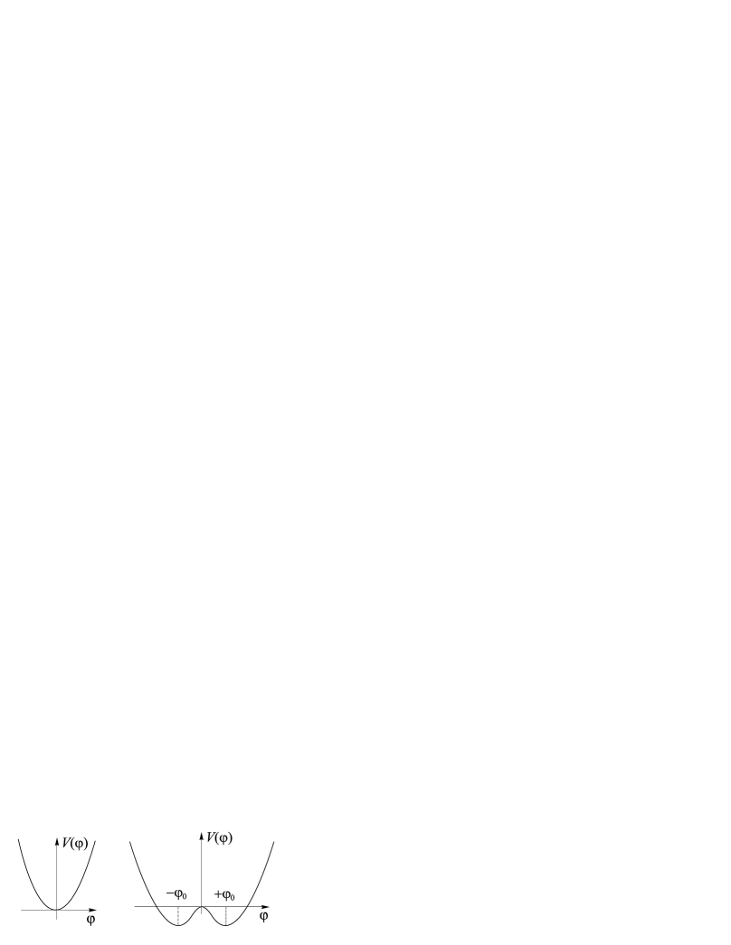
Figure 3: [a] Potential energy of the free scalar field with mass $m^{2}>0\,;$  [b] Potential function of the scalar field with self-interaction and unstable symmetric state.

in terms of a nonlinear (classical or quantum) oscillator. At $T>T_{\rm c}\,$ the coefficient $a\,$ is positive and can be expressed in terms of mass $a\to m^{2}/2\,.$ The first term dominates at small values of $\varphi\,$ and corresponds to an ordinary oscillator, like in Fig. 3[a]. Below the critical temperature this term is negative (see Fig. 3[b]) and the value $\varphi=0\,$ becomes unstable, which results in spontaneous breaking of discrete symmetry related to reflection $\varphi\to-\varphi\,.$ Equation (18) and illustrations in Fig 3 correspond to a one-component order parameter. To the two-component case there correspond illustrations in Fig. 1 describing violation of continuous symmetry of rotation.

The microscopic theory of superconductivity was developed only in 1957 by Bardeen, Cooper and Schiffer (BCS) [23, 24] and Bogoliubov[25, 26] (see also §2 in [27], [28] and pp 200-208 in [5]). BCS considered a simplified model in which an interaction of electrons due to an exchange of phonons was substituted for an effective attraction of electrons near the Fermi surface

$$H_{\rm BCS}=\sum_{{\bf k},\sigma}\,\varepsilon({\bf k})\,c^{\dagger}_{{\bf k}\sigma}c_{{\bf k}\sigma}+\sum_{{\bf k},{\bf k}{{}^{\prime}}}\,V_{{\bf k},{\bf k}{{}^{\prime}}}\,c^{\dagger}_{{\bf k}\uparrow}c^{\dagger}_{-{\bf k}\downarrow}c_{-{\bf k}{{}^{\prime}}\downarrow}c_{{\bf k}{{}^{\prime}}\uparrow}\,,$$ (19)

$$V_{{\bf k},{\bf k}^{{}^{\prime}}}=\left\{\begin{array}[]{ll}-{V_{\rm BCS}},&|\varepsilon({\bf k})-\varepsilon({\bf k}^{\prime})|<\omega_{ph}\\ 0,&|\varepsilon({\bf k})-\varepsilon({\bf k}^{\prime})|>\omega_{ph}\\ \end{array}\right\}\,,$$ (22)

where $\,c^{\dagger}_{{\bf k}\sigma}(c_{{\bf k}\sigma})\,$ are electron creation (annihilation) operators with momentum $\,{\bf k}\,$ and spin $\sigma=(\uparrow,\downarrow)=(+1/2,-1/2)\,,$ obeying the Fermi anticommutation relations:

$$\,[c_{{\bf k}\sigma},c^{{\dagger}}_{{\bf k^{\prime}}\sigma^{\prime}}]_{+}=\delta_{{\bf k,k^{\prime}}}\delta_{\sigma,\sigma^{\prime}}\,.$$

The Bloch electron energy in the normal phase $\varepsilon({\bf k})\,$ is reckoned from the Fermi energy $E_{\rm F}$, so that near the Fermi surface $\,\varepsilon({\bf k})\approx{\bf v}_{\rm F}\cdot({\bf k-k}_{\rm F})\,$, where $\,{\bf v}_{\rm F}=\partial\varepsilon({\bf k})/\partial{\bf k}\,$ and $\,{\bf k}_{\rm F}\,$ are the Fermi velocity and momentum, respectively. The interaction constant $V_{\rm BCS}$ defines attraction of electrons near the Fermi surface in a narrow energy layer $\,\pm\omega_{ph}\,,$ where $\,\omega_{ph}\,$ is a specific phonon energy. A variational wave function was used for calculation of the ground state energy and the spectrum of electron excitations.

$$|\Psi{\rm BCS}\rangle=\prod_{{\bf k}}\left[\sqrt{1-h_{\bf k}}+\sqrt{h_{\bf k}}\,c^{\dagger}_{{\bf k}\uparrow}\,c^{\dagger}_{-{\bf k}\downarrow}\right]\,|\Phi_{0}\rangle\,,\quad c_{{\bf k}\sigma}\,|\Phi_{0}\rangle=0\,,$$ (23)

where the variational parameter $h_{\bf k}],$ was determined from minimum of the ground state energy $\,W_{0}=\langle\Psi_{\rm\scriptsize BCS}|H_{\rm BCS}|\Psi_{\rm BCS}\rangle\,.$ It was established that an energy gap appears in the superconducting phase in the spectrum of one-electron excitations

$$\Delta\sim e^{-1/\lambda}\,;\quad E({\bf k})=\sqrt{\varepsilon^{2}({\bf k})+|\Delta|^{2}}\,,$$

where the coupling constant $\lambda=V_{\rm BCS}\,N(0)\,$ is determined by the effective interaction from Hamiltonian (19) and the density of electron states on the Fermi surface $N(0)\,.$ The thermodynamics and electrodynamics of a superconductor were considered, the temperature of a superconducting transition $\,T_{c}=1.14\,\omega_{ph}\,\exp\left(-1/\lambda\right)$ was calculated, and a universal relation between the gap in the spectrum at zero temperature and the temperature of a superconducting transition $\,2\,\Delta_{0}=3.52\,T_{c}$ was obtained. The gap in the spectrum arises due to the formation of bound states of electron pairs with the opposite momenta and spins,  “Cooper pairs”. The corresponding vacuum expectation value

$$\langle c^{{\dagger}}_{{\bf k}\uparrow}c^{{\dagger}}_{{\bf-k}\downarrow}\rangle=\Psi({\bf k})=|\Psi({\bf k})|\exp[i\Phi({\bf k})]\,$$ (24)

represents an order parameter written in the form (15). This expression is explicitly related to the violation of phase (gauge) invariance

$$c^{{\dagger}}_{{\bf k}\uparrow}\rightarrow c^{{\dagger}}_{{\bf k}\uparrow}\exp(i\varphi),\quad\langle c^{{\dagger}}_{{\bf k}\uparrow}\,c^{{\dagger}}_{{\bf-k}\downarrow}\rangle\rightarrow\langle c^{{\dagger}}_{{\bf k}\uparrow}\,c^{{\dagger}}_{{\bf-k}\downarrow}\rangle\,\exp(i2\varphi)$$ (25)

as in the theory of superfluidity [8]. In this case, a long-range order in the superconducting phase is specified not only by the appearance of Cooper pairs, $\,|\langle c^{{\dagger}}_{{\bf k}\uparrow}\,c^{{\dagger}}_{{\bf-k}\downarrow}\rangle|\neq 0\,,$ but also by the fixation of the order parameter phase in the whole volume of a superconductor.

Based on the BCS semi-phenomenological theory, Gor’kov [29] gave a consistent derivation of the G-L functional (16) and showed that an effective charge corresponds to a Cooper pair, i.e., $q=2\,{\rm e}\,,$ and an effective mass should be taken equal to the mass of a Cooper pair $\;m^{*}=2\,m\,.$ In so doing, it is convenient to normalize the modulus of the order parameter to the density of superconducting electron pairs $\,|\Psi({\bf r})|^{2}=n_{s}/2.$

Before the appearance of a detailed BCS paper [24] Bogoliubov succeeded in constructing a microscopic theory of superconductivity for the original Fröhlich electron-phonon model

$$H_{\rm Fr}=\sum_{{\bf k},\sigma}\,\varepsilon({\bf k})\,c^{\dagger}_{{\bf k}\sigma}c_{{\bf k}\sigma}+\sum_{\bf q}\,\omega({\bf q})\,b^{\dagger}_{{\bf q}}b_{{\bf q}}+g_{Fr}\sum_{{\bf k},{\bf q},\sigma}\,\sqrt{\tfrac{\omega({\bf q})}{2V}}\,c^{\dagger}_{{\bf k}\sigma}c_{{\bf k+q}\sigma}(b^{\dagger}_{{\bf q}}+b_{-{\bf q}})\,,$$ (26)

where $\,\omega({\bf q})=s\,q\,,\,\,s\,$ is the velocity of sound, and the interaction of electrons with acoustic phonons is described by the Fröhlich coupling constant $\,g_{Fr}.$ Generalizing the method of canonical $(u,v)$ transformation from the theory of superfluidity [8, 9] Bogoliubov introduced new Fermi amplitudes $\alpha_{{\bf k},\sigma}\,,$ superpositions of electron creation and annihilation operators [25, 26] (see also §2 in [27]) :

$$\alpha_{{\bf k}\uparrow}=u_{k}\,c_{{\bf k}\uparrow}-v_{k}\,c^{{\dagger}}_{{-\bf k}\downarrow}\,\,,\quad\alpha_{{\bf k}\downarrow}=u_{k}\,c_{-{\bf k}\downarrow}+v_{k}\,c^{{\dagger}}_{{\bf k}\uparrow}\,\,;\quad u_{k}^{2}+v_{k}^{2}=1\,,$$ (27)

where $\,u_{k},\,v_{k}\,$ are real functions.

The new Fermi amplitudes $\,\alpha_{{\bf k}\sigma}\,$ and $\alpha^{{\dagger}}_{{\bf k}\sigma}\,$ were used to carry out compensation of the so-called  “dangerous diagrams”  responsible for the production of electron pairs with the opposite momenta and spins. In the Fermi amplitude representation (27) the Hamiltonian of electrons in a superconducting state takes the form of Hamiltonian of the quasiparticle ideal gas

$$H_{\rm Fr}\to H_{\rm B}=\sum_{{\bf k},\sigma}E({\bf k})\,\alpha^{{\dagger}}_{{\bf k}\sigma}\,\alpha_{{\bf k}\sigma}+U_{0},\quad E({\bf k})=\sqrt{\varepsilon^{2}({\bf k})+|\Delta({\bf k})|^{2}},$$ (28)

where the spectrum of excitations of quasiparticles $E({\bf k})$ is defined by the spectrum of electrons in the normal phase $\,\varepsilon({\bf k})\,$ and the gap in a superconducting state $\,\Delta({\bf k})\,$, depending on momentum k in the general case. The equations derived by Bogoliubov for the gap and the superconducting temperature coincide with those in the BCS theory with the intensity directly determined by the Fröehlich coupling constant in Hamiltonian (26): $\,\lambda=g_{Fr}^{2}\,N(0)\,$.

Bogoliubov’s quasiparticles (27) (sometimes called  “bogolons”) provide us with a clear physical picture of the spectrum of quasiparticle excitations as a superposition of a particle and a hole which have a gap in the spectrum on the Fermi surface. Let us give a spectral function of quasiparticle excitations in the superconducting phase

$$A_{sc}({\bf k},\omega)={u}_{\bf k}^{2}\,\delta(\omega-E_{\bf k})+{v}_{\bf k}^{2}\;\delta(\omega+E_{\bf k}),$$ (29)

with due account for the expressions derived by Bogoliubov for the coefficients in transformation (27):

$$u_{k}^{2}=\frac{1}{2}\left[1+\frac{\varepsilon({\bf}k)}{E({\bf k})}\right],\quad v_{k}^{2}=\frac{1}{2}\left[1-\frac{\varepsilon({\bf k})}{E({\bf k})}\right].$$

Away from the Fermi surface, $|\varepsilon({\bf k})|\gg|\Delta({\bf k})|,\;E({\bf k})\approx|\varepsilon({\bf k})|\,,$ quasiparticle excitations are either electrons outside the Fermi sphere for $\,\varepsilon({\bf}k)>0,\;u_{k}^{2}\approx 1,\,v_{k}^{2}\approx 0\,$, or holes inside the Fermi sphere for $\,\varepsilon({\bf}k)<0,\;u_{k}^{2}\approx 0,\,v_{k}^{2}\approx 1\,$. In the vicinity of the Fermi surface, $|\varepsilon({\bf k})|\ll|\Delta({\bf k})|,\;E({\bf k})\approx|\Delta({\bf k})|$, excitations are a coherent superposition of an electron and a hole, so that the spectral function (29) has two peaks with equal weights: $\,u_{k}^{2}\approx v_{k}^{2}\approx 1/2\,$. In this case, an energy gap for electron excitations equals $2|\Delta({\bf k})|\,.$ When passing to the normal phase, $\,|\Delta({\bf k})|=0\,,$ the spectral function takes a standard form $\,A_{n}({\bf k},\omega)=\delta(\omega-\varepsilon({\bf}k))\,$ with a linear spectrum of excitations near the Fermi surface: $\,\varepsilon({\bf k})\approx{\bf v}_{\rm F}\cdot({\bf k-k}_{\rm F})\,$. Figure 4 shows the spectral phase of quasiparticle excitations (29) two branches of which correspond to the spectrum $\,\omega=\pm\,E({\bf k})$ with the gap $|\Delta({\bf k})|$.

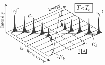
Figure 4: Spectral function of one-electron quasiparticel exitations (29) of the Bogoliubov theory [25] in supercunducting phase (taken from paper [30]).

A similar quasiparticle spectrum with two peaks was observed, for instance, in photoemission experiments in high-temperature superconductors [30]), which proves the coherent nature of quasiparticles in the superconducting phase.

Based on the Bogoliubov representation of quasiparticles it is easy to calculate thermodynamic and electrodynamic properties of a superconductor. The Bogoliubov canonical $(u,v)$ transformation (27) is widely used in solving present-day problems in the theory of superconductivity.

Noteworthy also is the generalization of the $(u,v)$ transformation to the case of inhomogeneous systems, the Bogoliubov – De Gennes transformation (see, e.g., [31]) that can be written in terms of coordinate-dependent $(u({\bf r}),v({\bf r}))$ wave functions of electrons in the superconducting phase. Though the results obtained on the basis of the BCS simplified model Hamiltonian (19) were impressive, the problem of accuracy of the obtained solutions still remained unsolved. Omitting the details we should like to note that further analysis [32] (also pp 168-176 in [5]) showed that the superconducting phase represents a condensate of Cooper pairs (i.e., bosons) consisting of  “attracted”  electrons. The spectrum of excitations of a pair condensate satisfies the criterion of Landau’s superfluidity. Thus, Bogoliubov came to the conclusion of the unity of these two phenomena: it is superfluidity of Cooper pairs that creates a superconducting current. It should be pointed out that the identity of both these phenomena has recently been confirmed directly in experiments with ultracold fermion gases (see recent reviews [34, 35]).

Summing up the discussions of phase transitions in quantum statistics we should like to emphasize that in passing to the superfluid and superconducting state there occurs system’s spontaneous symmetry breaking, namely, phase (otherwise gauge) invariance.

3 SSB in quantum field theory

3.1 The 1960 events

First attempts to use the SSB mechanism in QFT arose in the year of 1960. At that time, this idea was as if in the air. Almost concurrently there appeared several investigations within two-dimensional (1+1) QFT models. The very first ones submitted for publication were papers by Vaks and Larkin [36] (also p 873 in [37]). More or less simultaneously, the first results by Tavkhelidze and Nambu [38] were obtained. That summer Bogoliubov and Nambu met in Utrecht, as well as three months later in Rochester at HEP Conference. There, Nambu delivered a draft of his first paper with Jona-Lasinio [40]. In the comment to the Nambu talk Bogoliubov said (see page 865 in [37])

… one of my collaborators (Tavkelidze) has considered a Thirring–type one-dimensional model in which massless fermions interact with massive bosons. His calculations are not based on the self-consistent principle but on the ordinary Feynman diagram approach. The result is that there is a degeneracy in such a simple case.

All the QFT models in the early papers [36] – [40] of 1960, including the most well-known second paper by Nambu and Jona-Lasinio [41], were non-renormalizable, the results being dependent on cutoff. This drawback was avoided only by Arbuzov, Tavkhelidze and Faustov[42] (see also pp 527-530 in [43]).

The first successive use of the SSB took place several years later in the realistic model of electro-weak interaction by Glashow, Salam and Weinberg (GSW) where heavy gauge vector $W$ and $Z$ bosons acquire masses due to the Higgs mechanism.

3.2 The Higgs mechanism in Standard Model

Lagrangian of the complex (pseudo)scalar field with quartic self-interaction

$$L(\varphi,g)=\frac{1}{2}\,\left(\partial_{\mu}\varphi\right)^{2}-V(\varphi),\quad V(\varphi)=\frac{m^{2}}{2}\,\varphi^{2}+g\,\varphi^{4};\quad g>0$$

and stable lower state at $\varphi=0\,$ differs from Lagrangian of (two-component) Higgs field

$$V_{\rm Higgs}(\Phi^{2})=\lambda\left(\mathbf{\Phi}(x)^{2}-\Phi^{2}_{0}\right)^{2}\,;\quad\mathbf{\Phi}^{2}=\Phi^{2}_{1}+\Phi^{2}_{2}\,;\quad\Phi^{2}_{0}=\mbox{\small const.}$$ (30)

by the sign of quadratic term.

This corresponds to pure imaginary initial mass $\mu^{2}_{\rm H}=-4\lambda\,\Phi^{2}_{0}\,.$ After the shift $\Phi_{1}(x)\to\varphi_{1}(x)=\Phi_{1}(x)-\Phi_{0}\,$ by a constant $\Phi_{0}\,$ there arises the physical mass of the Higgs field

$$m_{\rm Higgs}=2\sqrt{2\lambda}\,\Phi_{0}\,,$$ (31)

proportional to the vacuum expectation value $\Phi_{0}\,.$

The main reason of this formal trick is the providing of nonzero masses to quanta of the above-mentioned gauge vector fields and to leptons and quarks. The first ones are expressed in terms of the coupling constants of the electro-weak interaction and $\Phi_{0}\,,$ like, e.g., $M_{Z}=(e\,\sqrt{2}\,\Phi_{0})/\sin 2\theta_{W}\,,$ while the last ones – via $\Phi_{0}\,$ and some Yukawa couplings. The Yukawa interactions involved are  especially added  to Lagrangian of the Standard Model for this and only this ! purpose. These Yukawa interactions after the shift by $\Phi_{0}\,$

$$g_{i}\bar{\psi}_{i}\,\Phi(x)\,\psi_{i}\to g_{i}\bar{\psi_{i}}\,\varphi(x)\,\psi_{i}+m_{i}\,\bar{\psi_{i}}\,\psi_{i};\,\quad m_{i}=g_{i}\,\Phi_{0}$$

provide masses for fermions.

This recipe, devoid of elegance, gives masses to leptons and quarks at the barter rule – one mass for one coupling constant. As a result, of ca 25 parameters (not counting neutrino masses) of the current Standard Model, just 12 are Yukawa constants, added  “by hand”.

Nevertheless, in the gauge sector of the SM, the SSB phenomenon implemented in the form of the Higgs model, led, about 40 years ago, to one of the greatest triumphs of QFT – prediction of the existence of neutral currents and numerical values of intermediate boson $W_{\pm}\,$ and $Z_{0}\,$ masses.

The 1979 Nobel Prize was awarded to theoreticians Glashow, Salam and Weinberg a few years before the experimental observation of $W_{\pm}\,$ and $Z_{0}\,$ particles, which, in its turn, was marked by another Nobel Prize in 1984.

Along with quantum electrodynamics and quantum chromodynamics, the GSW theory of electro-weak interactions stands for a splendid achievement of the human intellect. Being based upon an elegant and powerful principle  “dynamics from symmetry”, it forms a foundation of the Standard Model.

3.3 Search of Higgs boson

Meanwhile, the v.a.v. $\Phi_{0}\sim 250\,$ MeV, as defined from the electro-weak theory, is not sufficient for the estimation of the Higgs mass itself. Expression (31) for the mass value contains also the self-interaction coupling $\lambda\,$ that remains free. The current combination of theoretical and experimental restrictions results in a small window for possible mass value

114  GeV$\,<M_{\rm Higgs}<\ 154$  GeV,

that, hopefully, quite soon has to be studied at the Large Hadron Collider.

In the context of these  “great LHC expectations” it is worth reminding that a rather artificial Higgs construction (30) with its pure imaginary initial mass looks like a simple-minded relativistic replica of the Ginzburg–Landau classic functional (16), (18) with all its pragmatic advantages and physical shortcomings. The real underlying physical reason of SSB remains unknown, despite the electroweak theory success.

In such a situation, any aspirations for direct experimental observation, in our opinion, look unjustifiably straightforward.

4 Conclusion

4.1 As regards practice of Nobel Committee on physics

Now a few words about the Nobel Prize awarding. The Committee on Physics is the Class for Physics of the Royal Swedish Academy consisting of six members. Just these Swedish Academicians take a decision along with the Alfred Nobel testament and taking into account opinions of the leading specialists, mainly the Nobel laureates community with its well-known specific features.

Remind a few well known incidents.

Piotr Kapitsa discovered superfluidity in 1937. All his outstanding results in the low-temperature physics were obtained in the late 30s as well. He happened to be lucky enough to survive until his early nineties, when they bethought of him, more than 40 years later. We all remember in what a desperate state after an accident Landau got his Prize.

Items of another kind.

The 1999 Prize to t’Hooft and Veltman. The renormalization of the non-Abelian vector field, which acquired mass due to symmetry breaking, was a physically important and mathematically intricate problem. Its masterly solution by a rather complicated combination of formal tricks formed a base of electro-weak theory in late 60s and, subsequently, in Quantum Chromodynamics. However, the contribution of three Russian theorists to this solution is, at least, of no less importance than that of the laureates. Everyone calculates matrix elements (in electro-weak and QCD) by the Feynman rules formulated by Faddeev and Popov and performs renormalization with due account of Slavnov’s identities.

Now the last case. It combines two important, but rather distinct from each other, elements of the Standard Model. Their junction seems rather deliberate. The first one, spontaneous symmetry breaking in the theory of quantum gauge fields, in the current context of the XXI century could be referred (a f t e r  the Higgs particle discovery) to the names of Nambu, Goldstone and Higgs. The second one – formal mixing of three lepton generations (via Cabbibo-Kobayashi-Maskawa matrix) in the current version of the Standard Model – lies completely outside our scope.

4.2 Summary

Above, we attempted, in the fairy-tale form, to trace the development of a topical issue, spontaneous symmetry breaking, in the field of quantum physics during the XX century.

It is evident that the “Nobel race” is won by pragmatic theorists of the phenomenological kind, in terms of the introductory discussion. And this is natural, in a sense. Just in this mood [ ] the inventor of dynamite formulated the priority of benefit for people. A really clear-cut implementation of this spirit of the Nobel testament was the 2007 Prize in physics.

Meanwhile, the reductionists have no reasons to be dejected and envy. Their efforts’ reward lies in other fields. Thanks to their achievements, a more complete picture of the physical universe appears; ties of affinity are established between unrelated, at first sight, phenomena such as between electromagnetic and nuclear forces and, quite hopefully, between dynamics of the Universe evolution and some hypothetic generalization of the Standard Model (with additional space dimensions).

The author is indebted to Prof. Oleg Rudenko for the impetus of this talk and paper and continuous moral support. In the course of implementation of the initial plan, two mighty figures of Landau and Bogoliubov and complementary interference of their creative methods came to the fore. By a lucky chance, this paper is published just between their centennial jubilees.

The role of Drs. N.M. Plakida and V.B. Priezzhev in composing Section 2 is indispensable. Practically, they are coauthors of it. Besides, they provided the author with a lot of subtle comments along the whole text. It was a pleasure to follow essential advices of Dr. V.A. Zagrebnov as well. This investigation was supported in part by the presidental grant Scientific School–1027.2008.2.

References

- [1] John Keill, “Introduction to Natural philosophy”, 1726 ; republished by Kessinger Publ. (2003).
- [2] Landau L.D., Phys.Zc.Sowjet. 11, 26 (1937); also pp 234-252 in [3]
- [3] Landau L.D., Sobranie trudov . Nauka 1969, v.1 (in Russian)
- [4] Bogoliubov N.N., Vestnik AN SSSR, No.8, 36 (Aug 1958)[20 VI 1958]; pp 297-309 in [5] – in Russian.
- [5] Bogoliubov N N, Collection of scientific works,in 12 volumes, vol VIII, Moskva, Nauka 2008 – in Russian
- [6] Landau L.D., J.Phys.USSR, 5, 71 (1941);
- [7] Landau L.D., Sov.Phys.Usp. 97, 495 (1967).
- [8] Bogoliubov N.N., Journ. Phys.(USSR) 11, 23-32 (1947) [Submitted 12 X 1946] 171717In square brackets stands the date of submission, in parentheses – date of publication.;
- [9] Bogoliubov N.N., Sov.Phys.Uspekhi 97, 552 (1967).
- [10] Ginzburg V.L., Landau L.D., JETP 20, 1064 (1950);
- [11] Landau L.D., Sobranie trudov . Nauka 1969, v.2 (in Russian). English translation: L.D. Landau, Collected papers, Oxford, Pergamon Press (1965), p. 546].
- [12] P.C Hohenberg and Platzman, Phys.Rev. 152,198 (1966);
- [13] A.Aleksandrov et al Sov Phys JETP 41 915-918 (1975)
- [14] M.H. Anderson, et al. Science 269, 198 (1995).
- [15] Weinberg S, CERN Courier Jan/Feb 2008, 17-21.
-
[16]
Nobel press release 2008 “Broken Symmetries”:
http://nobelprize.org/nobel_prizes/physics/laureates/2008/phyadv08.pdf. - [17] N N Bogoliubov and D V Shirkov, “Quantum Fields”, Benjamin/Cummings, Reading, 1983.
- [18] Horace P. Yuen, Phys.Rev.A 13, 2226 - 2243 (1976)
- [19] Landau L D, J.Phys.(USSR), 11, 91-92 (1947) [15 XI 1946].
- [20] Landau L.D., Doklady AN SSSR 61, 253 [15 VI 1948] (1948);
- [21] Landau L.D.,Phys.Rev. 75, 884 [19 XI 1948] (1949);
- [22] Abrikosov A.A, Sov. Phys. JETP 5, 1174).
- [23] Bardeen J, Cooper L N, Schrieffer J R,Phys. Rev. 108, 162 (1 April, 1957).
- [24] Bardeen J, Cooper L N, Schrieffer J R, ibid. 108, 1175 (1 Dec,1957).
- [25] Bogoliubov N N, Sov.Phys.JETP 7 41-46, [10 X 1957] (1958);
- [26] Bogoliubov N N, Nuovo Cim. 7, 794 [14 XI 1957] (1958)
- [27] N N Bogoliubov, V.V. Tolmachev and D V Shirkov, “New method in the Theory of Superconductivity” Consult.Bureau, Inc., N.Y., Chapman & Hall Ltd., London, 1959.
- [28] N N Bogoliubov, Sov.Phys.JETP 7 51-54 [10 X 1957] (1958)
- [29] Gorkov L.P. Sov.Phys.JETP 36(9), 1364 (1959).
- [30] Matsui, H., et al., Phys. Rev. Lett. (2003) 90 217002.
- [31] De Gennes P G, Superconductivity of metals and alloys, W.A. Benjamin, Inc., New York - Amsterdam, 1966.
- [32] N N Bogoliubov, Zubarev D N, Tserkovnikov Yu A Doklady AN SSSR 117, 788 (1957) – in Russian
- [33] Bogoliubov N N, Vestnik AN SSSR, No.4, 25 (April 1958). – in Russian
- [34] Bloch I, Dalibard J, Zwerger W, Rev.Mod.Phys.80,885-964 (2008)
- [35] Giorgini S, Pitaevskii L P, Zwerger W, Rev.Mod.Phys. 80,1215-1274 (2008)
- [36] Vaks V.G., Larkin A.I., JETP 13, 192 (1961) [28 VIII 1960]
- [37] Proc. 1960 Intern.Conf. on HEP at Rochester, Intersc.Pub., N.Y. 1960.
- [38] Nambu Y, Report on Midwest Conf Theor Phys at Purdue “A Superconductor” Model… (1960); reprinted in Internat’l J.Mod.Phys.A 23 4063-4079 (2008).
- [39] Bogoliubov N N, Physica Suppl. 26 p.S1-S16 (1960); (Proc. Internt’l Congress Many-Particle Problems, Utrecht, June 1960)
- [40] Nambu Y and Jona-Lasinio G, Phys.Rev. 122, 345 (1961) [ 27 X 1960 ]
- [41] Nambu Y and Jona-Lasinio G, Phys.Rev.124, 246 (1961) [ 10 V 1961].
- [42] Arbuzov B.A., Tavkhedidze A.N. and Faustov R.N., Sov. Phys.Doklady 6 (1962) 598.
- [43] Bogoliubov N N, Collection of scientific works.in 12 volumes, vol IX, Moskva, Nauka 2008 – in Russian