Polarization studies on the two–step radiative recombination of highly–charged, heavy ions

Abstract

The radiative recombination of a free electron into an excited state of a bare, high–$Z$ ion is studied, together with its subsequent decay, within the framework of the density matrix theory and Dirac’s relativistic equation. Special attention is paid to the polarization and angular correlations between the recombination and the decay photons. In order to perform a systematic analysis of these correlations the general expression for the double–differential recombination cross section is obtained by making use of the resonance approximation. Based on this expression, detailed computations for the linear polarization of x–ray photons emitted in the (e, 2$\gamma$) two–step recombination of uranium ions U⁹²⁺ are carried out for a wide range of projectile energies.

1 Introduction

Radiative recombination (RR) is one of the basic processes that occurs in many stellar and laboratory plasmas as well as in collisions of heavy ions with electrons at ion storage rings and electron beam ion traps (EBIT). In this process, a free (or quasi–free) electron is captured into a bound state of an ion under the simultaneous emission of a photon. Because of their practical importance, detailed RR studies have been carried out during the last two decades for many elements and for a wide range of collision energies. At the GSI storage ring in Darmstadt, for example, a large number of experiments have been done for the electron capture into bare high–$Z$ ions, giving rise to hydrogen–like ions after the recombination has taken place [1, 2, 3, 4]. In the earlier experiments, the total and angle–differential cross sections have been measured hereby mainly for the ground–state capture and were found in good agreement with computations based on Dirac’s equation [5, 6, 7, 8, 9, 10, 11, 12, 13]. Apart from the RR into the $1s_{1/2}$ ground state, most recent studies have dealt also with the electron capture into the excited ionic states which later decay under the emission of one (or several) characteristic photons [14, 15, 16]. Such a subsequent decay is characterized (apart from the well known energies) by its angular distribution and polarization of the emitted photons. Both of these properties are closely related to the magnetic sublevel population of the excited ion as it arises from the electron capture. Several experiments have been carried out during last few years in order to study the angular distribution and linear polarization of the subsequent photons and, hence, enabled one to derive the alignment of the residual ions. For the capture of an electron into the $2p_{3/2}$ state of a bare uranium ion, for instance, a strong alignment was found especially for the residual ions, both by experiment [3] and in computations [15].

In most experiments on the radiative decay cascades of high–$Z$ ions, that were performed so far, the emission of the first, recombination photon remained unobserved. Although some insight about the collisional dynamics and electronic structure of heavy ions can be gained already from such an individual analysis of the characteristic radiation, more information is obtained, if both, the recombination and decay photons are measured in coincidence. Moreover, such photon–photon coincidence studies may have a significant impact also for the development of novel experimental methods and techniques. It was recently argued, for example, that they may help to determine the polarization properties of heavy ions beams [17], a request which has been recently made by several groups. Information about the ion polarization is required for studying, for example, the parity non–conservation (PNC) effects in highly–charged ions or in heavy–ion collisions [18, 19].

Despite of the importance of coincidence RR experiments for the forthcoming heavy ion research, little attention was paid up to now to their theoretical foundation. A first step towards the theoretical description of the $(e,2\gamma)$ RR process has been done only recently by us in Ref. [16]. In that paper, we have investigated the angle–angle correlations between the recombination and the subsequent decay photons, assuming that the polarization state of the photons remain unobserved. Owing to the recent advances in x–ray polarization techniques [20, 21], however, a polarization–resolved analysis of the correlated photon emission might become feasible in the next few years.

In this contribution, we study here the polarization correlations between the recombination and the subsequent decay photons in the $(e,2\gamma)$ radiative recombination of bare, high–$Z$ ions. These correlations can be described most easily in the framework of the density matrix theory, based on Dirac’s relativistic equation. However, before we shall present details from this theory, we first summarize in Section 2 the geometry under which the photon–photon polarization correlations are to be considered. In section 3, then, we make use of the resonance approximation in order to derive the general expression for the double–differential RR cross section which depends on the emission angles and the polarization states of both photons. Starting from this cross section, we perform in Section 3.4 a theoretical analysis for two selected scenarios of possible x–x coincidence studies. First, we shall discuss the angle–polarization correlation in which the linear polarization of the characteristic radiation is explored, while the spin states of recombination photons remain unobserved. Vice versa, the angular distribution of the characteristic decay photons, following the emission of linearly polarized RR photons, is discussed as a second scenario, then called the polarization–angle case. While, of course, the derived correlation functions can be applied to all hydrogen–like ions, detailed computations have been carried out for the electron capture into the $2p_{3/2}$ state of initially bare uranium ion, and along with its subsequent Lyman–$\alpha_{1}$ ($2p_{3/2}\to 1s_{1/2}$) decay. Results of our calculations are presented in Section 4 and indicate strong correlations between the angular and polarization properties of the recombination and decay photons. Finally, a brief summary is given in Section 5.

Relativistic units $\hbar=m_{e}=c=1$ are used throughout the paper unless stated otherwise.

2 Geometry of the two-photon radiative recombination

In order to explore the polarization correlations in the two–step radiative recombination of (finally) hydrogen–like ions, we shall first agree about the geometry under which the emission of both, the recombination and decay photons is observed. In the present work, the angular– and polarization–resolved properties of the photons will be analyzed in the projectile frame (i.e. the rest frame of the ion). Since in this frame the only preferred direction of the overall system is given by the electron momentum, here we adopt the quantization axis ($z$–axis) along the direction of the incoming electron (as seen by the ion). Together with the wave vector of the first photon $\bm{k}_{1}\equiv\bm{k}_{RR}$, this axis then defines also the reaction plane (x–z plane). Thus, only one polar angle $\theta_{1}\equiv\theta_{RR}$ is required to characterize the first, recombination photon, while the two angles $(\theta_{2},\phi_{2})$ are used for describing the emission of the subsequent decay photon (cf. Fig. 1).

Figure 1: Geometry (in the ion rest frame) for the radiative recombination of a free electron into an excited state of a bare projectile ion, and followed by a subsequent photon decay. The unit vectors of the linear polarization of the recombination and decay photons are defined in the planes that are perpendicular to the photon momenta $\bm{k}_{1}\equiv\bm{k}_{RR}$ and $\bm{k}_{2}\equiv\bm{k}_{dec}$, respectively.

For the theoretical analysis below we have to account for not only the emission angles but also the linear polarization vectors $\bm{\epsilon}_{1}$ and $\bm{\epsilon}_{2}$ of the recombination and decay photons. As usual, these vectors are defined in the planes that are perpendicular to the photon momenta $\bm{k}_{1}$ and $\bm{k}_{2}$ and are characterized by the angles $\chi_{1}$ and $\chi_{2}$ with respect to the planes as spanned by the quantization axis and the unit vectors $\hat{\bm{k}}_{1}$ and $\hat{\bm{k}}_{2}$, respectively.

3 Theoretical background

3.1 Resonance approximation

Having defined the geometry of the two–step radiative recombination, we are prepared now to derive expression for the differential cross section (DCS) of the process. The evaluation of such cross sections is usually traced back to the RR transition amplitude which, to zeroth order, is described by the diagram shown in Fig. 2. In this diagram, $p_{i}=(p^{0}_{i},\mathbf{p_{i}})$ and $\mu_{i}$ are the asymptotic four–momentum and the spin projection of the incoming electron, and $k_{1,2}=(k^{0}_{1,2},\mathbf{k_{1,2}})$ denote the four-momenta of the first (recombination) and second (decay) photon, respectively. By assuming that—for a given energy of the incoming electrons—the x–ray detectors observe only those photons which are emitted in course of (i) the electron capture into some (excited) ionic state $\left|n_{d}j_{d}\mu_{d}\right\rangle$ and (ii) the $\left|n_{d}j_{d}\mu_{d}\right\rangle\to\left|n_{b}j_{b}\mu_{b}\right\rangle$ subsequent decay to the ground state, we may restrict our theoretical analysis to the resonance approximation (cf. Ref. [8] for further details). Within such an approximation, the differential RR cross section reads as:

$$d\sigma = \frac{(2\pi)^{4}}{v_{i}}\left|\sum_{\mu_{d}}\frac{\left\langle n_{b}j_{b}\mu_{b}\left|e\alpha^{\nu}A^{\ast}_{2,\nu}\right|n_{d}j_{d}\mu_{d}\right\rangle\left\langle n_{d}j_{d}\mu_{d}\left|e\alpha^{\mu}A^{\ast}_{1,\mu}\right|p_{i}\mu_{i}\right\rangle}{\varepsilon_{b}+k^{0}_{2}-\varepsilon_{d}+i\frac{\Gamma_{d}}{2}}\right|^{2}$$ (1)

$$\times (p^{0}_{i}-k^{0}_{2}-\varepsilon_{b})^{2}(\mathrm{k}_{2}^{0})^{2}\,\rm{d}k^{0}_{2}\,\rm{d}\mathbf{\Omega}_{1}\,\rm{d}\mathbf{\Omega}_{2}\,,$$

where $\varepsilon_{d}$ and $\Gamma_{d}$ are the energy and the width of the intermediate (excited) state, $\varepsilon_{b}$ is the ground–state energy, $v_{i}$ denotes the velocity of the incident electron in the projectile frame and $\alpha^{\nu}=(1,\mbox{\boldmath$\alpha$})$ with $\mbox{\boldmath$\alpha$}=(\alpha_{x},\,\alpha_{y},\,\alpha_{z})$ being the vector of Dirac matrices. In Eq. (1), moreover, the interaction of the electron with the radiation field is characterized by the operator $e\alpha^{\nu}A_{\nu}^{*}=-e\mbox{\boldmath$\alpha$}\cdot\mathbf{A}^{*}$ where the vector potential [22]

$$\mathbf{A}(\mathbf{r})=\frac{\mbox{\boldmath$\epsilon$}\exp(\mathrm{i}\mathbf{k}\cdot\mathbf{r})}{\sqrt{2k^{0}(2\pi)^{3}}}\,,$$ (2)

describes the plane photon wave with polarization $\bm{\epsilon}$ and energy $k^{0}=|\mathbf{k}|=\omega$.

Owing to the energy conservation

$$k_{1}^{0}=p_{i}^{0}-\varepsilon_{b}-k_{2}^{0}\,,$$ (3)

only one of the photon energies can be varied independently. The radiative recombination cross section (1) is therefore differential in the angle and energy of the second photon but only with regard to the angle of the first photon. Moreover, if we assume the width $\Gamma_{d}$ of the intermediate excited state to be small compared to a distance to other states, we may extend the $k_{2}^{0}$ integration to the interval $(-\infty,\infty)$. Then by making use of the identity

$$\int\limits_{-\infty}^{\infty}\frac{dk^{0}_{2}}{\left(\varepsilon_{b}+k^{0}_{2}-\varepsilon_{d}\right)^{2}+\frac{\Gamma_{d}^{2}}{4}}=\frac{2\pi}{\Gamma_{d}}\,,$$ (4)

we can easily integrate Eq. (1) also over the energy of the second (decay) photon and finally obtain the double–differential RR cross section:

$$d\sigma=\frac{(2\pi)^{4}}{v_{i}}\,\frac{2\pi}{\Gamma_{d}}\,\omega^{2}_{1}\omega^{2}_{2}\,\left|\sum_{\mu_{d}}\left\langle n_{b}j_{b}\mu_{b}\left|R^{+}_{2}\right|n_{d}j_{d}\mu_{d}\right\rangle\left\langle n_{d}j_{d}\mu_{d}\left|R^{+}_{1}\right|p_{i}\mu_{i}\right\rangle\right|^{2}\rm{d}\mathbf{\Omega}_{1}\rm{d}\mathbf{\Omega}_{2}\,,$$ (5)

and where, for the sake of brevity, we have introduced the notation $R_{i}\equiv e\alpha^{\mu}A_{i,\mu}$ in order to denote the electron–photon interaction operator.

Figure 2: Feynman diagram for the two–step radiative recombination of a free electron with a bare nucleus. In this diagram, $p_{i}$ and $\mu_{i}$ are the four–momentum and spin projection of the incoming electron, $\left|n_{d}j_{d}\right\rangle$ and $\left|n_{b}j_{b}\right\rangle$ denote the intermediate and final (bound) hydrogenic states, and $k_{1,2}$ represent the four-momenta of the recombination and decay photons, respectively.

3.2 Alignment of excited ionic states

Equation (5) as derived in the previous Section enables one to analyze the angular and polarization correlations between the photons emitted in the two–step radiative recombination of (initially) bare ions. In order to perform such an analysis, it is useful to re–write the doubly–differential RR cross section as:

$$d\sigma = \frac{(2\pi)^{4}}{v_{i}}\frac{2\pi}{\Gamma_{d}}\omega^{2}_{1}\omega^{2}_{2}\sum_{\mu_{d}\mu^{{}^{\prime}}_{d}\mu_{b}}\left\langle n_{b}j_{b}\mu_{b}\left|R^{+}_{2}\right|n_{d}j_{d}\mu_{d}\right\rangle$$ (6)

$$\times \left\langle n_{d}j_{d}\mu^{\prime}_{d}\left|R_{2}\right|n_{b}j_{b}\mu_{b}\right\rangle\left\langle n_{d}j_{d}\mu_{d}\left|\rho^{(d)}\right|n_{d}j_{d}\mu^{\prime}_{d}\right\rangle\,\rm{d}\mathbf{\Omega}_{1}\rm{d}\mathbf{\Omega}_{2}\,,$$

where we assume that incoming electrons are unpolarized and that the spin state of the residual ion remains unobserved. In Eq. (6), moreover, we have introduced the density matrix of the intermediate ionic state:

$$\left\langle n_{d}j_{d}\mu_{d}\left|\rho^{(d)}\right|n_{d}j_{d}\mu^{\prime}_{d}\right\rangle=\frac{1}{2}\,\sum\limits_{\mu_{i}}\left\langle n_{d}j_{d}\mu_{d}\left|R^{+}_{1}\right|p_{i}\mu_{i}\right\rangle\left\langle p_{i}\mu_{i}\left|R_{1}\right|n_{d}j_{d}\mu^{\prime}_{d}\right\rangle\,.$$ (7)

This density matrix describes the magnetic sublevel population of the ion after the electron has been captured and the (first) RR photon has left the system along the direction $\hat{n}_{1}=(\theta_{1},\phi_{1})$. Instead of using the density matrix (7), however, it is often more convenient to represent the intermediate state of the ions in terms of the so–called statistical tensors $\rho_{kq}^{(d)}$. Although, from a mathematical viewpoint, the statistical tensors are equivalent to the density matrix, they are constructed to represent the spherical tensors of rank $k$ and component $q$ (cf. Refs. [16, 23, 24] for further details):

$$\rho_{kq}^{(d)}=\sum_{\mu_{d}\mu^{\prime}_{d}}(-1)^{j_{d}-\mu^{\prime}_{d}}C_{j_{d}\mu_{d},\,j_{d}-\mu^{\prime}_{d}}^{kq}\left\langle n_{d}j_{d}\mu_{d}\left|\rho^{(d)}\right|n_{d}j_{d}\mu^{\prime}_{d}\right\rangle\,,$$ (8)

where $C_{j_{d}\mu_{d},\,j_{d}-\mu^{\prime}_{d}}^{kq}$ denote the Clebsch–Gordan coefficients. Owing to the properties of these coefficients, the tensor components $\rho_{kq}^{(d)}$ are nonzero only for $0\leq k\leq 2j_{d}$ and $-k\leq q\leq k$.

In the theory of atomic collisions, the statistical tensors (8) are often re–normalized with respect to the zero–rank tensor [23, 24]

$$A^{(d)}_{kq}=\frac{\rho_{kq}^{(d)}}{\rho_{00}^{(d)}}\,.$$ (9)

These reduced tensors (or alignment parameters) are then independent on the particular normalization of the ion density matrix and are directly related to the relative population of the individual substates $\left|n_{d}j_{d}\mu_{d}\right\rangle$. By making use of these alignment parameters we may finally write the differential RR cross section as:

$$d\sigma = \frac{(2\pi)^{4}}{v_{i}}\frac{2\pi}{\Gamma_{d}}\omega^{2}_{1}\omega^{2}_{2}\,\rho_{00}^{(d)}\,\sum_{\mu_{d}\mu^{{}^{\prime}}_{d}\mu_{b}}\sum_{kq}(-1)^{j_{d}-\mu^{\prime}_{d}}C_{j_{d}\mu_{d},\,j_{d}-\mu^{\prime}_{d}}^{kq}A_{kq}^{(d)}$$ (10)

$$\times \left\langle n_{b}j_{b}\mu_{b}\left|R^{+}_{2}\right|n_{d}j_{d}\mu_{d}\right\rangle\left\langle n_{d}j_{d}\mu^{\prime}_{d}\left|R_{2}\right|n_{b}j_{b}\mu_{b}\right\rangle\rm{d}\mathbf{\Omega}_{1}\rm{d}\mathbf{\Omega}_{2}\,.$$

This cross section still depends on the polarization states and emission angles of both, the recombination and decay photons, because of the dependence of the reduced statistical tensors $A^{(d)}_{kq}=A^{(d)}_{kq}(\theta_{1},\phi_{1};{\bm{\epsilon}}_{1})$ as well as the bound–bound transition amplitudes $\left\langle n_{d}j_{d}\mu^{\prime}_{d}\left|R_{2}\right|n_{b}j_{b}\mu_{b}\right\rangle$ on the angular and polarization properties of the emitted (first and second-step) photons.

3.3 Evaluation of the free–bound and bound–bound transition amplitudes

As seen from Eqs. (8)–(10), any further analysis of the angular and polarization correlations between the recombination and subsequent decay photons can be traced back to the free–bound and bound–bound transition amplitudes, $\left\langle n_{d}j_{d}\mu_{d}\left|-e\bm{\alpha}\cdot\bm{A}\right|p_{i}\mu_{i}\right\rangle$ and $\left\langle n_{d}j_{d}\mu_{d}\left|-e\bm{\alpha}\cdot\bm{A}\right|n_{b}j_{b}\mu_{b}\right\rangle$ respectively. Since the evaluation of these matrix elements has been discussed in detail elsewhere (cf. Refs. [14, 16]), here we just restrict ourselves to a rather short account of the basic relations. In particular, the evaluation of these matrix elements is significantly simplified if their radial and spin–angular parts are separated from each other. In order to perform such a separation we have to employ the standard (two–component) representation of Dirac’s wavefunction and to decompose the electron–photon interaction operator (2) into its partial fields. Most naturally, this decomposition can be carried out if we re–write the polarization vector of the photon $\bm{\epsilon}$ in terms of two (linearly independent) basis vectors $\bm{\epsilon}_{\lambda}$, with $\lambda=\pm 1$ being the photon helicity (i.e. the spin projection on the direction of propagation), and if we make use of the standard expansion [25]:

$${\bm{\epsilon}}_{\lambda}\exp(\mathrm{i}\mathbf{k}\cdot\mathbf{r})=\sqrt{2\pi}\,\sum_{J=1}^{\infty}\sum_{M=-J}^{M=J}\,\sum\limits_{p=0,1}\mathrm{i}^{J}\,(\mathrm{i}\lambda)^{p}\,\sqrt{2J+1}\mathbf{A}_{JM}^{p}(\mathbf{r})D^{J}_{M\lambda}(\mathbf{k}\rightarrow\mathbf{z}),$$ (11)

for the right– ($\lambda=+1$) and left–hand ($\lambda=-1$) circularly polarized light. In this expression, which has been derived for an arbitrary choice of quantization ($z$–) axis, $D^{J}_{M\lambda}(\mathbf{k}\rightarrow\mathbf{z})$ represents the Wigner rotation matrix and $\mathbf{A}_{JM}^{p=0,1}(\mathbf{r})\equiv\mathbf{A}_{JM}^{(m,{e})}$ are the usual magnetic and electric multipole fields.

Making use of the expansion (11) and the Wigner–Eckart theorem, we can now represent the bound–bound transition amplitude

$$\left\langle n_{d}j_{d}\mu_{d}\left|-e\bm{\alpha}\cdot\bm{A}_{\lambda}\right|n_{b}j_{b}\mu_{b}\right\rangle = \frac{-e\sqrt{2\pi}}{\sqrt{2k^{0}(2\pi)^{3}}}\,\sum_{J=1}^{\infty}\,\sum_{M=-J}^{J}\,\sum\limits_{p=0,1}\mathrm{i}^{J}\,(\mathrm{i}\lambda)^{p}\sqrt{\frac{2J+1}{2j_{d}+1}}$$ (12)

$$\times D^{J}_{M\lambda}(\mathbf{k}\rightarrow\mathbf{z})\,C_{j_{b}\mu_{b},\,JM}^{j_{d}\mu_{d}}\,\left\langle n_{d}j_{d}\left|\left|\bm{\alpha}\mathbf{A}_{J}^{p}\right|\right|n_{b}j_{b}\right\rangle$$

in terms of its reduced multipole matrix elements. These reduced matrix elements can be easily splitted into their radial and angular parts, and where the angular part can be evaluated analytically by using the calculus of the irreducible tensor operators. The radial part is in contrast represented by a one–dimensional integral which has to be computed numerically. For the details of these calculations we refer to Refs. [16, 26, 27].

In contrast to the bound–bound transition amplitude, the evaluation of the free–bound matrix elements $\left\langle n_{d}j_{d}\mu_{d}\left|-e\bm{\alpha}\cdot\bm{A}\right|p_{i}\mu_{i}\right\rangle$ requires a decomposition not only for the photon plane wave (2) but also for the continuum electron wave which still occurs with well defined asymptotic momentum $p_{i}$. As discussed previously [14], the particular form of such a decomposition depends on the choice of quantization axis. Using, for example, the electron momentum $\bm{p}_{i}$ as the quantization axis for the decomposition, the full expansion of the incoming electron wave function is given by

$$\left|p_{i}\mu_{i}\right\rangle=\frac{1}{\sqrt{4\pi}}\,\frac{1}{\sqrt{p_{i}\varepsilon_{i}}}\,\sum_{\kappa}\mathrm{i}^{l}\exp(i\Delta_{\kappa})\,\sqrt{2l+1}\,C_{l0,\,\frac{1}{2}\mu_{i}}^{j\mu_{i}}\,\left|\varepsilon_{i}\kappa\mu_{i}\right\rangle\,,$$ (13)

where $\Delta_{\kappa}$ is the Coulomb phase shift and $\left|\varepsilon_{i}\kappa\mu_{i}\right\rangle$ is the partial electron wave with the energy $\varepsilon_{i}=p^{0}_{i}$ and the Dirac quantum number $\kappa=(-1)^{j+l+1/2}(j+1/2)$ determined by angular momentum j and parity of the state l. This expansion enables one to express the free–bound transition amplitude

$$\left\langle p_{i}\mu_{i}\left|-e\bm{\alpha}\cdot\bm{A}\right|n_{d}j_{d}\mu_{d}\right\rangle = \frac{1}{\sqrt{4\pi}}\,\frac{1}{\sqrt{p_{i}\varepsilon_{i}}}\,\sum_{\kappa}(\mathrm{-i})^{l}\,\exp(-i\Delta_{\kappa})\,\sqrt{2l+1}$$ (14)

$$\times C_{l0,\,\frac{1}{2}\mu_{i}}^{j\mu_{i}}\,\left\langle\varepsilon_{i}\kappa\mu_{i}\left|-e\bm{\alpha}\cdot\bm{A}\right|n_{d}j_{d}\mu_{d}\right\rangle\,,$$

as a sum of partial amplitudes $\left\langle\varepsilon_{i}\kappa\mu_{i}\left|-e\bm{\alpha}\cdot\bm{A}\right|n_{d}j_{d}\mu_{d}\right\rangle$ which, in turn, can be evaluated by employing the photon wave decomposition (cf. Eqs. (11)–(12)).

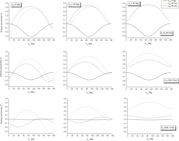
Figure 3: Stokes parameter $P_{1}$ of the Lyman–$\alpha_{1}$ radiation following the radiative recombination of a free electron into the $2p_{3/2}$ state of the bare uranium projectile U⁹²⁺ with energies $T_{p}$ = 10 MeV/u (upper row), 200 Mev/u (middle row) and 600 MeV/u (bottom row). These projectile energies correspond to the kinetic energies of an incoming electron with $E_{0}$ = 5.48 keV, 109.7 keV and 329.1 keV in the ion–rest frame, respectively. The polarization parameter is displayed in the projectile frame and for the axial angles $\phi_{2}\equiv\phi_{Ly}$ = 0^∘ (left column), 45^∘ (middle column) and 90^∘ (right column).

3.4 Polarization correlation studies

Until now, we have discussed the evaluation of the doubly–differential cross section (10) for the two–step radiative recombination. In the following, we shall apply this RR cross section in order to study the angular and polarization correlations between the two emitted photons. We will pay attention especially to two scenarios for these studies. In Section 3.4.1, we shall discuss the polarization of the second, the decay photon as measured in coincidence with the recombination photon whose polarization remains unobserved in this case. In contrast, the angular distribution of the characteristic radiation, following the electron recombination into an excited ionic state and together with the emission of a linearly polarized recombination photon into some particular direction will be obtained later in Section 3.4.2.

3.4.1 Angle–polarization RR studies:

As said above, we shall first analyze the linear polarization of the characteristic radiation by assuming that the polarization properties of the recombination light are not resolved. With this assumption in mind, the differential RR cross section reads as:

$$d\sigma(\hat{n}_{1};\,\hat{n}_{2},\bm{\epsilon}_{2}) = \frac{(2\pi)^{4}}{v_{i}}\frac{2\pi}{\Gamma_{d}}\omega^{2}_{1}\omega^{2}_{2}\,\rho_{00}^{(d)}\,\sum\limits_{\lambda_{1}}\sum_{\mu_{d}\mu^{{}^{\prime}}_{d}\mu_{b}}\sum_{kq}(-1)^{j_{d}-\mu^{\prime}_{d}}C_{j_{d}\mu_{d},\,j_{d}-\mu^{\prime}_{d}}^{kq}A_{kq}^{(d)}$$ (15)

$$\times \left\langle n_{b}j_{b}\mu_{b}\left|R^{+}_{2}\right|n_{d}j_{d}\mu_{d}\right\rangle\left\langle n_{d}j_{d}\mu^{\prime}_{d}\left|R_{2}\right|n_{b}j_{b}\mu_{b}\right\rangle\rm{d}\mathbf{\Omega}_{2}\,.$$

In this expression, we have performed the summation over the spin states of the (first) recombination photons and have fixed its emission angles $\hat{n}_{1}=\left(\theta_{1},\phi_{1}\right)$. Despite this summation, Eq. (15) still contains the complete information about the polarization and angular properties of the subsequent decay radiation which follows the emission of the recombination radiation into a particular direction $\hat{n}_{1}$.

With the help of Eq. (15), we can evaluate the linear polarization of the decay photons. However, before doing so we shall first agree about the parameters which are used in order to characterize both, the degree as well as the direction of such a polarization. From an experimental viewpoint, the polarization of the emitted photons are most easily described in terms of the so–called Stokes parameters which are determined by the intensities of the light $I_{\chi}\sim d\sigma_{\chi}$ linearly polarized under different angles $\chi$ with regard to the reference plane that is spanned by the quantization axis (the beam direction) and the emitted photon momentum $\bm{k}$ (cf. Fig. 1). For instance, while the parameter $P_{1}$

$$P_{1}(\hat{n})=\frac{d\sigma_{0^{\circ}}-d\sigma_{90^{\circ}}}{d\sigma_{0^{\circ}}+d\sigma_{90^{\circ}}}$$ (16)

is derived from the intensities of light, polarized in parallel and perpendicular to the reference plane, the parameter $P_{2}$ follows from a similar ratio, taken at $\chi=45^{\circ}$ and $\chi=135^{\circ}$ respectively:

$$P_{2}(\hat{n})=\frac{d\sigma_{45^{\circ}}-d\sigma_{135^{\circ}}}{d\sigma_{45^{\circ}}+d\sigma_{135^{\circ}}}\,.$$ (17)

As seen from these expressions, any polarization analysis of the characteristic radiation requires the evaluation of the differential cross section describing the emission of linearly polarized (decay) photons under the angles $\hat{n}_{2}=(\theta_{2},\phi_{2})$. Applying the standard decomposition of the linear polarization vector in terms of the circular polarization states [25]:

$$\bm{\epsilon}_{\chi}=\frac{1}{\sqrt{2}}\sum_{\lambda=\pm 1}\exp(-\mathrm{i}\chi\lambda)\bm{\epsilon}_{\lambda},$$ (18)

such a differential cross section can be easily derived from Eq. (15) and from the explicit form of the electron–photon interaction operator $R_{2}$ as:

$$d\sigma(\hat{n}_{1};\,\hat{n}_{2},\bm{\epsilon}_{\chi_{{}_{2}}}) = \frac{(2\pi)^{4}}{v_{i}}\frac{4\pi^{2}\alpha}{\Gamma_{d}}\omega^{2}_{1}\omega^{2}_{2}\,\rho_{00}^{(d)}\,\sum\limits_{\lambda_{1}}\sum\limits_{\lambda_{2}\lambda^{\prime}_{2}}\sum_{\mu_{d}\mu^{{}^{\prime}}_{d}\mu_{b}}\sum_{kq}\exp(\mathrm{i}{\chi}_{2}(\lambda_{2}-\lambda^{\prime}_{2}))(-1)^{j_{d}-\mu^{\prime}_{d}}$$ (19)

$$\times A_{kq}^{(d)}C_{j_{d}\mu_{d},\,j_{d}-\mu^{\prime}_{d}}^{kq}\left\langle n_{b}j_{b}\mu_{b}\left|\bm{\alpha}\cdot\bm{A}^{*}_{\lambda_{2}}\right|n_{d}j_{d}\mu_{d}\right\rangle\left\langle n_{d}j_{d}\mu^{\prime}_{d}\left|\bm{\alpha}\cdot\bm{A}_{\lambda^{\prime}_{2}}\right|n_{b}j_{b}\mu_{b}\right\rangle\rm{d}\mathbf{\Omega}_{2}\,.$$

Together with Eq. (12), this expression enables us to calculate the Stokes parameters (16)–(17) of the subsequent decay photons. Apart from the emission angle $\hat{n}_{2}=(\theta_{2},\phi_{2})$ the polarization Stokes parameters will depend also on the direction $\hat{n}_{1}=(\theta_{1},\phi_{1})$ of the recombination photons, providing thus an opportunity to investigate angle–polarization correlations in the two–step radiative recombination.

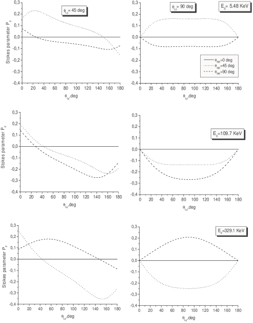
Figure 4: Stokes parameter $P_{2}$ of the Lyman–$\alpha_{1}$ radiation following the radiative recombination of a free electron into the $2p_{3/2}$ state of the bare uranium projectile U⁹²⁺ with energies $T_{p}$ = 10 MeV/u (upper row), 200 Mev/u (middle row) and 600 MeV/u (bottom row). These projectile energies correspond to the kinetic energies of an incoming electron with $E_{0}$ = 5.48 keV, 109.7 keV and, respectively, 329.1 keV in the ion–rest frame. The polarization parameter is displayed in the projectile frame and for the axial angles $\phi_{2}\equiv\phi_{Ly}$ = 45^∘ (left column), and 90^∘ (right column). For the emission of the decay photon within the reaction plane ($\phi_{2}$ = 0^∘), the Stokes parameter $P_{2}$ is zero.

3.4.2 Polarization–angle RR studies:

In our second case, we consider the angular distribution of the characteristic photons with unobserved polarization that follow the emission of (linearly polarized) recombination photons in some given direction $\hat{n}_{1}=(\theta_{1},\phi_{1})$. This angular distribution

$$d\sigma(\hat{n}_{1},\bm{\epsilon}_{\chi_{{}_{1}}};\,\hat{n}_{2}) = \frac{(2\pi)^{4}}{v_{i}}\frac{2\pi}{\Gamma_{d}}\omega^{2}_{1}\omega^{2}_{2}\,\rho_{00}^{(d)}\,\sum\limits_{\lambda_{2}}\sum_{\mu_{d}\mu^{{}^{\prime}}_{d}\mu_{b}}\sum_{kq}(-1)^{j_{d}-\mu^{\prime}_{d}}$$ (20)

$$\times C_{j_{d}\mu_{d},\,j_{d}-\mu^{\prime}_{d}}^{kq}A_{kq}^{(d)}\left\langle n_{b}j_{b}\mu_{b}\left|R^{+}_{2}\right|n_{d}j_{d}\mu_{d}\right\rangle\left\langle n_{d}j_{d}\mu^{\prime}_{d}\left|R_{2}\right|n_{b}j_{b}\mu_{b}\right\rangle\rm{d}\mathbf{\Omega}_{2}\,$$

can be obtained from the general formula (10) upon summation over the spin states of the subsequent photons and by fixing the emission angle and the linear polarization angle $\chi_{1}$ of the recombination light. In Eq. (20), the dependence on the angle and polarization properties of the first (recombination) photon arises from the reduced statistical tensors $A_{kq}^{(d)}=\rho^{(d)}_{kq}/\rho^{(d)}_{00}$ where

$$\rho^{(d)}_{kq}\equiv\rho_{kq}^{(d)}(\theta_{1},\phi_{1},;{\bm{\epsilon}}_{\chi_{{}_{1}}}) = \pi\alpha\sum_{\mu_{d}\mu^{\prime}_{d}\mu_{i}}\,\sum\limits_{\lambda_{1}\lambda^{\prime}_{1}}\,(-1)^{j_{d}-\mu^{\prime}_{d}}\,\exp(\mathrm{i}\chi_{1}(\lambda_{1}-\lambda^{\prime}_{1}))\,C_{j_{d}\mu_{d},\,j_{d}-\mu^{\prime}_{d}}^{kq}$$ (21)

$$\times \left\langle n_{d}j_{d}\mu_{d}\left|\bm{\alpha}\cdot\bm{A}^{*}_{\lambda_{1}}(\theta_{1},\phi_{1})\right|p_{i}\mu_{i}\right\rangle\left\langle p_{i}\mu_{i}\left|\bm{\alpha}\cdot\bm{A}_{\lambda^{\prime}_{1}}(\theta_{1},\phi_{1})\right|n_{d}j_{d}\mu^{\prime}_{d}\right\rangle\,.$$

By evaluating these statistical tensors and by employing them in Eq. (20) we are able to investigate the polarization–angular correlations in the two–step radiative recombination.

4 Results and discussion

In the previous Sections we have derived the general formulas for the differential radiative recombination cross section (10) as well as for the angle–polarization (15) and polarization–angle (20) correlation functions. While these expressions can be applied of course to all hydrogenic states, a more detailed analysis is performed in this work for the electron capture into the $2p_{3/2}$ state of (initially) bare uranium ions U⁹²⁺ and its subsequent Lyman–$\alpha_{1}$ ($2p_{3/2}\to 1s_{1/2}$) radiative decay. The angular and polarization properties of the subsequent characteristic photon emission, as measured in coincidence with the recombination light, will be in the focus of forthcoming experiments at the GSI and FAIR facilities in the next few years.

Let us start our theoretical analysis of the angle and polarization correlations in the two–step RR of bare uranium ions from the computation of the Stokes parameters $P_{1}$ and $P_{2}$ for the Lyman–$\alpha_{1}$ photons. By following an “experimentally realistic” scenario as discussed in Section 3.4.1, we here assume that characteristic photons are measured in coincidence with the recombination radiation whose polarization properties remain however unobserved. For such a scenario, the polarization parameters will depend on both, the nuclear charge $Z$ and the projectile energy $T_{p}$ as well as on the angles under which the recombination and decay photons are observed. In Figures 3 and 4, we display the Stokes parameters $P_{1}$ and $P_{2}$ as functions of the emission angle $\theta_{2}\equiv\theta_{Ly}$ (of the decay photon), and calculated for different angles $\theta_{1}=\theta_{RR}$ = 0^∘, 45^∘ and 90^∘ for the emission of the recombination photon with respect to the beam direction. In addition, we show these (angular) distributions of the polarization parameters also for three observation planes that are tilted by $\phi_{2}$ = 0^∘, 45^∘ and 90^∘ with regard to the reaction plane, and for the three projectile energies $T_{p}$ = 10, 200 and 600 MeV/u, respectively. At these energies, the forward ($\theta_{RR}=0^{\circ}$) emission of the recombination photon results in a parameter $P_{1}$ which is symmetric around $\theta_{Ly}=90^{\circ}$ and does not depend on the axial angle $\phi_{Ly}$, while the Stokes parameter $P_{2}$ vanishes completely. Such a behaviour of polarization parameters is well expected since a recombination photon emission in forward (or backward) direction does not break the axial symmetry for the intermediate “excited ion plus photon” system and, hence, leads to a diagonal density matrix (7) in this case. For this reason, the magnetic sublevel population of the $2p_{3/2}$ excited state can be described by a single non–zero alignment parameter $A_{20}^{(d)}$ (with $A_{2q}^{(d)}=0$ for $q\neq 0$) and this, in turn, results in the symmetric angular distribution of the first Stokes parameter $P_{1}$ and a vanishing second parameter $P_{2}$ (see Ref. [24] for further details).

Of course, the symmetry of the intermediate system is broken in all cases if the recombination photon is observed under an angle $\theta_{RR}\neq 0^{\circ}$ and $\neq 180^{\circ}$. Then, the polarization of the characteristic Lyman–$\alpha$ radiation is described by non–zero parameters $P_{1}$ and $P_{2}$ which are dependent on the axial angle $\phi_{RR}$ and asymmetric with respect to the angle $\theta_{Ly}=90^{\circ}$. Only if the characteristic Lyman–$\alpha_{1}$ photons are measured perpendicular to the reaction plane ($\phi_{Ly}=90^{\circ}$), a symmetric distribution around $\theta_{Ly}=90^{\circ}$ is again restored as can be seen from Eq. (15). For such a perpendicular ($\theta_{Ly}=90^{\circ}$, $\phi_{Ly}=90^{\circ}$) geometry, one may indeed observe a rather strong linear polarization of the Lyman–$\alpha_{1}$ line, especially if the recombination photon is emitted under the angle $\theta_{RR}=45^{\circ}$ with respect to the beam direction. As seen from Fig. 3, for these angles the first Stokes parameter slightly decreases from $P_{1}$ = 0.47 to $0.41$ if the projectile energy is increased from $T_{p}$ = 10 MeV/u to 600 MeV/u.

Until now we analyzed the linear polarization of the characteristic Lyman–$\alpha_{1}$ ($2p_{3/2}\to 1s_{1/2}$) line as measured in coincidence with the recombination photons. In this analysis, we assumed that the spin states of the recombination radiation remain unobserved. In the following, we discuss the “inverse” situation when the (angular) properties of the subsequent decay are observed for the case of a well–defined polarization state of the recombination radiation. Again, we restrict ourselves to the Lyman–$\alpha_{1}$ line whose angular distribution can be obtained from the general expression (20) in the form:

$$\frac{d\sigma(\hat{n}_{1},\bm{\epsilon}_{\chi_{{}_{1}}};\,\hat{n}_{2})}{d\Omega_{2}} = \frac{\sigma_{0}}{4\pi}\,\left(1+\sqrt{\frac{\pi}{5}}\sum\limits_{q}Y_{2q}(\theta_{2},\phi_{2})\,A^{(d)}_{2q}(\hat{n}_{1};{\bm{\epsilon}}_{\chi_{{}_{1}}})\,f_{2}^{3/2,1/2}\right)\,.$$ (22)

Apart from the so–called structure function $f_{2}^{3/2,1/2}$ which describes the mixing between the leading electric–dipole and the (much weaker) magnetic quadrupole decay channels and which takes a value of about $f_{2}^{3/2,1/2}=1.28$ for the hydrogen–like uranium U⁹¹⁺ [15], the angular distribution (22) depends on the five tensor components $A^{(d)}_{2q}(\hat{n}_{1};{\bm{\epsilon}}_{\chi_{{}_{1}}})$, $q=-2,...,2$. As seen from Eqs. (9), (12) and (21) these components are in general complex, and their imaginary and real parts are related to each other as $\mathrm{Re}(A^{(d)}_{21})=-\mathrm{Re}(A^{(d)}_{2-1})$, $\mathrm{Im}(A^{(d)}_{21})=\mathrm{Im}(A^{(d)}_{2-1})$, $\mathrm{Re}(A^{(d)}_{22})=\mathrm{Re}(A^{(d)}_{2-2})$, $\mathrm{Im}(A^{(d)}_{22})=-\mathrm{Im}(A^{(d)}_{2-2})$.

Since the angular distribution (22) of the Lyman–$\alpha_{1}$ radiation is uniquely defined by the components of the reduced statistical tensor $A^{(d)}_{2q}$, we shall first investigate the dependence of these components on the emission angle $\theta_{1}\equiv\theta_{RR}$ and polarization ${\bm{\epsilon}}_{\chi_{{}_{1}}}$ of the recombination photon. Figure 5 displays the real and imaginary parts of the parameters $A^{(d)}_{20}$, $A^{(d)}_{21}$ and $A^{(d)}_{22}$ for the electron capture into the $2p_{3/2}$ state of initially bare uranium ion with projectile energy $T_{p}=1$MeV/u. Calculations are performed in the projectile frame and for the emission of linearly polarized recombination photons with angles $\chi_{1}$ = 0^∘, 45^∘ and 60^∘ with regard to the reaction plane. As expected, the tensor component $A^{(d)}_{20}$ with zero projection $q=0$ is purely real for all these polarization directions. In fact, this component represents the differential (in angle and polarization) alignment parameter and can be expressed in terms of the differential cross sections as:

$$A^{(d)}_{20}(\hat{n}_{1},\bm{\epsilon}_{\chi_{{}_{1}}})=\frac{\frac{d\sigma_{\mu_{d}=+3/2}}{d\Omega_{1}}+\frac{d\sigma_{\mu_{d}=-3/2}}{d\Omega_{1}}-\frac{d\sigma_{\mu_{d}=+1/2}}{d\Omega_{1}}-\frac{d\sigma_{\mu_{d}=-1/2}}{d\Omega_{1}}}{\frac{d\sigma_{\mu_{d}=+3/2}}{d\Omega_{1}}+\frac{d\sigma_{\mu_{d}=-3/2}}{d\Omega_{1}}+\frac{d\sigma_{\mu_{d}=+1/2}}{d\Omega_{1}}+\frac{d\sigma_{\mu_{d}=-1/2}}{d\Omega_{1}}}\,$$ (23)

if the capture of the electron occurs into the magnetic substate $\left|2p_{3/2}\mu_{d}\right\rangle$ and under the simultaneous emission of a photon with polarization vector $\bm{\epsilon}_{\chi_{{}_{1}}}$. As seen from Fig. 5, the differential alignment parameter $A^{(d)}_{20}$ is positive in the forward and backward directions, referring to a preferred population of the two $\mu_{d}=\pm 3/2$ substates. In contrast, the emission of a recombination photon perpendicular to the beam mainly results in the population of the $\mu_{d}=\pm 1/2$ substates which slowly varies from 97.2 % for the polarization angle $\chi_{1}=0^{\circ}$ to 84.0 % for $\chi_{1}=60^{\circ}$.

Beside of the reduced statistical tensor $A^{(d)}_{20}$, which refers to the differential alignment, the spin state of the excited ions in the $2p_{3/2}$ state is also described by the parameters $A^{(d)}_{2\pm 1}$ and $A^{(d)}_{2\pm 2}$, i.e. by the non–diagonal elements of the density matrix. These (additional) parameters also depend on the emission angle as well as the polarization direction $\chi_{1}$ of the recombination photon. While for the polarization angle $\chi_{1}=0^{\circ}$ both parameters $A^{(d)}_{2\pm 1}$ and $A^{(d)}_{2\pm 2}$ are again purely real, they become complex when the linear polarization vector of the recombination photon rotates out of the reaction plane (cf. Fig. 5).

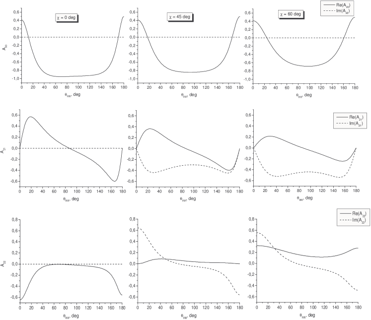
Figure 5: The components $A_{20}$ (upper row), $A_{21}$ (middle row) and $A_{22}$ (bottom row) of the reduced statistical tensor as functions of the recombination photon emission angle $\theta_{1}\equiv\theta_{RR}$. The real (solid line) and imaginary (dashed line) parts of the components are displayed for the capture of an unpolarized electron into the $2p_{3/2}$ state of a bare uranium ion with projectile energy $T_{p}$ = 1 MeV/u, which correspond to the kinetic energy $E=0.55$ keV of the incoming electron in the rest–frame of the ion. Calculations are performed in the projectile frame and for the emission of a recombination photon which is linearly polarized under the angles $\chi=$0^∘ (left column), 45^∘ (middle column) and 60^∘ (right column) with respect to the reaction plane.

Having discussed the properties of the reduced statistical tensors $A^{(d)}_{2q}$, we are now prepared to study the angular distribution (22) of the subsequent Lyman–$\alpha_{1}$ photons. In polarization–angle coincidence measurements, this distribution will depend on both, the polarization state $\bm{\epsilon}_{\chi_{{}_{1}}}$ as well as the angle under which the recombination photon is observed. In Fig. 6 and Fig. 7, for example, we display the angle–differential cross section $d\sigma(\hat{n}_{1},\bm{\epsilon}_{\chi_{{}_{1}}};\,\hat{n}_{2})/d\Omega_{2}$ as calculated for the RR of uranium projectile with energy $T_{p}=$ 1 MeV/u and for the emission of a linearly polarized recombination photon with angles $\chi_{1}=$ 0^∘, 45^∘ and 60^∘, respectively. For these parameters we calculated the differential cross section (22) as a function of the angles $\theta_{1}\equiv\theta_{RR}$ and $\theta_{2}\equiv\theta_{Ly}$ of the recombination and the Lyman–$\alpha_{1}$ photon. Moreover, since the coincidence experiments, as planned at the GSI storage ring, will be carried out most likely in a coplanar geometry (that is, when both photons are detected within the same plane), we have assumed here in the computations that $\phi_{Ly}$ = 0^∘. Again, as expected for this axial angle and for a forward emission of the recombination photon ($\theta_{RR}$ = 0^∘), the Lyman–$\alpha_{1}$ distribution is symmetric around $\theta_{Ly}$ = 90^∘ and also has its minimum at this value since the differential alignment $A^{(d)}_{20}$ is positive in this case (cf. Fig. 5) and the reduced tensor components $A^{(d)}_{2\pm 1}$ vanish identically. For all other angles ($\theta_{RR}\neq$ 0^∘ and $\theta_{RR}\neq$ 180^∘), these statistical tensors are generally non–zero and give rise to an asymmetric distribution of the Lyman–$\alpha_{1}$ photons in coincidence measurements. The asymmetric shift in the angular distribution of the characteristic radiation becomes most pronounced for the emission of the recombination photons under the angle $\theta_{RR}=17^{\circ}$ with respect to the beam direction.

Figure 6: Differential RR cross section (20) as a function of the emission angles of the recombination and the subsequent decay photons. Calculations are performed within the ion–rest frame for the projectile energy $T_{p}$ = 1 MeV/u, axial angle $\phi_{2}\equiv\phi_{Ly}=$ 0^∘ of the decay photon and for the emission of the recombination photon being linearly polarized under the angles $\chi=$0^∘ (left panel), 45^∘ (middle panel) and 60^∘ (right panel) with respect to the reaction plane.

Figure 7: Differential RR cross section (20) as a function of the emission angles of the decay photons. Calculations are performed within the ion–rest frame for the projectile energy $T_{p}$ = 1 MeV/u, axial angle $\phi_{Ly}=0^{\circ}$ (upper row), 45^∘ (middle row) and 90^∘ (lower row) of the decay photon, emission angle $\theta_{RR}=0^{\circ}$ (solid line), 45^∘ (dashed line) and 90^∘ (dotted line) of the recombination photon and for the emission of the recombination photon being linearly polarized under the angles $\chi=$0^∘ (left column), 45^∘ (middle column) and 90^∘ (right column) with respect to the reaction plane.

5 Summary

In this paper, we re–investigated the radiative recombination of a free electron into an excited state of a bare, high–Z ion and its subsequent photon decay. Based on the resonant approximation and the density matrix formalism we derived a general expression for the double–differential RR cross section which accounts for both, the angles and the polarization states of the recombination and the subsequent decay photons. By making use of this differential cross section we studied the polarization and angular correlations between the two emitted photons. In particular, we analyzed how the linear polarization of the characteristic radiation depends on the particular angle under which the recombination photon is observed. In a second scenario, the correlations between the polarization states of the recombination photons and the emission pattern of the subsequent decay have also been discussed. Although the expressions derived in this paper can be applied to any excited hydrogenic state, detailed calculations were performed for the electron capture into the $2p_{3/2}$ state of (initially) bare uranium ions U⁹²⁺ and its subsequent Lyman–$\alpha_{1}$ ($2p_{3/2}\to 1s_{1/2}$) decay. These calculations indicate a rather strong correlation between the polarization states and emission patterns of the recombination and decay photons. Apart from the coplanar geometry, which will be utilized most likely by forthcoming experiments at the GSI storage ring, detailed angular distributions of the Stokes parameters are presented also for a non–coplanar set–up of the detectors. Such a set–up is likely to be implemented at the Super–EBIT facilities. In particular, the geometry of the Stockholm University S–EBIT offers combinations of the observation angles alternative to those available at the GSI storage ring. The angles $\theta_{RR}$ and $\theta_{Ly}$ are limited to 0^∘ or 90^∘ whereas the angle $\phi_{Ly}$ can be varied between 0^∘ and 360^∘ in steps of 45^∘. The non coplanar geometry will be essential for the observation of the linear polarization of the Lyman–$\alpha_{1}$ photons outside of the reaction plane.

6 Acknowledgments

This work was supported by DFG (Grant No. 436RUS113/950/0-1) and by RFBR (Grant No. 08-02-91967). The work of A.V.M. and V.M.S. is also supported by the Ministry of Education and Science of Russian Federation (Program for Development of Scientific Potential of High School, Grant No. 2.1.1/1136). A.S. acknowledges support from the Helmholtz Gemeinschaft (Nachwuchsgruppe VH–NG–421). S.F. is grateful for the support by GSI under the project No. KS–FRT.

References

References

• [1] Stöhlker Th et al 1994 Phys. Rev. Lett. 73 3520
• [2] Stöhlker Th et al 1995 Phys. Rev. A 51 2098
• [3] Stöhlker Th et al 1997 Phys. Rev. Lett. 79 3270
• [4] Stöhlker Th et al 1999 Phys. Rev. Lett. 82 3232
• [5] Eichler J and Meyerhof W 1995 Relativistic Atomic Collisions (San Diego, CA: Academic)
• [6] Shabaev V M, Yerokhin V A, Beier T and Eichler J 2000 Phys. Rev. A 61 052112
• [7] Surzhykov A, Fritzsche S and Stöhlker Th 2001 Phys. Lett. A 289 213
• [8] Shabaev V M 2002 Phys. Rep. 356 119
• [9] Eichler J and Ichihara A 2002 Phys. Rev. A 65 052716
• [10] Klasnikov A E, Artemyev A N, Beier T, Eichler J, Shabaev V M and Yerokhin V A 2002 Phys. Rev. A 66 042711
• [11] Klasnikov A E, Shabaev V M, Artemyev A N, Kovtun A V and Stöhlker Th 2005 NIMB 235 284-289
• [12] Fritzsche S, Indelicato P and Stöhlker Th 2005 J. Phys. B: At. Mol. Phys. B38 S707
• [13] Eichler J, Stöhlker Th 2007 Phys. Rep. 439 1
• [14] Eichler J, Ichihara A and Shirai T 1998 Phys. Rev. A 58 2128
• [15] Surzhykov A, Fritzsche S, Gumberidze A and Stöhlker Th 2002 Phys. Rev. Lett. 88 153001
• [16] Surzhykov A, Fritzsche S and Stöhlker Th 2002 J. Phys. B 35 3713
• [17] Surzhykov A, Fritzsche S and Stöhlker Th 2003 Nucl. Instr. and Meth. in Phys. Res. B 205 391
• [18] Labzowsky L N, Nefiodov A V, Plunien G, Soff G, Marrus R and Liesen D 2001 Phys. Rev. A 63 054105
• [19] GSI conceptual design report 2001
• [20] Stöhlker Th et al 2003 Nucl. Instr. and Meth. in Phys. Res. B 205 210-214
• [21] Tashenov S et al 2006 Phys. Rev. Lett. 97 223202
• [22] Berestetskii V B, Lifshitz V M and Pitaevskii L P 1971 Relativistic Quantum Theory (Oxford: Pergamon)
• [23] Blum K 1981 Density Matrix Theory and Application (New York: Plenum)
• [24] Balashov V V, Grum-Grzhimailo A N and Kabachnik N M 2000 Polarization and Correlation Phenomena in Atomic Collisions (New York: Kluwer Academic)
• [25] Rose M E 1957 Elementary Theory of Angular Momentum (New York: Wiley)
• [26] Grant I 1974 J. Phys. B: At. Mol. Phys. 7 1458
• [27] Surzhykov A, Koval P and Fritzsche S 2005 Comput. Phys. Commun. 165 139