KU-TP 029

Supersymmetric Intersecting Branes
in Time-dependent Backgrounds

Kei-ichi Maeda,^a,b, Nobuyoshi Ohta,^c, Makoto Tanabe^a, and Ryo Wakebe^a,
aDepartment of Physics, Waseda University, Shinjuku, Tokyo 169-8555, Japan

^bWaseda Research Institute for Science and Engineering, Shinjuku, Tokyo 169-8555, Japan
^cDepartment of Physics, Kinki University, Higashi-Osaka, Osaka 577-8502, Japan

We construct a fairy general family of supersymmetric solutions in time- and space-dependent backgrounds in general supergravity theories. One class of the solutions are intersecting brane solutions with factorized form of time- and space-dependent metrics, the second class are brane solutions in pp-wave backgrounds carrying spacetime-dependence, and the final class are the intersecting branes with more nontrivial spacetime-dependence, and their intersection rules are given. Physical properties of these solutions are discussed, and the relation to existing literature is also briefly mentioned. The number of remaining supersymmetries are identified for various configurations including single branes, D1-D5, D2-D6-branes with nontrivial dilaton, and their possible dual theories are briefly discussed.

1 Introduction

The understanding of the fundamental nature and quantum properties of spacetime is one of the most important questions in theoretical physics. An example of such problems is the spacetime singularities that general relativity predicts. A well-known one is the big-bang singularity of a time-dependent spacetime, where general relativity breaks down. One needs a quantum theory of gravity to understand physics close to the singularity. String theory is one of the most promising candidate for such a theory. Although we know some static solutions in string theory, e.g. products of Minkowski space and compact manifolds, these static spacetimes are not so much useful in clarifying the dynamics of string theory in the strong curvature regime or near the singularities. Therefore it is necessary to understand string theory on time-dependent backgrounds. Unfortunately time-dependent backgrounds are difficult to work with in string theories in general, though some special cases are analyzed [1]-[5].

Recently a model of big-bang cosmology has been proposed in matrix string theory based on AdS/CFT correspondence which is a powerful nonperturbative formulation of string theory [6]. This corresponds to a simple time-dependent solution of supergravities which are the low-energy effective theories of string theories that preserves 1/2 supersymmetry in ten dimensions, with the light-like linear dilaton background, and various extensions have been considered [7]-[30]. As is usual in AdS/CFT correspondence, supersymmetry is expected to play an important role. The existence of supersymmetry allows us to better control the behaviors of the solutions in string/supergravity backgrounds and the quantum and nonperturbative properties of the field theories. Therefore there has been much interest in time-dependent supersymmetric solutions of string/supergravity theories. For a detailed review of the big-bang models in string theory, see [31].

On the other hand, D-branes can probe the nonperturbative dynamics of the string theory and they have been used to study various duality aspects of string theory. It is thus interesting to find if we can have such brane solutions in time-dependent backgrounds with time-dependent dilaton. In fact, D3-brane solutions have been found and discussed in [17, 19] and other single brane solutions in [24, 26]. A systematic derivation of the general brane solutions in the pp-wave backgrounds has been given in [32]. It is also interesting to study intersecting brane systems because it is known that some such configurations can describe the standard model of particle physics. More recently, gauge theories on D-branes are examined to gain into the dynamical supersymmetry breaking [33]. These solutions are interesting since the metrics of these solutions depend on both space and time, but the dependence is restricted to the product form of these functions. The question then naturally arises if there are solutions with more general dependence on space and time and if such solutions can give more physical insight.

In this paper, we investigate more general time-dependent supersymmetric solutions in supergravity theories in ten and eleven dimensions in order to understand the nature of spacetime. In sect. 2, we derive brane solutions in general supergravities with dilaton and forms of arbitrary ranks in spacetime-dependent backgrounds. In sect. 3, we give time-dependent solutions restricted to those with time-independent harmonic functions. All known solutions belong to this class of solutions, but our solutions are more general. We clarify the relation of our solutions and the known ones. In sect. 4, we give more general solutions with time-dependent harmonic functions for one brane and two intersecting branes. These are new solutions and the physical properties of these solutions including spacetime and asymptotic structures are discussed in sect. 5. In sect. 6, we show that these solutions have unbroken supersymmetry, and identify the amount of remaining supersymmetries. Sect. 7 is devoted to conclusions and discussions.

2 Time-dependent brane system in supergravity

The low-energy effective action for the supergravity system coupled to dilaton and $n_{A}$- form field strength is given by

$$I=\frac{1}{16\pi G_{D}}\int d^{D}x\sqrt{\mathstrut-g}\left[R-\frac{1}{2}(\partial\Phi)^{2}-\sum_{A=1}^{m}\frac{1}{2n_{A}!}e^{a_{A}\Phi}F_{n_{A}}^{2}\right],$$ (2.1)

where $G_{D}$ is the Newton constant in $D$ dimensions and $g$ is the determinant of the metric. The last term includes both RR and NS-NS field strengths, and $a_{A}=\frac{1}{2}(5-n_{A})$ for RR field strength and $a_{A}=-1$ for NS-NS 3-form. In the eleven-dimensional supergravity, there is a four-form and no dilaton. We put fermions and other background fields to be zero.

From the action (2.1), one can derive the field equations

$$R_{\mu\nu}=\frac{1}{2}\partial_{\mu}\Phi\partial_{\nu}\Phi+\sum_{A}\frac{1}{2n_{A}!}e^{a_{A}\Phi}\Biggl{[}n_{A}\left(F_{n_{A}}^{2}\right)_{\mu\nu}-\frac{n_{A}-1}{D-2}F_{n_{A}}^{2}g_{\mu\nu}\Biggr{]},$$ (2.2)

$$\Box\Phi=\sum_{A}\frac{a_{A}}{2n_{A}!}e^{a_{A}\Phi}F_{n_{A}}^{2},$$ (2.3)

$$\partial_{\mu_{1}}\left(\sqrt{\mathstrut-g}e^{a_{A}\Phi}F^{\mu_{1}\cdots\mu_{n_{A}}}\right)=0\,,$$ (2.4)

where $F_{n_{A}}^{2}$ denotes $F_{\mu_{1}\cdots\mu_{n_{A}}}F^{\mu_{1}\cdots\mu_{n_{A}}}$ and $(F_{n_{A}}^{2})_{\mu\nu}$ denotes $F_{\mu\rho\cdots\sigma}F_{\nu}^{~{}\rho\cdots\sigma}$.

The Bianchi identity for the form field is given by

$$\partial_{[\mu}F_{\mu_{1}\cdots\mu_{n_{A}}]}=0.$$ (2.5)

In this paper we assume the following metric form:

$$ds_{D}^{2}=e^{2\Xi(u,r)}\left[-2dudv+K(u,y^{\alpha},r)du^{2}\right]+\sum_{\alpha=1}^{d-2}e^{2Z_{\alpha}(u,r)}(dy^{\alpha})^{2}+e^{2B(u,r)}\left(dr^{2}+r^{2}d\Omega_{\tilde{d}+1}^{2}\right),$$ (2.6)

where $D=d+\tilde{d}+2$, the coordinates $u$, $v$ and $y^{\alpha},(\alpha=1,\ldots,d-2)$ parameterize the $d$-dimensional worldvolume where the branes belong, and the remaining $\tilde{d}+2$ coordinates $r$ and angles are transverse to the brane worldvolume, $d\Omega_{\tilde{d}+1}^{2}$ is the line element of the $(\tilde{d}+1)$-dimensional sphere. Note that $u$ and $v$ are null coordinates. The metric components $\Xi,Z_{\alpha},B$ and the dilaton $\Phi$ are assumed to be functions of $u$ and $r$, whereas $K$ depends on $u,y^{\alpha}$ and $r$. Our ansatz includes more general solutions than those in [17, 19], which consider only single D3-brane solutions with the metrics of product form of time- and space-dependent factors; ours allows intersecting branes as well as more general spacetime dependence.

For the field strength backgrounds, we take

$$F_{n_{A}}=E_{A}^{\prime}(u,r)\,du\wedge dv\wedge dy^{\alpha_{1}}\wedge\cdots\wedge dy^{\alpha_{q_{A}-1}}\wedge dr,$$ (2.7)

where $n_{A}=q_{A}+2$. Throughout this paper, the dot and prime denote derivatives with respect to $u$ and $r$, respectively. The ansatz (2.7) means that we have an electric background. We could, however, also include magnetic background in the same form as the electric one with the replacement

$$g_{\mu\nu}\to g_{\mu\nu},\quad F_{n}\to e^{a\Phi}*\!F_{n},\quad\Phi\to-\Phi.$$ (2.8)

This is due to the S-duality symmetry of the original system (2.1). So we do not have to consider it separately.

With our ansatz, the Einstein equations (2.2) reduce to

$$\Xi^{\prime\prime}+\Big{(}U^{\prime}+\frac{\tilde{d}+1}{r}\Big{)}\Xi^{\prime}=\sum_{A}\frac{D-q_{A}-3}{2(D-2)}S_{A}(E^{\prime}_{A})^{2},$$ (2.9)

$$\sum_{\alpha=1}^{d-2}\ddot{Z}_{\alpha}+(\tilde{d}+2)\ddot{B}+\sum_{\alpha=1}^{d-2}{\dot{Z}_{\alpha}}^{2}+(\tilde{d}+2){\dot{B}}^{2}-2\dot{\Xi}\left[\sum_{\alpha=1}^{d-2}\dot{Z}_{\alpha}+(\tilde{d}+2)\dot{B}\right]$$

$$+\;\frac{1}{2}\sum_{\alpha=1}^{d-2}e^{2(\Xi-Z_{\alpha})}\partial^{2}_{\alpha}K+e^{2(\Xi-B)}\Bigg{[}K\Xi^{\prime\prime}+\frac{1}{2}K^{\prime\prime}+\Big{(}\Xi^{\prime}K+\frac{1}{2}K^{\prime}\Big{)}\Big{(}U^{\prime}+\frac{\tilde{d}+1}{r}\Big{)}\Bigg{]}$$

$$\hskip 56.9055pt=\sum_{A}\frac{D-q_{A}-3}{2(D-2)}e^{2(\Xi-B)}KS_{A}(E^{\prime}_{A})^{2}-\frac{1}{2}(\dot{\Phi})^{2},$$ (2.10)

$$\dot{\Xi}^{\prime}+\sum_{\alpha=1}^{d-2}\dot{Z}_{\alpha}^{\prime}+(\tilde{d}+1)\dot{B}^{\prime}-\left[\sum_{\alpha=1}^{d-2}\dot{Z}_{\alpha}+(\tilde{d}+2)\dot{B}\right]\Xi^{\prime}-\dot{B}\sum_{\alpha=1}^{d-2}Z_{\alpha}^{\prime}+\sum_{\alpha=1}^{d-2}\dot{Z}_{\alpha}Z_{\alpha}^{\prime}=-\frac{1}{2}\dot{\Phi}\Phi^{\prime},~{}~{}~{}~{}~{}~{}~{}~{}$$ (2.11)

$$Z_{\alpha}^{\prime\prime}+\Big{(}U^{\prime}+\frac{\tilde{d}+1}{r}\Big{)}Z_{\alpha}^{\prime}=\sum_{A}\frac{\delta^{(\alpha)}_{A}}{2(D-2)}S_{A}(E^{\prime}_{A})^{2},$$ (2.12)

$$U^{\prime\prime}+B^{\prime\prime}-\Big{(}2\Xi^{\prime}+\sum_{\alpha=1}^{d-2}Z_{\alpha}^{\prime}-\frac{\tilde{d}+1}{r}\Big{)}B^{\prime}+2(\Xi^{\prime})^{2}+\sum_{\alpha=1}^{d-2}(Z_{\alpha}^{\prime})^{2}$$

$$\hskip 56.9055pt=-\frac{1}{2}(\Phi^{\prime})^{2}+\sum_{A}\frac{D-q_{A}-3}{2(D-2)}S_{A}(E^{\prime}_{A})^{2},~{}~{}~{}~{}~{}$$ (2.13)

$$B^{\prime\prime}+\Big{(}U^{\prime}+\frac{\tilde{d}+1}{r}\Big{)}B^{\prime}+\frac{U^{\prime}}{r}=-\sum_{A}\frac{q_{A}+1}{2(D-2)}S_{A}(E^{\prime}_{A})^{2},$$ (2.14)

where $U$, $S_{A}$ and $\delta_{A}^{(\alpha)}$ are defined by

$$U \equiv 2\Xi+\sum_{\alpha=1}^{d-2}Z_{\alpha}+\tilde{d}B\,,$$ (2.15)

$$S_{A} \equiv \exp\left[\epsilon_{A}a_{A}\Phi-2\left(2\Xi+\sum_{\alpha\in q_{A}}Z_{\alpha}\right)\right],$$ (2.16)

and

$$\delta_{A}^{(\alpha)}=\left\{\begin{array}[]{l}D-q_{A}-3\\ -(q_{A}+1)\end{array}\right.\hskip 14.22636pt{\rm for}\hskip 8.53581pt\left\{\begin{array}[]{l}y^{\alpha}\mbox{ belonging to $q_{A}$-brane}\\ {\rm otherwise}\end{array}\right.,$$ (2.21)

respectively, and $\epsilon_{A}=+1(-1)$ is for electric (magnetic) backgrounds. The sum of $\alpha$ in Eq. (2.16) runs over the $q_{A}$-brane components in the $(d-2)$-dimensional $y^{\alpha}$-space, for example

$$\sum_{\alpha\in q_{A}}Z_{\alpha}=\sum_{\alpha_{A}=1}^{q_{A}-1}Z_{\alpha_{A}}\,.$$ (2.22)

Eqs. (2.9), $\cdots$, (2.13) and (2.14) are the $uv,uu,ur,\alpha\beta,rr$ and $ab$ components of the Einstein equations (2.2), respectively. The dilaton equation (2.3) and the equations for the form field (2.4) and (2.5) yield

$$e^{-U}r^{-(\tilde{d}+1)}(e^{U}r^{\tilde{d}+1}\Phi^{\prime})^{\prime} = -\frac{1}{2}\sum_{A}\epsilon_{A}a_{A}S_{A}(E^{\prime}_{A})^{2},$$ (2.23)

$$\Big{(}r^{\tilde{d}+1}e^{U}S_{A}E_{A}^{\prime}\Big{)}^{\prime} = 0,$$ (2.24)

$$\Big{(}r^{\tilde{d}+1}e^{U}S_{A}E_{A}^{\prime}\Big{)}^{\centerdot} = 0.$$ (2.25)

We assume that $U$ is independent of $r$ but depends only on $u$. In the case of static spacetime, it is known that under this condition ($U$ is constant in case of no dependence on $u$), all the supersymmetric intersecting brane solutions have been derived [34]. If this condition is relaxed, one may get more general non-BPS solutions [35], but here we are interested in the BPS solutions. We extend them to the time-dependent case.

From Eqs. (2.24) and (2.25), we learn that

$$r^{\tilde{d}+1}e^{U}S_{A}E_{A}^{\prime}=c_{A},$$ (2.26)

is a constant. Combined with Eq. (2.23), we then get

$$\Phi^{\prime}=-\frac{1}{2}\sum_{A}\epsilon_{A}a_{A}\frac{c_{A}\tilde{E}_{A}}{r^{\tilde{d}+1}},$$ (2.27)

where we have defined

$$\tilde{E}_{A}=e^{-U}E_{A}.$$ (2.28)

Similarly from Eqs. (2.9), (2.12), (2.14), we find

$$\Xi^{\prime} = \sum_{A}\frac{D-q_{A}-3}{2(D-2)}\frac{c_{A}\tilde{E}_{A}}{r^{\tilde{d}+1}},$$

$$Z_{\alpha}^{\prime} = \sum_{A}\frac{\delta_{A}^{(\alpha)}}{2(D-2)}\frac{c_{A}\tilde{E}_{A}}{r^{\tilde{d}+1}},$$

$$B^{\prime} = -\sum_{A}\frac{q_{A}+1}{2(D-2)}\frac{c_{A}\tilde{E}_{A}}{r^{\tilde{d}+1}}.$$ (2.29)

Note that there is no integral constant in the right hand sides of (2.27) and (2.29). This is related to the BPS condition.

Substituting these into (2.13), we get

$$\sum_{A,B}\Big{[}\frac{c_{A}}{2}M_{AB}+r^{\tilde{d}+1}\left(\frac{1}{\tilde{E}_{A}}\right)^{\prime}\delta_{AB}\Big{]}\frac{c_{B}}{2}\frac{\tilde{E}_{A}\tilde{E}_{B}}{r^{2\tilde{d}+2}}=0,$$ (2.30)

where

$$M_{AB}=\frac{2(D-q_{A}-3)(D-q_{B}-3)}{(D-2)^{2}}+\sum_{\alpha=1}^{d-2}\frac{\delta_{A}^{(\alpha)}\delta_{B}^{(\alpha)}}{(D-2)^{2}}+\tilde{d}\frac{(q_{A}+1)(q_{B}+1)}{(D-2)^{2}}+\frac{1}{2}\epsilon_{A}a_{A}\epsilon_{B}a_{B}.$$ (2.31)

We require that all the branes be independent, and so $E_{A}$ are independent functions. We thus learn from Eq. (2.30) that

$$\frac{c_{A}}{2}M_{AB}+r^{\tilde{d}+1}\left(\frac{1}{\tilde{E}_{A}}\right)^{\prime}\delta_{AB}=0,$$ (2.32)

the off-diagonal part of which is $M_{AB}=0$ for $A\neq B$. As shown in Ref. [34, 27], this condition leads to the intersection rules for two branes. If $q_{A}$-brane and $q_{B}$-brane intersect over ${\bar{q}}\;(\leq q_{A},q_{B})$ dimensions, this gives

$${\bar{q}}=\frac{(q_{A}+1)(q_{B}+1)}{D-2}-1-\frac{1}{2}\epsilon_{A}a_{A}\epsilon_{B}a_{B}.$$ (2.33)

The rule (2.33) tells us that D1-branes with $a_{1}=1$ can intersect with D3-brane with $a_{3}=0$ on a point $(\bar{q}=0)$ and with D5-brane with $\epsilon_{5}a_{5}=-1$ over a string $(\bar{q}=1)$, and D5-brane can intersect with D5-brane over 3-brane $(\bar{q}=3)$, in agreement with Refs. [36, 37, 38].

The second term in (2.32) must be constant. This, in particular, means

$$H_{A}=\sqrt{\frac{2(D-2)}{\Delta_{A}}}\frac{1}{\tilde{E}_{A}}\,,$$ (2.34)

is a harmonic function

$$(r^{\tilde{d}+1}H_{A}^{\prime})^{\prime}=0,\quad(r^{\tilde{d}+1}H_{A}^{\prime})^{{}^{\centerdot}}=0,$$ (2.35)

where we have defined

$$\Delta_{A}=(D-q_{A}-3)(q_{A}+1)+\frac{D-2}{2}a_{A}^{2}.$$ (2.36)

Note, however, that the condition (2.35) allows $u$-dependent term

$$H_{A}=h_{A}(u)+\frac{Q_{A}}{r^{\tilde{d}}},$$ (2.37)

where $h_{A}$ is an arbitrary function of $u$ and $Q_{A}$ is a constant. This class of solutions generalize those discussed in [27]. They are also similar to those discussed in [28] though time-dependence is taken differently.

Using (2.34) in (2.29), we find

$$\Xi = -\sum_{A}\frac{D-q_{A}-3}{\Delta_{A}}\ln H_{A}+\xi(u),$$

$$Z_{\alpha} = -\sum_{A}\frac{\delta_{A}^{(\alpha)}}{\Delta_{A}}\ln H_{A}+\zeta_{\alpha}(u),$$

$$B = \sum_{A}\frac{q_{A}+1}{\Delta_{A}}\ln H_{A}+\beta(u),$$

$$\Phi = \sum_{A}\epsilon_{A}a_{A}\frac{D-2}{\Delta_{A}}\ln H_{A}+\phi(u),$$ (2.38)

where $\xi,\zeta_{\alpha},\beta,\phi$ are functions of $u$ only. It follows from the definition and the solutions (2.38) that $U$ reduces to

$$U=2\xi(u)+\sum_{\alpha=1}^{d-2}\zeta_{\alpha}(u)+\tilde{d}\beta(u),$$ (2.39)

consistent with our ansatz that $U$ depends only on $u$.

The condition (2.24) and (2.25) or (2.26), combined with the definition (2.16) and the solution, gives

$$\epsilon_{A}a_{A}\phi+2\sum_{\alpha\in\kern-2.79996pt/q_{A}}\zeta_{\alpha}+2\tilde{d}\beta=0,$$ (2.40)

$$c_{A}=\tilde{d}Q_{A}\sqrt{\frac{2(D-2)}{\Delta_{A}}}.$$ (2.41)

We then find that $M_{AB}=\frac{\Delta_{A}}{D-2}\delta_{AB}.$ It turns out that using the intersection rules, the condition (2.11) is reduced to

$$(\dot{H}_{A})^{\prime}=0.$$ (2.42)

Namely we find that the harmonic function can be, at most, a sum of the functions of $r$ and $u$. This is consistent with our previous result (2.37) and gives no further constraint.

Note that separable forms for the metric of the type (2.38) was assumed from the beginning in [17, 19, 27, 29], but here we have naturally derived this property. Also the harmonic functions were taken to be independent of $u$, but they can be actually functions of $u$ as well.

We still have to take Eq. (2.10) into our account. This equation is rewritten as

$$W(u,r)+V(u)+\frac{1}{2}\sum_{\alpha=1}^{d-2}e^{2(\Xi-Z_{\alpha})}\partial_{\alpha}^{2}K+\frac{1}{2}e^{2(\Xi-B)}r^{-(\tilde{d}+1)}\left(r^{(\tilde{d}+1)}K^{\prime}\right)^{\prime}=0\,,$$ (2.43)

where

$$W(u,r)\equiv\sum_{A,B}\frac{(D-2)^{2}}{\Delta_{A}\Delta_{B}}(M_{AB}+2)(\ln H_{A})^{\bm{\cdot}}(\ln H_{B})^{\bm{\cdot}}+2\sum_{A}\frac{D-2}{\Delta_{A}}(\ln H_{A})^{\bm{\cdot}\bm{\cdot}}$$

$$\hskip 56.9055pt+\;4(D-2)(\dot{\beta}-\dot{\xi})\sum_{A}\frac{(\ln H_{A})^{\bm{\cdot}}}{\Delta_{A}}\,,$$ (2.44)

$$V(u)\equiv\sum_{\alpha=1}^{d-2}\left(\ddot{\zeta}_{\alpha}+{\dot{\zeta}_{\alpha}}^{2}\right)+(\tilde{d}+2)\left(\ddot{\beta}+{\dot{\beta}}^{2}\right)-2\dot{\xi}\left[\sum_{\alpha=1}^{d-2}\dot{\zeta}_{\alpha}+(\tilde{d}+2)\dot{\beta}\right]+\frac{1}{2}(\dot{\phi})^{2}\,.~{}~{}~{}~{}~{}~{}$$ (2.45)

Eq. (2.43) can be regarded formally as the equation for $K$, which is an elliptic type differential equation with respect to $r$ and $y^{\alpha}$. However the source terms depend not only on $r$ but also on $u$. Hence we have to solve the elliptic type differential equation at any time $u$. It may be very difficult to find the analytic solutions. Instead we may first assume $K$ explicitly, and then solve Eq. (2.43). In this case, Eq. (2.43) must be regarded as a constraint equation for the formally solved variables $\Xi,Z_{\alpha},B$ and $\Phi$. In this paper, we shall adopt the latter approach.

Here we assume

$$K=e^{-2\xi(u)}k(u,y^{\alpha})+{m(u,y^{\alpha})\over r^{\tilde{d}}}\,,$$ (2.46)

with

$$k(u,y^{\alpha}) = k_{0}(u)+\sum_{\alpha=1}^{d-2}k_{\alpha}(u)y^{\alpha}+\sum_{\alpha,\beta=1(\alpha\neq\beta)}^{d-2}k_{\alpha\beta}(u)y^{\alpha}y^{\beta}+\sum_{\alpha\in^{\forall}q_{A}}e^{2\zeta_{\alpha}(u)}h_{\alpha\alpha}(u)(y^{\alpha})^{2},~{}~{}~{}~{}$$ (2.47)

$$m(u,y^{\alpha}) = m_{0}(u)+\sum_{\alpha=1}^{d-2}m_{\alpha}(u)y^{\alpha}\,,$$ (2.48)

where $k_{0}(u),k_{\alpha}(u),k_{\alpha\beta}(u),h_{\alpha\alpha}(u),m_{0}(u)$ and $m_{\alpha}(u)$ are arbitrary functions of $u$. Here the sum $\alpha\in^{\forall}\!\!q_{A}$ is taken only over $y^{\alpha}$ coordinates belonging to all the branes.

Given $K(u,r,y^{\alpha})$, we find that $u$-dependent terms ($\xi,\zeta_{\alpha},\beta$ and $\phi$) are constrained by two conditions (2.40) and (2.43). The solution is then given by

$$ds_{D}^{2} = \prod_{A}H_{A}^{2\frac{q_{A}+1}{\Delta_{A}}}\Bigg{[}e^{2\xi(u)}\prod_{A}H_{A}^{-2\frac{D-2}{\Delta_{A}}}\left(-2dudv+K(u,r,y^{\alpha})du^{2}\right)$$ (2.49)

$$\hskip 56.9055pt+\;\sum_{\alpha=1}^{d-2}\prod_{A}H_{A}^{-2\frac{\gamma_{A}^{(\alpha)}}{\Delta_{A}}}e^{2\zeta_{\alpha}(u)}(dy^{\alpha})^{2}+e^{2\beta(u)}\left(dr^{2}+r^{2}d\Omega_{\tilde{d}+1}^{2}\right)\Bigg{]},$$

$$\tilde{E}_{A}\color[rgb]{0,0,0}=\sqrt{\frac{2(D-2)}{\Delta_{A}}}H^{-1}_{A},\quad\Phi=\sum_{A}\epsilon_{A}a_{A}\frac{D-2}{\Delta_{A}}\ln H_{A}+\phi(u),$$

with two constraints (2.40) and (2.43), where $H_{A}$ and $K$ are given by Eqs. (2.37) and (2.46), respectively, and

$$\gamma_{A}^{(\alpha)}=\left\{\begin{array}[]{l}D-2\\ 0\end{array}\right.\hskip 14.22636pt{\rm for}\hskip 8.53581pt\left\{\begin{array}[]{l}y^{\alpha}\mbox{ belonging to $q_{A}$-brane}\\ {\rm otherwise}\end{array}\right.\,.$$ (2.54)

Note that we still have one gauge freedom for the time coordinate $u$, by which we can choose any function for $\xi(u)$.

To give solutions explicitly, Eqs. (2.40) and (2.43) must still be solved. Let us now discuss explicit solutions.

3 Solutions with time-independent harmonic functions

To see the relation of our results with earlier work, let us first discuss solutions with $u$-independent harmonic functions, i.e.,

$$H_{A}=h_{A}^{(0)}+\frac{Q_{A}}{r^{\tilde{d}}},$$ (3.1)

where $h_{A}^{(0)}$ and $Q_{A}$ are constants. In this case, since $\dot{H}_{A}=0$, we have $W=0$.

We now discuss two examples.

3.1 Branes with factorized metrics in time and space

If $h_{\alpha\alpha}(u)=0(\alpha\in^{\forall}q_{A})$, the conditions on $u$-dependent terms ($\xi,\zeta_{\alpha},\beta$ and $\phi$) should satisfy are Eq. (2.40) and Eq. (2.43) with $W=0$, i.e.

$$\sum_{\alpha=1}^{d-2}\left(\ddot{\zeta}_{\alpha}+{\dot{\zeta}_{\alpha}}^{2}\right)+(\tilde{d}+2)\left(\ddot{\beta}+{\dot{\beta}}^{2}\right)-2\dot{\xi}\left[\sum_{\alpha=1}^{d-2}\dot{\zeta}_{\alpha}+(\tilde{d}+2)\dot{\beta}\right]+\frac{1}{2}(\dot{\phi})^{2}=0\,.~{}~{}~{}~{}~{}~{}$$ (3.2)

The solutions discussed in [19, 29] belong to this class. They consider a single D3-brane with $d=4,\tilde{d}=4$ and take

$$H_{3}=\frac{R^{4}}{r^{4}},~{}~{}e^{2\xi}=e^{2\zeta_{1}}=e^{2\zeta_{2}}\equiv e^{f(u)},~{}~{}K=\beta=0,~{}~{}a_{A}=0,~{}~{}\Phi=\phi(u)\,,$$ (3.3)

where $R$ is a constant. The metrics here are of the factorized form in $u$- and $r$-dependent terms. Eq. (2.40) is trivially satisfied, and Eq. (3.2) gives

$$\ddot{f}-\frac{1}{2}\dot{f}^{2}+\frac{1}{2}\dot{\phi}^{2}=0,$$ (3.4)

in agreement with their result. Here we have more general intersecting solutions with the function $K$.

3.2 Branes in pp-wave backgrounds

Here, we give an example with the pp-wave,

$$K=e^{-2\xi(u)}k(u,y^{\alpha})\,,$$ (3.5)

with (2.47). This is just the case with $m=0$ in Eq. (2.46). The condition (2.43) reduces to

$$V+\sum_{\alpha\in^{\forall}q_{A}}h_{\alpha\alpha}=0,$$ (3.6)

where $V$ is defined by Eq. (2.45). If this condition and Eq. (2.40) are satisfied, the solution is Eq. (2.49) with (3.5).

For a check, let us compare with the D3-brane solution in [17], in which they have $d=4,\tilde{d}=4$ and

$$H=\frac{R^{4}}{r^{4}},~{}~{}e^{2\xi}\equiv k_{\rm CH}^{2}(u)~{},~{}~{}e^{2\xi}K=k(u,y^{\alpha})\equiv h_{\rm CH}(u,r,y^{\alpha}),$$

$$\zeta_{1}=\zeta_{2}=\beta=0,~{}~{}a_{A}=0,~{}~{}\Phi=\phi(u)\equiv\phi_{\rm CH}(u),$$ (3.7)

where $k_{\rm CH},h_{\rm CH},\phi_{\rm CH}$ are the variables adopted in [17]. Again Eq. (2.40) is trivial and Eq. (3.6) reduces to

$$\frac{1}{2}\dot{\phi}^{2}=-h_{11}-h_{22},$$ (3.8)

in agreement with Eq. (12) in [17].

As a more interesting case, let us consider D1-D5-brane solution:

$$ds^{2} = H^{-\frac{3}{4}}_{1}H^{-\frac{1}{4}}_{5}e^{2\xi(u)}\left[-2dudv+K(u,y^{\alpha})du^{2}\right]+\left(\frac{H_{1}}{H_{5}}\right)^{\frac{1}{4}}\sum^{4}_{\alpha=1}e^{\zeta_{\alpha}(u)}dy^{2}_{\alpha}$$

$$+\;H^{\frac{1}{4}}_{1}H^{\frac{3}{4}}_{5}e^{2\beta(u)}\left(dr^{2}+r^{2}d\Omega^{2}_{3}\right),$$

$$\Phi = \ln\left(\frac{H_{1}}{H_{5}}\right)^{\frac{1}{2}}+\phi(u).$$ (3.9)

In this case, $K$ depends on $y^{\alpha}$ linearly because only one spatial dimension in $u$-$v$ coordinates can intersect, and so we take

$$K=e^{-2\xi(u)}\left(k_{0}(u)+\sum_{\alpha=1}^{d-2}k_{\alpha}(u)y^{\alpha}\right).$$ (3.10)

The conditions (2.40) and (3.6) tell us that

$$\phi=4\beta=-\sum_{\alpha=1}^{4}\zeta_{\alpha},~{}~{}\sum_{\alpha=1}^{4}{\dot{\zeta}_{\alpha}}^{2}+12{\dot{\beta}}^{2}=0.$$ (3.11)

The last relation implies that $\zeta_{\alpha}$ and $\beta$ are constant, giving no nontrivial solutions for these. The discussions in [27] overlooked Eqs. (2.11) and (2.25), and so these restrictions on the solution were not obtained.

4 Solutions with time-dependent harmonic functions

In this section, we present more nontrivial solutions with both $r$- and $u$-dependent harmonic functions $H_{A}$ in (2.37). These are the new solutions which have not been known. The metric is also given by (2.49) with (2.37) in the general case. For simplicity of presentation, let us restrict ourselves to the simple case of $K=0$. The nontrivial constraint we still have is the $uu$-component of the Einstein equation (2.43), which reduces to

$$W(u,r)+V(u)=0.$$ (4.1)

As we discussed, we regard this equation as a constraint on the time-dependent part of the harmonic and metric functions. Note that we can easily extend the solution to non-vanishing $K$, if $K$ is given by (2.46). In the case with the quadratic terms of $y^{\alpha}$, the condition (4.1) should be replaced by

$$W(u,r)+V(u)+\sum_{\alpha\in^{\forall}q_{A}}h_{\alpha\alpha}=0.$$ (4.2)

In what follows, we solve Eq. (4.1) and give nontrivial solutions.

4.1 Single brane

We first consider a single $A$-brane. For all branes in M-theory and superstrings, we have the relation

$$\frac{2(D-2)}{\Delta_{A}}=1,$$ (4.3)

so it is sufficient to concentrate on those solutions in which this relation is valid. In this case, (4.1) gives

$$\frac{\ddot{H}_{A}}{H_{A}}+2(\dot{\beta}-\dot{\xi})\frac{\dot{H}_{A}}{H_{A}}+V=0.$$ (4.4)

Substituting (2.37) and sorting out the terms in the orders of $r$, we find

$$\sum_{\alpha=1}^{d-2}\left(\ddot{\zeta}_{\alpha}+{\dot{\zeta}_{\alpha}}^{2}\right)+(\tilde{d}+2)\left(\ddot{\beta}+{\dot{\beta}}^{2}\right)-2\dot{\xi}\left[\sum_{\alpha=1}^{d-2}\dot{\zeta}_{\alpha}+(\tilde{d}+2)\dot{\beta}\right]+\frac{1}{2}(\dot{\phi})^{2}=0,$$ (4.5)

$$\ddot{h}_{A}+2(\dot{\beta}-\dot{\xi})\dot{h}_{A}=0.$$ (4.6)

We can integrate (4.6) to obtain

$$2(\beta-\xi)=-\ln\dot{h}_{A}-2c_{1},$$ (4.7)

where $h_{A}$ is an arbitrary function of $u$, $c_{1}$ is an integration constant and we have additional conditions (2.40) as well as (4.5).

In the present solutions, we have $(d+2)$ arbitrary functions; the metric functions $\xi(u),\zeta_{\alpha}(u),\beta(u)$, the dilaton field $\phi(u)$, and the gauge field $h_{A}(u)$. We still have one constraint (2.40) and two equations (4.5) and (4.7) for those variables. Taking into account one gauge degree of freedom of $u$ coordinate, there are $(d-2)$ degrees of freedom in the present single brane system.

As an example, let us consider D3-brane. In this case, we have six unknown functions of $u$; $\xi,\zeta_{1},\zeta_{2},\beta$, $\phi$, and $h_{3}$, which must satisfy

$$\beta=0,~{}~{}\xi=\frac{1}{2}\ln\dot{h}_{3}+c_{1},~{}~{}\sum_{\alpha=1}^{2}\left(\ddot{\zeta}_{\alpha}+{\dot{\zeta}_{\alpha}}^{2}\right)-\frac{\ddot{h}_{3}}{\dot{h}_{3}}\sum_{\alpha=1}^{2}\dot{\zeta}_{\alpha}+\frac{1}{2}\dot{\phi}^{2}=0.$$ (4.8)

Using the gauge freedom, we may set $\xi=0$. As a result, two functions (e.g. $\zeta_{1}$ and $\zeta_{2}$) remain arbitrary. This gauge choice reduces to $\dot{h}_{3}$=constant, that is $h_{3}=au+b$. If we assume $\zeta_{1}=\zeta_{2}\equiv f(u)/2$ and adopt the gauge condition such that $\xi=f(u)/2$, we find the similar solution in [19, 29], although $h_{3}$ depends on $u$.

4.2 Intersecting two branes

Let us consider two intersecting branes $A$ and $B$. In this case, (4.1) gives

$$\frac{\dot{H}_{A}\dot{H}_{B}}{H_{A}H_{B}}+\frac{\ddot{H}_{A}}{H_{A}}+\frac{\ddot{H}_{B}}{H_{B}}+2\left(\dot{\beta}-\dot{\xi}\right)\left(\frac{\dot{H}_{A}}{H_{A}}+\frac{\dot{H}_{B}}{H_{B}}\right)+V=0.$$ (4.9)

Substituting (2.37) and sorting out the terms in the orders of $r$, we find

$$V=0,$$ (4.10)

$$Q_{B}\ddot{h}_{A}+Q_{A}\ddot{h}_{B}+2\left(\dot{\beta}-\dot{\xi}\right)\left(Q_{B}\dot{h}_{A}+Q_{A}\dot{h}_{B}\right)=0,$$ (4.11)

$$\dot{h}_{A}\dot{h}_{B}+\ddot{h}_{A}h_{B}+h_{A}\ddot{h}_{B}+2\left(\dot{\beta}-\dot{\xi}\right)\left(\dot{h}_{A}h_{B}+h_{A}\dot{h}_{B}\right)=0.$$ (4.12)

To solve the last two equations, we introduce new variables $f_{\pm}(u)$ as

$$h_{A}(u) = \frac{Q_{A}}{2}[f_{+}(u)+f_{-}(u)],$$

$$h_{B}(u) = \frac{Q_{B}}{2}[f_{+}(u)-f_{-}(u)].$$ (4.13)

Eqs. (4.11)and (4.12) are written as

$$\ddot{f}_{+}+2\left(\dot{\beta}-\dot{\xi}\right)\dot{f}_{+}=0,$$ (4.14)

$$(\dot{f}_{+})^{2}=2f_{-}[\ddot{f}_{-}+2(\dot{\beta}-\dot{\xi})\dot{f}_{-}]+(\dot{f}_{-})^{2}.$$ (4.15)

Integrating these equations, we find

$$e^{2(\beta-\xi)}\dot{f}_{+}=c_{+}\,,$$ (4.16)

$$\sqrt{f_{-}(f_{-}-c_{-})}+c_{-}\ln\left[\sqrt{f_{-}}+\sqrt{f_{-}-c_{-}}\right]=f_{+}+c_{0}\,,$$ (4.17)

where $c_{0}$, $c_{\pm}$ are integration constants.

Once we know $\beta(u)$, fixing the gauge (i.e., giving $\xi(u)$), we can solve Eq. (4.16) to obtain $f_{+}(u)$. Then $f_{-}(u)$ is obtained by solving Eq. (4.17). For example, if we choose the gauge as $\xi=\beta$, we find

$$f_{+}(u)=c_{+}u+d_{+}\,,$$ (4.18)

where $d_{+}$ is an integration constant. Then $f_{-}(u)$ is implicitly given by the following equation;

$$\sqrt{f_{-}(f_{-}-c_{-})}+c_{-}\ln\left[\sqrt{f_{-}}+\sqrt{f_{-}-c_{-}}\right]=c_{+}u+d_{+}\,,$$ (4.19)

where we have chosen $c_{0}=0$ without loss of generality.

Compared with the single brane system, our intersecting brane system has one additional function $h_{B}(u)$. On the other hand, there is one additional constraint from (2.40) of the additional brane as well as Eq. (4.10). As a result, naively we expect that $(d-3)$ degree of freedom will be left in the present system. However, there are some exceptional cases. If the number of intersecting dimensions is one, e.g. for D1-D5, D2-D4, and D3-D3 intersecting brane systems, the conditions (2.40) and (4.10) yield that all arbitrary functions vanish, i.e., $\zeta_{\alpha}=\beta=\phi=0$. We can set $\xi=0$ by use of the gauge freedom. As a result no degree of freedom is left in those systems.

We show one concrete example, i.e., the D1-D5-brane system. The solution is given by

$$ds^{2} = -2H^{-\frac{3}{4}}_{1}H^{-\frac{1}{4}}_{5}dudv+\left(\frac{H_{1}}{H_{5}}\right)^{\frac{1}{4}}\sum^{4}_{\alpha=1}dy^{2}_{\alpha}+H^{\frac{1}{4}}_{1}H^{\frac{3}{4}}_{5}\left(dr^{2}+r^{2}d\Omega^{2}_{3}\right),$$

$$\Phi = \ln\left(\frac{H_{1}}{H_{5}}\right)^{\frac{1}{2}}.\,$$ (4.20)

where $H_{A}$ is given by Eq. (2.37) with $A=1$ or 5 and $\tilde{d}=2$. We have chosen $\xi=0$ by using gauge degree of freedom. Then $h_{1}(u)$ and $h_{5}(u)$ are given by Eq. (4.13), i.e,

$$h_{1}(u) = \frac{Q_{1}}{2}[f_{+}(u)+f_{-}(u)],$$

$$h_{5}(u) = \frac{Q_{5}}{2}[f_{+}(u)-f_{-}(u)]\,,$$ (4.21)

where $f_{+}(u)$ is given by Eq. (4.18) and $f_{-}(u)$ is determined by inverting Eq. (4.19) as a function of $u$. Hence the solution is completely fixed up to some integration constants.

Next let us consider D2-D6-brane solution:

$$ds^{2} = H^{-\frac{5}{8}}_{2}H^{-\frac{1}{8}}_{6}\left(-2e^{2\xi(u)}dudv+e^{2\zeta_{1}(u)}(dy^{1})^{2}\right)+H^{\frac{3}{8}}_{2}H^{-\frac{1}{8}}_{6}\sum^{5}_{\alpha=2}e^{2\zeta_{\alpha}(u)}dy^{2}_{\alpha}$$

$$+H^{\frac{3}{8}}_{2}H^{\frac{7}{8}}_{6}e^{2\beta(u)}\left(dr^{2}+r^{2}d\Omega^{2}_{2}\right),$$

$$\Phi = \frac{1}{4}\ln H_{2}-\frac{3}{4}\ln H_{6}+\phi(u)\,.$$ (4.22)

In this case, there are ten non-trivial $u$-dependent functions $\xi,\zeta_{\alpha}(\alpha=1\sim 5),\beta$, $\phi$ and $f_{\pm}$ which must satisfy (2.40), (3.2), (4.16) and (4.17):

$$\sum_{\alpha=2}^{5}\zeta_{\alpha}=-\phi=-\frac{4}{3}\beta\color[rgb]{0,0,0},$$ (4.23)

$$\left(\zeta_{1}+\frac{5}{3}\beta\right)^{\hskip-3.5pt\ddot{~{}}}-2\dot{\xi}\left(\zeta_{1}+\frac{5}{3}\beta\right)^{\hskip-3.5pt\dot{~{}}}+\dot{\zeta}_{1}^{2}+\frac{17}{3}\dot{\beta}^{2}-\sum_{\alpha,\beta=2}^{5}\dot{\zeta}_{\alpha}\dot{\zeta}_{\beta}(1-\delta_{\alpha\beta})=0,~{}~{}~{}~{}~{}~{}~{}~{}~{}$$ (4.24)

$$\beta-\xi=-\frac{1}{2}\left(\ln\dot{f}_{+}-\ln c_{+}\right)\,,$$ (4.25)

$$\sqrt{f_{-}(f_{-}-c_{-})}+c_{-}\ln\left[\sqrt{f_{-}}+\sqrt{f_{-}-c_{-}}\right]=f_{+}+c_{0}\,,$$ (4.26)

where $c_{0},c_{\pm}$ are arbitrary constants. We can set $\xi=0$ by use of the gauge freedom. As a result, we find four arbitrary functions. For example, one can take $\zeta_{2},\zeta_{3},\zeta_{4}$ and $f_{-}$ to be arbitrary functions, and determine $\zeta_{1},\zeta_{5},\beta$, $\phi$ and $f_{+}$ by using the five equations (4.23), (4.24), (4.25) and (4.26).

We can easily extend these solutions to the cases with the $K$-wave if $K$ is given in the form of (2.46).

5 Some Properties of the Solutions

We discuss some properties of our solutions. There are three important geometrical properties of spacetime: a singularity, a horizon, and an asymptotic structure.

5.1 Singularity

To study the spacetime singularity, we have to analyze the curvature tensors. If matter fields are singular at some spacetime region, the Ricci curvature will diverge. For the form and dilaton fields, we have

$$F_{n_{A}}^{2} = -n_{A}!\,e^{-\epsilon_{A}a_{A}\Phi-2B}\left({H_{A}^{\prime}\over H_{A}}\right)^{2}$$ (5.1)

$$= -n_{A}!\,e^{-\epsilon_{A}a_{A}\phi-2\beta}\prod_{B}H_{B}^{-\epsilon_{A}a_{A}\epsilon_{B}a_{B}\frac{D-2}{\Delta_{B}}}\prod_{C}H_{C}^{-2{(q_{C}+1)\over\Delta_{C}}}\left({H_{A}^{\prime}\over H_{A}}\right)^{2},$$

$$e^{\Phi} = e^{\phi(u)}\prod_{A}H_{A}^{\epsilon_{A}a_{A}\frac{D-2}{\Delta_{A}}}.$$ (5.2)

The Ricci scalar is given by

$${\cal R} = \frac{1}{2}(\partial\Phi)^{2}+\frac{1}{2}\sum_{A}\frac{2n_{A}-D}{D-2}e^{-2B}\left({H_{A}^{\prime}\over H_{A}}\right)^{2}\,.$$ (5.3)

Since the harmonic function $H_{A}$ diverges at $r=0$ if the charge $Q_{A}$ does not vanish, we naively expect that matter fields will diverge at $r=0$ as well. However there are some exceptional cases in which matter fields are regular even at $r=0$. We can explicitly show it.

For a single brane system, we find that the second term of the Ricci scalar behaves as

$${\rm the~{}second~{}term~{}of}~{}{\cal R}\propto r^{\frac{2(q_{A}+1)(7-q_{A})}{\Delta_{A}}-2},$$ (5.4)

as $r\rightarrow 0$. It diverges except for $q_{A}=3$ (D3-brane). In the case of the D3-brane, the dilaton coupling vanishes ($a_{A}=0$). The dilaton $\Phi(=\phi(u))$ depends only on $u$ from Eq. (5.2), and then the first term of the Ricci scalar does not diverge either.

We can also calculate the Kretschmann invariant. We find

$${\cal R}_{\mu\nu\rho\sigma}{\cal R}^{\mu\nu\rho\sigma}\propto r^{-\frac{(q_{A}-3)^{2}}{4}}\,,$$ (5.5)

as $r\rightarrow 0$. Hence we again find that D3-brane system is regular even at $r=0$, where branes exist. However other single-brane system has a singularity at $r=0$.

For the D3-brane system, the Kretschmann invariant is given by

$${\cal R}_{\mu\nu\rho\sigma}{\cal R}^{\mu\nu\rho\sigma}=\frac{80Q_{3}^{2}\left(Q_{3}^{2}+12r^{8}h_{3}^{2}\right)}{\left(Q_{3}+r^{4}h_{3}\right)^{5}}\,,$$ (5.6)

where $h_{3}=a_{3}u+b_{3}$ with $a_{3}$ and $b_{3}$ being constants. In that case, $r=0$ is not singular and the curvatures are time independent.

However there appears a singularity at

$$r^{4}=r_{s}^{4}(u)\equiv-{Q_{3}\over a_{3}u+b_{3}}\,.$$ (5.7)

The position of this singularity is time-dependent unless $a_{3}=0$. If $Q_{3}(a_{3}u+b_{3})<0$, i.e. $u<-b_{3}/a_{3}$ (for $a_{3}Q_{3}>0$) or $u>-b_{3}/a_{3}$ (for $a_{3}Q_{3}<0$) the singularity appears at $r_{s}>0$. The Ricci scalar also diverges at the same spacetime position. Hence even if $r=0$ is regular, there appears a singularity in the region of $r>0$ either in the future or on the past. Even if $r_{s}^{4}(u)<0$, because $r=0$ is not singular, we may be able to extend the spacetime beyond $r=0$. Then the singularity appears at $\tilde{r}^{4}\equiv r^{4}+{Q_{3}/(a_{3}u+b_{3})}=0$. The regular brane at $r=0$ is static, but the singularity is moving.

Note that if $a_{3}=0$, setting $b_{3}=1$ and introducing new radial coordinate $\tilde{r}$ by $\tilde{r}^{4}=r^{4}+{Q_{3}}$, we find the metric as

$$ds_{10}^{2} = \left(1-{Q_{3}\over\tilde{r}^{4}}\right)^{1/2}\left[-2dudv+K(u)du^{2}+e^{2\zeta_{1}(u)}(dy^{1})^{2}+e^{2\zeta_{2}(u)}(dy^{2})^{2}\right]$$ (5.8)

$$+ \left(1-{Q_{3}\over\tilde{r}^{4}}\right)^{-2}d\tilde{r}^{2}+\tilde{r}^{2}d\Omega_{5}^{2}\,.$$

This is almost the same as the static D3-brane solution, although there are three time-dependent arbitrary functions, $K,\zeta_{1}$ and $\zeta_{2}$. In this case, not only the regular brane at $\tilde{r}=\sqrt[4]{\mathstrut Q_{3}}$ is static but also the singularity at $\tilde{r}=0$ is time independent.

The analysis of an intersecting two-brane system is similar. The second term in the Ricci scalar is proportional to

$$r^{2\left[7+\bar{q}-(q_{A}+q_{B})\right]\left[\frac{q_{A}+1}{\Delta_{A}}+\frac{q_{B}+1}{\Delta_{B}}\right]-2}\,,$$ (5.9)

in the limit of $r=0$. It diverges except for the cases of $q_{A}+q_{B}=6$ and $\bar{q}=1$, that is, D1-D5, D2-D4 and D3-D3 intersecting-brane systems. In these cases, the dilaton couplings satisfy $a_{A}+a_{B}=0$, hence the dilaton (2.49) is constant near $r=0$. Therefore the Ricci scalar does not diverge. Calculating the Kretschmann invariant in the intersecting two-brane system, we find that $r=0$ is not singular in the D1-D5, D2-D4 and D3-D3 intersecting brane cases, but it is singular for other intersecting two-brane systems. For D1-D5, D2-D4 and D3-D3-brane systems, we find

$${\cal R}_{\mu\nu\rho\sigma}{\cal R}^{\mu\nu\rho\sigma} = \frac{24Q_{1}^{4}Q_{5}^{4}+{\cal O}(r^{2})}{(Q_{1}+r^{2}h_{1})^{9/2}(Q_{5}+r^{2}h_{5})^{11/2}}\,,$$ (5.10)

$${\cal R}_{\mu\nu\rho\sigma}{\cal R}^{\mu\nu\rho\sigma} = \frac{24Q_{2}^{4}Q_{4}^{4}+{\cal O}(r^{2})}{(Q_{2}+r^{2}h_{2})^{19/4}(Q_{4}+r^{2}h_{4})^{21/4}}\,,$$ (5.11)

$${\cal R}_{\mu\nu\rho\sigma}{\cal R}^{\mu\nu\rho\sigma} = \frac{24Q_{3}^{4}Q_{\tilde{3}}^{4}+{\cal O}(r^{2})}{(Q_{3}+r^{2}h_{3})^{5}(Q_{\tilde{3}}+r^{2}{h}_{\tilde{3}})^{5}}\,,$$ (5.12)

respectively. Hence the spacetime structure at $r=0$ is regular, and the spacetime near the branes is static.

The singularities appear at $r^{2}=r^{2}_{s+}(u)$ and $r^{2}=r^{2}_{s-}(u)$, where $r^{2}_{s\pm}$ satisfy

$$r_{s\pm}^{2}(u)\equiv-{2\over f_{+}(u)\pm f_{-}(u)}=-{2\over c_{+}u+d_{+}\pm f_{-}(u)}\,.$$ (5.13)

with $f_{-}(u)$ given by Eq. (4.19).

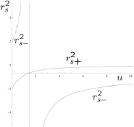
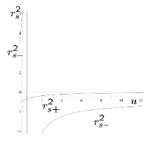
Figure 1: The position ($r_{s}^{2}$) of the singularity with respect to time $u$ for D1-D5-brane system. We set $c_{+}=1,d_{+}=0,c_{-}=1$ (left) and $c_{+}=1,d_{+}=1,c_{-}=1$ (right).

The position of the singularity as $u$ changes is depicted in Fig. 1. If $c_{+}=1,d_{+}=0,c_{-}=1$, $r^{2}_{s+}$ evolves into the $r^{2}>0$ region, which means that the singularity appears beyond the regular position. It can be a naked singularity. On the other hand, if $c_{+}=1,d_{+}=1,c_{-}=1$, $r^{2}_{s+}$ does never go beyond the brane position ($r^{2}=0$). $r^{2}_{s-}$ is also behind $r=0$ for $u>u_{0}(\approx 0.5)$. Hence the singularity is covered by the regular branes.

5.2 Spacetime structure near branes and horizons

As we showed, the systems of single D3-brane, D1-D5, D2-D4 and D3-D3 intersecting two branes are regular at the position of branes ($r=4$). The spacetime structure there is also static.

Assuming $K=0$ and choosing $\xi=0$, if we take the limit of $r=0$ in D3-brane, we find

$$ds_{10}^{2} = Q_{3}^{1/2}\Bigg{[}{1\over z^{2}}\left(-2dudv+dz^{2}\right)+d\Omega_{5}^{2}\Bigg{]}+\;\sum_{\alpha=1}^{2}e^{2\zeta_{\alpha}(u)}(dy^{\alpha})^{2}\,,$$ (5.14)

where $z^{2}=Q_{3}/r^{2}$, and $\xi$ is eliminated by the choice of gauge. We find AdS${}_{3}\times S^{5}\times\tilde{E}^{2}$, where $\tilde{E}^{2}$ is a 2-dimensional time-dependent flat Euclidean space.

In the case of D1-D5, D2-D4, D3-D3 intersecting branes, we find

$$ds_{10}^{2} = Q_{1}^{1/4}Q_{5}^{3/4}\Bigg{[}{1\over z^{2}}\left(-2dudv+dz^{2}\right)+d\Omega_{3}^{2}\Bigg{]}+\;\left({Q_{1}\over Q_{5}}\right)^{1/4}\sum_{\alpha=1}^{4}(dy^{\alpha})^{2},$$

$$ds_{10}^{2} = Q_{2}^{3/8}Q_{4}^{5/8}\Bigg{[}{1\over z^{2}}\left(-2dudv+dz^{2}\right)+d\Omega_{3}^{2}\Bigg{]}+\;\left({Q_{4}\over Q_{2}}\right)^{5/8}(dy^{1})^{2}+\left({Q_{2}\over Q_{4}}\right)^{3/8}\sum_{\alpha=2}^{4}(dy^{\alpha})^{2},$$

$$ds_{10}^{2} = Q_{3}^{1/2}Q_{\tilde{3}}^{1/2}\Bigg{[}{1\over z^{2}}\left(-2dudv+dz^{2}\right)+d\Omega_{3}^{2}\Bigg{]}+\;\left({Q_{\tilde{3}}\over Q_{3}}\right)^{1/2}\sum_{\alpha=1}^{2}(dy^{\alpha})^{2}+\left({Q_{3}\over Q_{\tilde{3}}}\right)^{1/2}\sum_{\alpha=3}^{4}(dy^{\alpha})^{2},$$

where $z^{2}=Q_{A}Q_{B}/r^{2}$. These spacetimes are AdS${}_{3}\times S^{3}\times E^{4}$, where $E^{4}$ is 4-dimensional flat Euclidean space. This is a static spacetime.

As for the horizon, the event horizon can be easily defined if the spacetime is static. However because our spacetime is time dependent, it is not trivial. Rather we may have to look for the apparent horizon. If $K=0$, our spacetime depends only on two variables $u$ and $r$, then one may think that it is easy to find the apparent horizon just as the analysis of the apparent horizon in a spherically symmetric gravitational collapse. However, because $u$ is a null coordinate which is not defined by $r$ but by another spatial coordinate in the brane worldvolume, we have to analyze effectively a three-dimensional problem to find the apparent horizon. One may need numerical analysis, which is beyond the scope of the present study.

In the cases of a single D3-brane, or D1-D5, D2-D4, and D3-D3 intersecting two-brane systems, $r=0$ is not singular but regular and static. Then $r=0$ could be an event horizon in 10 dimensional spacetime. However, we cannot compactify one common brane direction ($y^{d-1}=(v-u)/\sqrt{\mathstrut 2}$), and then we cannot obtain the lower-dimensional black holes

5.3 Asymptotic structure

As for the asymptotic spacetime structure, it is well known if the spacetime is static. In $(\tilde{d}+3)$-dimensional spacetime, we find the asymptotically flat Minkowski geometry, while in the brane directions ($(d-1)$-dimensional space), we have a uniform and static geometry. So compactifying all brane directions, we find an asymptotically flat spacetime.

In the present time-dependent spacetime, we also find a uniform geometry in the brane directions but it is time-dependent. In $(\tilde{d}+3)$-dimensional spacetime, in the limit of $r\rightarrow+\infty$, we find

$$ds_{D}^{2}=-2dudv+\sum_{\alpha=1}^{d-2}f_{\alpha}(u)(dy^{\alpha})^{2}+g(u)d\,{\!\!\!\mbox{ \boldmath$r$}}_{\tilde{d}+2}^{2}\,,$$ (5.16)

where we have used the gauge condition to set $g_{uv}=-1$, i.e.,

$$e^{2\xi}=\prod_{A}h_{A}^{2(D-q_{A}-3)\over\Delta_{A}}\,,$$ (5.17)

and $f_{\alpha}(u)$ and $g(u)$ are given by

$$f_{\alpha}(u)\equiv\prod_{A}h_{A}^{-{2\delta_{A}^{(\alpha)}\over\Delta_{A}}}e^{2\zeta_{\alpha}}\hskip 14.22636pt{\rm and}\hskip 14.22636ptg(u)\equiv\prod_{A}h_{A}^{2(q_{A}+1)\over\Delta_{A}}e^{2\beta}\,\,\,,$$ (5.18)

respectively. If we compactify $y^{\alpha}$, we may find a time-dependent cosmological solution. However, one spatial brane direction ($y^{d-1}$) cannot be compactified, and then such a spacetime is no longer a homogeneous FRW universe. Rather it is just a plane symmetric $(\tilde{d}+3)$-dimensional inhomogeneous spacetime, unless we restrict ourselves to some position in the $y^{d-1}$ direction just as a brane-world scenario.

6 Supersymmetry

In this section, we explore the supersymmetry of our solutions. The supersymmetry transformations in type II supergravities in the Einstein frame are

$$\delta\psi_{\mu}=\Biggl{[}\partial_{\mu}+\frac{1}{4}\omega_{\mu}^{\hat{a}\hat{b}}\Gamma_{\hat{a}\hat{b}}+\frac{1}{8}\sum_{A}e^{\frac{1}{2}\epsilon_{A}a_{A}\Phi}\left(1+\frac{1}{2}\epsilon_{A}a_{A}\right)F/e^{\hat{a}}_{\mu}\Gamma_{\hat{a}}\,\,\Biggr{]}\epsilon\,,$$ (6.1)

$$\delta\lambda=\left[\partial\,/\Phi\,+\sum_{A}\frac{(-1)^{n_{A}}}{2}a_{A}e^{\frac{1}{2}\epsilon_{A}a_{A}\Phi}F/\,\,\right]\epsilon\,,$$ (6.2)

for the dilatino $\lambda$ and the gravitino $\psi_{\mu}$. The supersymmetry parameter $\epsilon$ is a Majorana (complex Weyl) spinor in type IIA (IIB) theory. $\Gamma^{11}$ is given by

$$\Gamma^{11}\equiv\frac{1}{2}\left(\Gamma^{\hat{u}}\Gamma^{\hat{v}}-\Gamma^{\hat{v}}\Gamma^{\hat{u}}\right)\Gamma^{\hat{y}^{1}}\cdots\Gamma^{\hat{y}^{d-2}}\Gamma^{\hat{r}}\Gamma^{\hat{\theta}_{1}}\cdots\Gamma^{\hat{\theta}_{\tilde{d}+1}}\,,$$ (6.3)

and $\Gamma_{\hat{a}\hat{b}}\equiv\Gamma_{[\hat{a}}\Gamma_{\smash{\hat{b}}]}$ are antisymmetrized gamma matrices. The spin connection $\omega_{\mu\hat{a}\hat{b}}$ is defined by

$$\omega_{\mu\hat{a}\hat{b}}\equiv\frac{1}{2}e^{\nu}_{\hat{a}}(\partial_{\mu}e_{\hat{b}\nu}-\partial_{\nu}e_{\hat{b}\mu})-\frac{1}{2}e^{\nu}_{\hat{b}}(\partial_{\mu}e_{\hat{a}\nu}-\partial_{\nu}e_{\hat{a}\mu})-\frac{1}{2}e^{\rho}_{\hat{a}}e^{\sigma}_{\hat{b}}e^{\hat{c}}_{\mu}(\partial_{\rho}e_{\hat{c}\sigma}-\partial_{\sigma}e_{\hat{c}\rho}),$$ (6.4)

where $e_{\mu}^{\hat{a}}$ is a vielbein satisfying $e^{\hat{a}}_{\mu}e_{\hat{a}\nu}=g_{\mu\nu}$ and $e^{\hat{a}}_{\mu}e^{\hat{b}\mu}=\eta^{\hat{a}\hat{b}}$. Note that our Minkowski metric is given by $\eta^{\hat{u}\hat{v}}=\eta^{\hat{v}\hat{u}}=-1,\,\eta^{\hat{u}\hat{u}}=\eta^{\hat{v}\hat{v}}=0$ and $\eta^{\hat{a}\hat{b}}=\delta^{\hat{a}\hat{b}}$ for other indices, because we use double null coordinates. $F/$ denotes the R-R field contracted with gamma matrices; e.g. $F/_{3}=\frac{1}{3!}F_{\mu\nu\rho}\Gamma^{\mu\nu\rho}$. Similarly $\partial\,/\Phi\,=\Gamma^{\mu}\partial_{\mu}\Phi$.

We take $\epsilon$ to be dependent on the coordinates $u$ and $r$ and write $\epsilon=s(u,r)\epsilon_{0}$, where $\epsilon_{0}$ is a constant spinor. The Killing spinor equations are obtained by setting the above transformations (6.1) and (6.2) to zero. We find

$$\delta\psi_{u} = \Biggl{[}\frac{\dot{s}}{s}-\frac{1}{2}\dot{\xi}\left(1+\Gamma_{\hat{u}}\Gamma_{\hat{v}}\right)-\frac{1}{2}e^{\Xi-B}\,\Xi^{\prime}\,\Gamma_{\hat{r}}\Gamma_{\hat{u}}\Biggr{.}$$ (6.5)

$$\qquad+\frac{1}{4}e^{\Xi-B}(K^{\prime}+K\Xi^{\prime})\Gamma_{\hat{r}}\Gamma_{\hat{v}}+\frac{1}{4}\sum_{\alpha=1}^{d-2}e^{\Xi-Z_{\alpha}}\partial_{\alpha}K\Gamma_{\hat{\alpha}}\Gamma_{\hat{v}}$$

$$\qquad\qquad+\;\frac{1}{8}e^{\Xi}\sum_{A}e^{\frac{1}{2}\epsilon_{A}a_{A}\Phi}\left(1+\frac{1}{2}\epsilon_{A}a_{A}\right)F/\left(\Gamma_{\hat{u}}-\frac{1}{2}K\Gamma_{\hat{v}}\right)\Biggr{]}\epsilon_{0}=0,$$

$$\delta\psi_{v} = \Biggl{[}-\frac{1}{2}e^{\Xi-B}\,\Xi^{\prime}\,\Gamma_{\hat{r}}\Gamma_{\hat{v}}+\frac{1}{8}e^{\Xi}\sum_{A}e^{\frac{1}{2}\epsilon_{A}a_{A}\Phi}\left(1+\frac{1}{2}\epsilon_{A}a_{A}\right)F/\Gamma_{\hat{v}}\Biggr{]}\epsilon_{0}=0,$$ (6.6)

$$\delta\psi_{\alpha} = \Biggl{[}\frac{1}{2}e^{Z_{\alpha}-\Xi}\,\dot{Z}_{\alpha}\,\Gamma_{\hat{v}}\Gamma_{\hat{\alpha}}-\frac{1}{2}e^{Z_{\alpha}-B}\,Z_{\alpha}^{\prime}\,\Gamma_{\hat{r}}\Gamma_{\hat{\alpha}}$$ (6.7)

$$\qquad\qquad\qquad\qquad+\;\frac{1}{8}e^{Z_{\alpha}}\sum_{A}e^{\frac{1}{2}\epsilon_{A}a_{A}\Phi}\left(1+\frac{1}{2}\epsilon_{A}a_{A}\right)F/\Gamma_{\hat{\alpha}}\Biggr{]}\epsilon_{0}=0,$$

$$\delta\psi_{r} = \Biggl{[}\frac{s^{\prime}}{s}+\frac{1}{2}e^{B-\Xi}\,\dot{B}\,\Gamma_{\hat{v}}\Gamma_{\hat{r}}+\frac{1}{8}e^{B}\sum_{A}e^{\frac{1}{2}\epsilon_{A}a_{A}\Phi}\left(1+\frac{1}{2}\epsilon_{A}a_{A}\right)F/\Gamma_{\hat{r}}\Biggr{]}\epsilon_{0}=0,$$ (6.8)

$$\delta\psi_{\theta} = \Biggl{[}\frac{1}{2}e^{B-\Xi}\,\dot{B}\,r\,\,\Gamma_{\hat{v}}\Gamma_{\smash{\hat{\theta}}}-\frac{1}{2}(1+r\,B^{\prime})\,\,\Gamma_{\hat{r}}\Gamma_{\smash{\hat{\theta}}}$$ (6.9)

$$\qquad\qquad\qquad\qquad+\frac{1}{8}re^{B}\sum_{A}e^{\frac{1}{2}\epsilon_{A}a_{A}\Phi}\left(1+\frac{1}{2}\epsilon_{A}a_{A}\right)F/\Gamma_{\smash{\hat{\theta}}}\Biggr{]}\epsilon_{0}=0,$$

$$\delta\lambda = \left[\partial\,/\Phi\,+\sum_{A}\frac{(-1)^{n_{A}}}{2}a_{A}e^{\frac{1}{2}\epsilon_{A}a_{A}\Phi}F/\,\,\right]\epsilon_{0}=0.$$ (6.10)

The transformations for other angular components are almost the same as the $\theta$ component and do not give any extra conditions. Now we are going to examine the supersymmetry transformation for several solutions.

6.1 D3-brane system

Let us first consider the time-dependent D3-brane solution in type IIB supergravity, for which the dilaton coupling $a_{A}$ vanishes. Using the self-duality condition, we obtain

$$F/ = \frac{1}{2}\left[F/_{5}+*F/_{5}\right]=\frac{1}{2}\left[F_{uvy^{1}y^{2}r}\Gamma^{uvy^{1}y^{2}r}+\tilde{F}_{\theta_{1}\theta_{2}\theta_{3}\theta_{4}\theta_{5}}\Gamma^{\theta_{1}\theta_{2}\theta_{3}\theta_{4}\theta_{5}}\right]$$ (6.11)

$$= e^{-B}\frac{H_{3}^{\prime}}{H_{3}}\left(\Gamma_{\hat{u}\hat{v}\hat{y}^{1}\hat{y}^{2}\hat{r}}+\Gamma_{\hat{\theta}_{1}\hat{\theta}_{2}\hat{\theta}_{3}\hat{\theta}_{4}\hat{\theta}_{5}}\right),$$

where we have used Eqs. (2.40) and (2.49) to go to the second line. It is easy to see that for the background (2.49), the dilatino variation gives the condition

$$\Gamma_{\hat{v}}\epsilon_{0}=0.$$ (6.12)

The gravitino variation (6.5) takes the form

$$\delta\psi_{u}=\Bigg{[}\frac{\dot{s}}{s}-\frac{1}{2}\dot{\xi}-\frac{1}{16}e^{\Xi-B}\frac{H_{3}^{\prime}}{H_{3}}\Gamma_{\hat{u}\hat{r}}\left(\Bigl{(}1-\Gamma_{\hat{u}\hat{v}\hat{y}^{1}\hat{y}^{2}}\Bigr{)}+\left(1-\Gamma_{\hat{\theta}_{1}\hat{\theta}_{2}\hat{\theta}_{3}\hat{\theta}_{4}\hat{\theta}_{5}\hat{r}}\right)\right)\Bigg{]}\epsilon_{0}=0.$$ (6.13)

The other conditions from (6.6) – (6.10) are similar. One can check that all these conditions are satisfied if $\epsilon$ is given by

$$\epsilon=H_{3}^{-\frac{1}{8}}(u,r)e^{\frac{1}{2}\xi(u)}\epsilon_{0}\,,$$ (6.14)

with

$$\Gamma_{\hat{u}\hat{v}\hat{y}^{1}\hat{y}^{2}}\epsilon_{0}=\epsilon_{0},\quad{\rm and}~{}~{}~{}~{}\Gamma_{\hat{v}}\epsilon_{0}=0\,.$$ (6.15)

Assuming the above conditions are satisfied, we find the last term in Eq. (6.13) automatically vanishes. The condition in (6.14) is needed to kill the $r$- and $u$-dependent terms. The first condition in (6.15) is the standard one for supersymmetry in the presence of a D3-brane and leaves 16 supersymmetries unbroken. We see that the second condition in (6.15) breaks the supersymmetry further by half leaving 8 supersymmetries in total. Namely, compared with the static brane solutions with 16 supersymmetries, it is broken by further one half due to the additional $u$-dependence of the system. All backgrounds of a single brane thus preserve 8 supersymmetries, though we will find that D1-brane is an exceptional case, preserving 16 supersymmetries.

6.2 Intersecting D1-D5-brane system

Next we consider intersecting D1-D5-brane system in type IIB supergravity.

$$F/\,\, = {F/}_{3}+e^{-\Phi}\color[rgb]{0,0,0}*{F/}_{7}=F_{uvr}\Gamma^{uvr}+\tilde{F}_{\theta_{1}\theta_{2}\theta_{3}}\Gamma^{\theta_{1}\theta_{2}\theta_{3}}$$ (6.16)

$$= e^{-B-\frac{1}{2}\Phi}\frac{H_{1}^{\prime}}{H_{1}}\Gamma_{\hat{u}\hat{v}\hat{r}}+e^{-B+\frac{1}{2}\Phi}\frac{H_{5}^{\prime}}{H_{5}}\Gamma_{\hat{\theta}_{1}\hat{\theta}_{2}\hat{\theta}_{3}}.$$

The supersymmetry transformation of dilatino is

$$\delta\lambda = \Biggl{[}-\dot{\Phi}e^{-\Xi}\Gamma_{\hat{v}}+\Phi^{\prime}e^{-B}\Gamma_{\hat{r}}-\frac{1}{2}e^{\frac{1}{2}\Phi}{F/}_{3}\color[rgb]{0,0,0}-\frac{1}{2}e^{-\frac{3}{2}\Phi}*\!{F/}_{7}\color[rgb]{0,0,0}\Biggr{]}\epsilon_{0}$$ (6.17)

$$= \Biggl{[}-\dot{\Phi}e^{-\Xi}\Gamma_{\hat{v}}+\frac{1}{2}e^{-B}\frac{H_{1}^{\prime}}{H_{1}}\Gamma_{\hat{r}}\left(1-\Gamma_{\hat{u}\hat{v}}\right)-\frac{1}{2}e^{-B}\frac{H_{5}^{\prime}}{H_{5}}\Gamma_{\hat{r}}\left(1-\Gamma_{\hat{\theta}_{1}\hat{\theta}_{2}\hat{\theta}_{3}\hat{r}}\right)\Biggr{]}\epsilon_{0}=0.$$

Using $\lambda\;(\Gamma^{11}\lambda=\lambda)$ and $\Gamma^{11}\epsilon=-\epsilon$, we find

$$\Gamma_{\hat{v}}\epsilon_{0}=0,\quad\left(1-\Gamma_{\hat{u}\hat{v}\hat{y}^{1}\hat{y}^{2}\hat{y}^{3}\hat{y}^{4}}\right)\epsilon_{0}=0.$$ (6.18)

We now check the other condition from the gravitino:

$$\delta\psi_{u} =\Biggl{[}\left(\frac{\dot{s}}{s}-\frac{1}{2}\dot{\Xi}\right)-\frac{1}{16}e^{\Xi-B}\Gamma_{\hat{u}\hat{r}}\left(3\frac{H_{1}^{\prime}}{H_{1}}\left(1-\Gamma_{\hat{u}\hat{v}}\right)+\frac{H_{5}^{\prime}}{H_{5}}\left(1-\Gamma_{\hat{\theta}_{1}\hat{\theta}_{2}\hat{\theta}_{3}\hat{r}}\right)\right)\Biggr{]}\epsilon_{0}=0,$$ (6.19)

$$\delta\psi_{r}\color[rgb]{0,0,0} =\Biggl{[}\frac{s^{\prime}}{s}+\frac{3}{16}\frac{H_{1}^{\prime}}{H_{1}}\Gamma_{\hat{u}\hat{v}}+\frac{1}{16}\frac{H_{5}^{\prime}}{H_{5}}\Gamma_{\hat{\theta}_{1}\hat{\theta}_{2}\hat{\theta}_{3}\hat{r}}\Biggr{]}\epsilon_{0}=0.$$ (6.20)

The other conditions are again similar. All these conditions are satisfied if and only if

$$\epsilon=H_{1}^{-\frac{3}{16}}(u,r)H_{5}^{-\frac{1}{16}}(u,r)\,e^{\frac{1}{2}\xi(u)}\,\epsilon_{0}\,,$$ (6.21)

with

$$\Gamma_{\hat{u}\hat{v}\hat{y}^{1}\hat{y}^{2}\hat{y}^{3}\hat{y}^{4}}\epsilon_{0}=\epsilon_{0},\quad\Gamma_{\hat{v}}\epsilon_{0}=0.$$ (6.22)

At first glance, it seems that we have two conditions $\left(1-\Gamma_{\hat{u}\hat{v}}\right)\epsilon=0$ and $\Gamma_{\hat{v}}\epsilon=0$ from (6.17) and (6.19). However it turns out from the property of gamma matrices that these two conditions are equivalent. Thus intersecting D1-D5-brane system also preserves eight supersymmetries. This is a little surprising result because the number of the remaining supersymmetry is the same as the single branes, but this is special for the solutions involving D1-branes.

We also see from this analysis that we get twice the supersymmetries for D1-brane compared with other single branes. The reason is that two conditions coming from the D1-brane and from the time dependence degenerate to one ($\Gamma_{\hat{v}}\epsilon_{0}=0$), but those conditions are independent for the cases of other branes as we have seen in the previous subsection.

6.3 Intersecting D2-D6-brane system

In this final subsection, let us consider the intersecting D2-D6-branes in type IIA supergravity, although it is singular at the branes.

Now we have

$$F/ = {F/}_{4}+e^{-\frac{3}{2}\Phi}\color[rgb]{0,0,0}*{F/}_{8}=F_{uvy^{1}r}\Gamma^{uvy^{1}r}+\tilde{F}_{\theta_{1}\theta_{2}}\Gamma^{\theta_{1}\theta_{2}}$$ (6.23)

$$= e^{-B-\frac{1}{4}\Phi}\frac{H_{2}^{\prime}}{H_{2}}\Gamma_{\hat{u}\hat{v}\hat{y}^{1}\hat{r}}+e^{-B+\frac{3}{4}\Phi}\frac{H_{6}^{\prime}}{H_{6}}\Gamma_{\hat{\theta}_{1}\hat{\theta}_{2}}.$$

The supersymmetry transformation of the dilatino is

$$\delta\lambda = \Biggl{[}-\dot{\Phi}e^{-\Xi}\Gamma_{\hat{v}}+\Phi^{\prime}e^{-B}\Gamma_{\hat{r}}+\frac{1}{4}e^{\frac{1}{4}\Phi}{F/}_{4}\color[rgb]{0,0,0}+\frac{3}{4}e^{-\frac{9}{4}\Phi}*\!F/_{8}\color[rgb]{0,0,0}\Biggr{]}\epsilon_{0}$$ (6.24)

$$= \Biggl{[}-\dot{\Phi}e^{-\Xi}\Gamma_{\hat{v}}+\frac{1}{4}e^{-B}\frac{H_{2}^{\prime}}{H_{2}}\Gamma_{\hat{r}}\left(1-\Gamma_{\hat{u}\hat{v}\hat{y}^{1}}\right)-\frac{3}{4}e^{-B}\frac{H_{6}^{\prime}}{H_{6}}\Gamma_{\hat{r}}\left(1-\Gamma_{\hat{\theta}_{1}\hat{\theta}_{2}\hat{r}}\right)\Biggr{]}\epsilon_{0}=0.$$

So $\epsilon_{0}$ needs to satisfy the conditions

$$\Gamma_{\hat{v}}\epsilon_{0}=0,\qquad(1-\Gamma_{\hat{u}\hat{v}\hat{y}^{1}})\epsilon_{0}=0,\qquad(1-\Gamma_{\hat{u}\hat{v}\hat{y}^{1}\hat{y}^{2}\hat{y}^{3}\hat{y}^{4}\hat{y}^{5}})\epsilon_{0}=0\,.$$ (6.25)

The last term in (6.24) automatically vanishes for given these conditions. The other nontrivial conditions are

$$\delta\psi_{u} = \Biggl{[}\left(\frac{\dot{s}}{s}-\frac{1}{2}\dot{\Xi}\right)-\frac{1}{32}e^{\Xi-B}\Gamma_{\hat{u}\hat{r}}\left(5\frac{H_{2}^{\prime}}{H_{2}}\left(1-\Gamma_{\hat{u}\hat{v}\hat{y}^{1}}\right)+\frac{H_{6}^{\prime}}{H_{6}}\left(1-\Gamma_{\hat{\theta}_{1}\hat{\theta}_{2}\hat{r}}\right)\right)\Biggr{]}\epsilon_{0}=0,$$ (6.26)

$$\delta\psi_{r} = \Biggl{[}\frac{s^{\prime}}{s}+\frac{5}{32}\frac{H_{2}^{\prime}}{H_{2}}\Gamma_{\hat{u}\hat{v}\hat{y}^{1}}+\frac{1}{32}\frac{H_{6}^{\prime}}{H_{6}}\Gamma_{\hat{\theta}_{1}\hat{\theta}_{2}\hat{r}}\Biggr{]}\epsilon_{0}=0.$$ (6.27)

The other components are similar. We find that all these conditions are satisfied if and only if

$$\epsilon=H_{2}^{-\frac{5}{32}}(u,r)H_{6}^{-\frac{1}{32}}(u,r)e^{\frac{1}{2}\xi(u)}\epsilon_{0}\,,$$ (6.28)

with

$$\Gamma_{\hat{u}\hat{v}\hat{y}^{1}}\epsilon_{0}=\epsilon_{0},\quad\Gamma_{\hat{u}\hat{v}\hat{y}^{1}\hat{y}^{2}\hat{y}^{3}\hat{y}^{4}\hat{y}^{5}}\epsilon_{0}=\epsilon_{0},\quad\Gamma_{\hat{v}}\epsilon_{0}=0\,.$$ (6.29)

The first condition in (6.29) comes from the D2-brane, the second one from the D6-brane, the last one from the dilaton. The $r$- and $u$-dependence in (6.28) is needed to kill the $r$- and $u$-dependent terms. Thus intersecting D2-D6-brane system preserves 4 supersymmetries.

7 Concluding Remarks

In this paper we have constructed a fairly general family of time-dependent intersecting brane solutions. An important property of these solutions is that they preserve partial supersymmetry. This is important because this property assures that there will be the corresponding dual field theories according to the gauge/gravity correspondence. The dual theories can be used, for example, to study nonperturbative region of the gravity sector such as the behaviors of the theory close to the singularity.

Our solutions include known D-brane solutions as well as M-branes in time-dependent backgrounds, but the known ones were restricted to those with factorized form of the metrics in time- and space-dependent functions. We have certainly given such solutions but even these are more general. We have also given more general spacetime-dependent solutions with time-dependent harmonic functions where the dependences on time and space cannot be factorized, but they are sum of such terms. These are new class of solutions, and we have studied their singularities, spacetime structure near branes and asymptotic structures.

It is possible that we may get more general solutions if we relax the condition that $U$ depends only on $u$, but it is known that such a generalization gives only non-BPS solutions already for static solutions [35]. So our solutions are expected to be most general BPS solutions with spacetime-dependence.

We have also examined how many supersymmetries remain unbroken in our solutions. The number of those are 8, 8 and 4 for a single brane other than D1, D1-D5-brane and D2-D6-branes, respectively. The 8 remaining supersymmetries on the single brane corresponds to $N=4$ supersymmetry in 2 dimensions and $N=2$ in 4 dimensions. To have remaining supersymmetry, the time dependence can come in only through $u$. Due to this restriction, however, we cannot compactify one worldvolume direction, preventing us from obtaining lower-dimensional black holes, as discussed in sect. 5. It would be thus interesting to study brane solutions with different time dependence, although we would loose unbroken supersymmetry.

The near brane geometry is $AdS_{3}\times S^{5}\times\tilde{E}^{2}$ in the single D3-brane system ($\tilde{E}^{2}$ : two-dimensional time-dependent flat Euclidean space), or $AdS_{3}\times S^{3}\times E^{4}$ ($E^{4}$ : four-dimensional flat Euclidean space) in the D1-D5, D2-D4, and D3-D3-brane systems. As argued in [39], the corresponding dual field theory would be two-dimensional conformal field theory, now in time-dependent backgrounds. It would be interesting to examine the dual field theory [40] and try to understand how the spacetime singularity is described in such a theory. We hope that our construction of these general time-dependent solutions is useful for further study of the singularities and other aspects of the gravitational systems through this kind of dual theories.

Although our solutions include all kinds of brane solutions with RR, NS-NS and eleven-dimensional four-form backgrounds, we have given explicit and detailed discussions of solutions and their properties only for one or two RR fields (D-branes). It is interesting to study our solutions in more detail for the cases including NS-NS field and more branes. It is important because in a static system, we need more than two branes to obtain a black hole solution after compactification to lower dimensions.

Finally though we have constructed the supersymmetric solutions, if we are interested in the direct application (rather than studying singularities and so on) of the solutions to our world, it may be also interesting to consider solutions with dynamical supersymmetry breaking.

References

• [1] H. Liu, G. W. Moore and N. Seiberg, JHEP 0206 (2002) 045 [arXiv:hep-th/0204168]; JHEP 0210 (2002) 031 [arXiv:hep-th/0206182].
• [2] A. Hashimoto and S. Sethi, Phys. Rev. Lett.  89 (2002) 261601 [arXiv:hep-th/0208126].
• [3] J. Simon, JHEP 0210 (2002) 036 [arXiv:hep-th/0208165].
• [4] R. G. Cai, J. X. Lu and N. Ohta, Phys. Lett. B 551 (2003) 178 [arXiv:hep-th/0210206].
• [5] N. Ohta, Phys. Lett. B 559 (2003) 270 [arXiv:hep-th/0302140].
• [6] B. Craps, S. Sethi and E. P. Verlinde, JHEP 0510 (2005) 005 [arXiv:hep-th/0506180].
• [7] M. Li, Phys. Lett. B 626 (2005) 202 [arXiv:hep-th/0506260].
• [8] M. Li and W. Song, JHEP 0510 (2005) 073 [arXiv:hep-th/0507185].
• [9] Y. Hikida, R. R. Nayak and K. L. Panigrahi, JHEP 0509 (2005) 023 [arXiv:hep-th/0508003].
• [10] B. Chen, Phys. Lett. B 632 (2006) 393 [arXiv:hep-th/0508191].
• [11] J. H. She, JHEP 0601 (2006) 002 [arXiv:hep-th/0509067].
• [12] B. Chen, Y. l. He and P. Zhang, Nucl. Phys. B 741 (2006) 269 [arXiv:hep-th/0509113].
• [13] T. Ishino, H. Kodama and N. Ohta, Phys. Lett. B 631 (2005) 68 [arXiv:hep-th/0509173].
• [14] D. Robbins and S. Sethi, JHEP 0602 (2006) 052 [arXiv:hep-th/0509204].
• [15] J. H. She, Phys. Rev. D 74 (2006) 046005 [arXiv:hep-th/0512299].
• [16] B. Craps, A. Rajaraman and S. Sethi, Phys. Rev. D 73 (2006) 106005 [arXiv:hep-th/0601062].
• [17] C. S. Chu and P. M. Ho, JHEP 0604 (2006) 013 [arXiv:hep-th/0602054].
• [18] S. R. Das and J. Michelson, Phys. Rev. D 73 (2006) 126006 [arXiv:hep-th/0602099].
• [19] S. R. Das, J. Michelson, K. Narayan and S. P. Trivedi, Phys. Rev. D 74 (2006) 026002 [arXiv:hep-th/0602107].
• [20] F. L. Lin and W. Y. Wen, JHEP 0605 (2006) 013 [arXiv:hep-th/0602124].
• [21] E. J. Martinec, D. Robbins and S. Sethi, JHEP 0608 (2006) 025 [arXiv:hep-th/0603104].
• [22] H. Z. Chen and B. Chen, Phys. Lett. B 638 (2006) 74 [arXiv:hep-th/0603147].
• [23] T. Ishino and N. Ohta, Phys. Lett. B 638 (2006) 105 [arXiv:hep-th/0603215].
• [24] R. R. Nayak and K. L. Panigrahi, Phys. Lett. B 638 (2006) 362 [arXiv:hep-th/0604172].
• [25] H. Kodama and N. Ohta, Prog. Theor. Phys. 116 (2006) 295 [arXiv:hep-th/0605179].
• [26] R. R. Nayak, K. L. Panigrahi and S. Siwach, Phys. Lett. B 640 (2006) 214 [arXiv:hep-th/0605278].
• [27] N. Ohta and K. L. Panigrahi, Phys. Rev.  D 74 (2006) 126003 [arXiv:hep-th/0610015].
• [28] H. Kodama and K. Uzawa, JHEP 0603 (2006) 053 [arXiv:hep-th/0512104];
P. Binetruy, M. Sasaki and K. Uzawa, arXiv:0712.3615 [hep-th];
K. Maeda, N. Ohta and K. Uzawa, arXiv:0903.5483 [hep-th].
• [29] S. R. Das, J. Michelson, K. Narayan and S. P. Trivedi, Phys. Rev.  D 75 (2007) 026002 [arXiv:hep-th/0610053].
• [30] J. Bedford, C. Papageorgakis, D. Rodriguez-Gomez and J. Ward, arXiv:hep-th/0702093.
• [31] B. Craps, Class. Quant. Grav.  23 (2006) S849 [arXiv:hep-th/0605199].
• [32] N. Ohta, K. L. Panigrahi and S. Siwach, Nucl. Phys. B 674 (2003) 306 [Erratum-ibid. B 748 (2006) 309] [arXiv:hep-th/0306186].
• [33] R. Argurio, M. Bertolini, S. Franco, and S. Kachru, JHEP 0701 (2007) 083 [arXiv:hep-th/0610212]; JHEP 0706 (2007) 017 [arXiv:hep-th/0703236].
• [34] N. Ohta, Phys. Lett. B 403 (1997) 218 [arXiv:hep-th/9702164].
• [35] Y. G. Miao and N. Ohta, Phys. Lett.  B 594 (2004) 218 [arXiv:hep-th/0404082].
• [36] R. Argurio, F. Englert and L. Houart, Phys. Lett.  B 398 (1997) 61 [arXiv:hep-th/9701042].
• [37] G. Papadopoulos and P. K. Townsend, Phys. Lett.  B 380 (1996) 273 [arXiv:hep-th/9603087].
• [38] A. A. Tseytlin, Nucl. Phys.  B 475 (1996) 149 [arXiv:hep-th/9604035].
• [39] J. M. Maldacena and A. Strominger, JHEP 9812 (1998) 005 [arXiv:hep-th/9804085].
• [40] C. S. Chu and P. M. Ho, JHEP 0802 (2008) 058 [arXiv:0710.2640 [hep-th]];
M. R. Gaberdiel and I. Kirsch, JHEP 0704 (2007) 050 [arXiv:hep-th/0703001]