Traveling wave solution of the Reggeon Field Theory

Abstract

We identify the nonlinear evolution equation in impact-parameter space for the “Supercritical Pomeron” in Reggeon Field Theory as a 2-dimensional stochastic Fisher-Kolmogorov-Petrovski-Piscounov equation. It exactly preserves unitarity and leads in its radial form to an high energy traveling wave solution corresponding to an “universal” behaviour of the impact-parameter front profile of the elastic amplitude; Its rapidity dependence and form depend only on one parameter, the noise strength, independently of the initial conditions and of the non-linear terms restoring unitarity. Theoretical predictions are presented for the three typical distinct regimes corresponding to zero, weak and strong noise.

I Introduction

The question of the high-energy behavior of soft hadron-hadron amplitudes and in particular of their expanding impact-parameter disk with rapidity is a rather old subject, but still not solved, being in the basically unknown realm of non-perturbative QCD. However, one promising theoretical approach at early time is the Reggeon Calculus gribov and, in the formalism which we will be dealing with in the present work the Reggeon Field Theory (RFT) abarbanel , where the amplitude is described in terms of an effective quantum field theory of “Pomeron fields”. It derives from a Lagrangean in $2\!+\!1$ dimensions, where “space” is the 2-d impact-parameter $\vec{b}$ and “time”, the overall rapidity $Y.$ In the studie performed during the 70’s, and after a series of works dedicated to the renormalization group approach to the RFT abarbanel , it appeared also supercritical ; ciafaloni ; parisi that a physically interesting case is when one considers instead a “supercritical” bare Pomeron $P$, $i.e.$ when the intercept $\alpha$ is greater than 1 (in fact $\alpha>\alpha_{c}>1,$ where $\alpha_{c}$ includes the quantum effects of the renormalizable RFT when the Pomeron field is at criticality abarbanel ). In that case, unitarity is violated by the bare Pomeron (equivalent to a Born term) but expected to be recovered thanks to damping Pomeron interactions. It was shown that the impact-parameter disk was expanding like the rapidity $Y,$ expressing a dynamical instability ofthe RFT parisi . However, the field theoretical techniques known at that time did not seem to give much more indication on the solutions.

The notion of a Reggeon Field Theory and its use to describe “soft” hadronic interactions appeared, since that time and until recently, under various forms which may differ from the original version depicted in abarbanel . For instance, they may refer to the similar approach deduced or inspired by QCD and its dipole model Iancu ; QCD . Also, there exists a phenomenological interest for using a “supercritical Pomeron” in models based on interacting Pomerons models . So, we want to specify now in which sense we use the RFT and what is different in our approach from the previous ones. First, we want to address the problem of finding the solutions of the full 2-dimensional transverse space problem including an explicit form of the impact-parameter dependence of the elastic amplitude. To our knowledge, explicit solutions have been only found in the zero-dimensional approximation only. Two-dimensional formulations of the QCD Pomeron calculus in the dipole approach are also widely discussed Iancu ; QCD , but explicit solutions seem to be difficult to acquire. So, we restrict our analysis to the initial formulation abarbanel and thus our starting point for the Lagrangean is the original one abarbanel . Hence, when we use the term Reggeon Field Theory (RFT) we refer in the present paper to that precise formulation, up to a suitable generalization to be discussed further on.

The goal of our paper is to update the original study of RFT by introducing new powerful tools known under the name of “traveling wave solutions” of non-linear evolution equations and already used in a different context for QCD evolution equations munier . In fact one of our motivations is to try and give a theoretical answer to an old question raised by the phenomenology of elastic hadronic reactions, and its approach by interacting supercritical Pomerons. The “soft” hadronic elastic amplitudes seem to follow a common behaviour at high-energy, independent of the reaction one considers. While this property could be understood by the factorization properties of a single Regge pole exchange (see, $e.g.$ donach ), it is not known how a property may be obtained from an interacting Pomeron framework where the “bare” Pomeron input is deeply modified by the interactions.

The relation of RFT with non-linear evolution equations (which will allow to use the traveling wave framework) has appeared since long in relation with statistical mechanics of out-of equilibrium processes. Starting with the deep relation between the original RFT with directed percolation critical , there is a long list of works using this kind of connection , in particular with stochastic evolution equation of Langevin type. In fact some of the works (see, $e.g.$ QCD ; Iancu ) are using this connection to try and derive the stochastic evolution equation corresponding to QCD Reggeon Calculus. We shall indeed use some tools from statistical mechanics, in particular those developed in Ref. langevin to transform the RFT formulation in terms of a Langevin equation of known type and possessing traveling wave solutions.

The main feature of traveling wave solutions of non-linear evolution equations is that they lead to “universality” properties, that are properties which will be of general value, $i.e.$ irrespective of particular initial conditions or on features of the equation such as the form of the non-linear damping terms responsible for the unitarity restoration. Our hope is thus to provide through the traveling wave approach, an explicit high-energy solution of the RFT and in the same footing a physical understanding of the empirical “universal” properties of soft scattering amplitudes at high energies which are difficult to explain in a supercritical Pomeron framework. Our paper thus contains the theoretical derivation of the solutions of the (2+1) dimensional RFT abarbanel $via$ the identification of the related stochastic non-linear Langevin equations.

The paper is organized as follows. In section II, we show that the RFT, with a supercritical bare Pomeron as input, can be found equivalently realized by the 2-dimensional version of the stochastic Fisher and Kolmogorov, Piscounov, Petrovsky (sFKPP) equation, and that the elastic amplitude is solution of its reduction to the 1-dimensional radial (azimuthally symmetric) form. In section III, we derive the main feature of the mean field (or deterministic) radial FKPP equation: the existence and universal properties of circular traveling wave asymptotic solutions. In section IV we introduce the effect of stochasticity by analyzing the solution dependence on the noise term. It appears with two markedly different regimes at weak and strong noise strengths. In section VI we present our conclusions and an outlook on the theoretical implications of the traveling wave picture. In the appendices we show the derivation of the solution in the deterministic radial case and an overview on possible phenomenological implications.

II From Reggeon field theory to the 2-d sFKPP equation

The RFT with a supercritical Pomeron is defined abarbanel from the following ingredients, namely one propagator $\cal P\to\cal P,$ with coupling $\mu$ corresponding to the bare supercritical Pomeron intercept $1\!+\!\mu>1.$ There is a kinetic term in impact-parameter space with coupling identified with $\alpha^{\prime},$ the slope of the bare Pomeron trajectory. For the Pomeron interaction vertices, one includes the triple Pomeron vertex, which gives rise to two possible contributions, $i.e.$ the $merging$ triple Reggeon term $\cal P\!+\!\cal P\to\cal P$ and the $splitting$ term $\cal P\to\cal P\!+\!\cal P,$ with initially equal strength $\lambda$ corresponding to the triple-Pomeron coupling.

The field theory action is defined in terms of quantum bosonic fields $\varphi$ and the conjugate $\bar{\varphi}$ by the action abarbanel

$$S[\varphi,\bar{\varphi}]=\frac{1}{\alpha^{\prime}}\ \int\!d^{2}b\ dY\left\{\bar{\varphi}\left[\partial_{Y}\!-\!\alpha^{\prime}\nabla^{2}\right]\varphi\!-\!\mu\ \bar{\varphi}\varphi-i\lambda\left(\bar{\varphi}\varphi^{2}\!+\bar{\varphi}^{2}\varphi\right)\right\}\ .$$ (1)

As discussed in abarbanel , the imaginary coupling constant makes this theory non-hermitian and thus the fields $\varphi$ and $\bar{\varphi}$ do not play a symmetric role through time reversal. It is indeed convenient to perform the field transformation $\varphi\!\to i\varphi,\bar{\varphi}\to-i\bar{\varphi},$ giving rise to the modified action

$$S[\varphi,\bar{\varphi}]=\frac{1}{\alpha^{\prime}}\ \int\!d^{2}b\ dY\left\{\bar{\varphi}\left[\partial_{Y}\!-\!\alpha^{\prime}\nabla^{2}\right]\varphi\!-\!\mu\ \bar{\varphi}\varphi+\lambda\bar{\varphi}\varphi^{2}\!-\lambda\bar{\varphi}^{2}\varphi\right\}\ .$$ (2)

One important outcome of RFT is its remarkable connection with problems of non-equilibrium statistical physics critical . Following a known technique langevin , the fields $\bar{\varphi}$ can be integrated out, and play the role of auxiliary fields appearing as external source fields for the deterministic part (for linear terms in $\bar{\varphi}$) and the noise terms (for quadratic terms in $\bar{\varphi}$) of a non-linear Langevin equation, as we shall now see. Following langevin , one linearizes the remaining quadratic $\bar{\varphi}^{2}$ contribution in (2) by introducing a stochastic white noise via a Stratonovitch transformation, in such a way that all terms become linear in $\bar{\varphi}.$ Then performing the path integral over $\bar{\varphi}$ boils down to a a nonlinear Langevin equation for the field $\varphi$ which now acquires the interpretation of random realizations of the (properly normalized) elastic scattering amplitude $T$, namely

$$\frac{d}{dY}\ T\left(Y,\vec{b}\right)=\alpha^{\prime}\ \nabla^{2}_{b}T+\mu\ T-\lambda\ T^{2}+\sqrt{2\alpha^{\prime}\lambda\ T}\ \nu(Y,\vec{b}\ )\ ,$$ (3)

where the white noise verifies

$$\left\langle{\nu(Y,\vec{b}\ ),\nu(Y^{\prime},\vec{b}^{\prime}\ )}\right\rangle=\delta(Y^{\prime}-Y)\delta^{2}(\vec{b}^{\prime}-\vec{b}\ )\ .$$ (4)

We have now to introduce the appropriate normalization of the scattering amplitude in impact-parameter space which is imposed by the unitarity limit $T\equiv 1.$ This comes as a constraint both on the deterministic and on the stochastic part of (3), since $T\equiv 1$ should appear as a stable fixed point of the equation (the other fixed point is the “unstable” fixed point at $T=0,$ since the rapidity evolution increases, at least in average, the value of $T$). The unitarity constraint thus leads us to modify Eq.(3) to get the following form

$$\frac{d}{dY}\ T\left(Y,\vec{b}\right)=\alpha^{\prime}\ \nabla^{2}_{b}T+\mu\left(T-T^{2}\right)+\sqrt{2\alpha^{\prime}{\bf\kappa}\mu\ (T-T^{2})}\ \nu(Y,\vec{b}\ )\ ,$$ (5)

where it imposes equal coupling $\lambda\equiv\mu$ to the terms in $T$ and $T^{2}$ of the deterministic equation and adding a $T^{2}$ term in the noise factor in order to ensure it to vanish at the black disk limit.

A key feature of Eq.(5) compared to the initial formulation (3) is the introduction of the parameter $\kappa$ which plays a crucial role both physically and mathematically on the nature of the solutions. At first we note that unitarity imposes no a priori constraint on the noise strength and thus allows for the introduction of the parameter $\kappa.$ Physically, $\kappa$ introduces a parametric factor between the strength of the $merging$ term $\cal P\!+\!\cal P\to\cal P$ and the $splitting$ term $\cal P\to\cal P\!+\!\cal P.$ This degree of freedom may come from at least two physial motivations. First, we will see that the traveling wave solutions possess “universal” features, in particular they will remain valid for more complicated $merging$ factors ($e.g.\ T^{n},n>2$ or even with a positive monotonous function $T^{2}f(T)$ with $f(1)=1$). Hence there is $a\ priori$ no constraint of equal coupling between $merging$ and $splitting$ terms. A more intringuing motivation may come from an analogy with the dipole picture. Taking into account their size, the $merging$ and $splitting$ rules for dipoles imply a size-dependence of their effective coupling strength. Indeed, “fat” dipoles may merge more easily than “thin” ones, since it requires a matching of their transverse coordinates, while splitting does not seem to require such an effect. All in all, we find it physically suitable to consider the generalized Eq.(5) as the basic equation to be solved. Obviously taking $\kappa=1,$ we recover the original RFT, up to a quadratic $T^{2}$ term in the noise which is easy to reinterpret as a four-vertex, see further.

Our basic starting point is to point out that Eq.(5) is (by introducing canonical variables, see further) the extension in two spatial dimensions of the Fisher and Kolmogorov, Piscounov, Petrovsky (FKPP) equations (for $\kappa=0$), or (for $\kappa\neq 0$) its stochastic extension (sFKPP), see Refs.FKPP ; wave ; brunet ; wave1 ; mueller ; munier . This will allow us to find the solutions of the RFT for a supercritical bare Pomeron, thanks to modern tools applied to the old and yet unsolved RFT problem.

Mathematically speaking, we are looking for solutions which are not dependent of the forms of the non-linear terms provide they ensure a stable fixed point, that is $T=1$ in our case. $Universality$ also means that the solution is independent of the initial conditions after some “time” (here, rapidity) evolution interval. This defines a “universality class” of solutions, which will ultimately depend only of the value of $\kappa,$ that is on the noise strength. If we were in the situation of statistical physics at equilibrium , we could consider $\kappa$ as the order parameter of the problem. In our case it will allow to separate different regimes (but not necessarily separated by critical points.) We also note that the quadratic term in the noise can be easily reinterpreted in the field theoretical framework as a $\cal P\!+\!\cal P\to\cal P\!+\!\cal P$ coupling in the RFT framework. This is equivalent to the following RFT action

$$S[\varphi,\bar{\varphi}]=\frac{1}{\alpha^{\prime}}\ \int\!d^{2}b\ dY\left\{\bar{\varphi}\left[\partial_{Y}\!-\!\alpha^{\prime}\nabla^{2}\right]\varphi\!-\!\mu\ \bar{\varphi}(\varphi\!-\varphi^{2})\!-\!\kappa\mu\ \bar{\varphi}^{2}(\varphi-\varphi^{2})\right\}\ .$$ (6)

To complete the theoretical preliminaries it is worth mentioning that from the point of view of statistical physics, it is known that more general Langevin equations can in turn be analyzed in terms of a bosonic quantum field theory cyrano . This formalism is particularly convenient to treat fluctuations superimposed to mean-field equations. Hence both techniques coming from statistical and particle physics can be joined together to get a deeper understanding of the original RFT problem and find the structure of its solutions, $i.e.$ identifying its “universality class”.

Let us introduce now canonical variables allowing to put (5) in the generic form of the sFKPP equation. By suitable redefinitions

$$T(Y,\vec{b})\equiv\ U(t,\vec{r})\quad;\quad\mu(Y\!-Y_{0})=t\quad;\quad\sqrt{\frac{\mu}{\alpha^{\prime}}}\ \vec{b}=\vec{r}\quad;\quad\ \epsilon=\ \sqrt{2\mu\kappa}\ ,$$ (7)

Eq. (5) can be recast in the canonical form

$$\frac{d}{dt}\ U\left(t,\vec{r}\right)=\nabla^{2}_{r}U+\ U-\ U^{2}+\epsilon\ \sqrt{U(1-U)}\ \nu(t,\vec{r})\ ,$$ (8)

where the only remaining dimensionless parameter defines the normalized noise strength $\epsilon$ as a function of the product of the “splitting over merging” factor $\kappa,$ and the “super-criticality parameter” $\mu.$ Eq. (8) is the canonical form of the nonlinear stochastic Fisher-Kolmogorov-Petrovski-Piscounov (FKPP) equation. It is worthwhile to note that the time relation in (7) is defined up to a rapidity translation $Y\!-Y_{0}.$

To remind known properties in dimension one, the remarkable feature of the FKPP class of equations FKPP ; wave ; wave1 ; munier is to admit asymptotic traveling wave solutions, $i.e.$ solutions which depend neither on the initial conditions nor on the precise form of the nonlinear term at large enough evolution time. In the example of the deterministic case (without noise), we display a sketch of the traveling wave solutions of the 1d FKPP equation on Fig.1.

Figure 1: Traveling waves in 1 dimension. The traveling waves are asymptotic solutions $u(x,t)$ of the 1-dimensional FKPP equation, translation invariant in time and joining the unstable fixed point (transparency i.e. dilute medium), to the stable fixed point (strong absorption i.e. dense medium). The figure is from Ref.munier .

For sFKPP, the stochastic form of the 1-d equation, following a series of applications to QCD munier ; Iancu , the recently found solutions mumu can be interpreted as a stochastic superposition of traveling waves (see also beuf ).

Our aim is to look for similar properties for the 2-d version of the FKPP equation and find their consequences for the high-energy elastic amplitude, solution of the RFT. Our main results is the prediction of an asymptotic “universal” scaling form of the soft elastic amplitude $T(Y,\vec{b})$ and in particular the prediction of an asymptotic expression for the expanding impact-paramter disk.

The study of the general 2-d sFKPP equation (8) is interesting in itself and some results have been obtained already in the statistical physics literature ($e.g.$ studies on the instabilities of the front wave kessler ). In the following, due to the rotational symmetry in impact-parameter space of the elastic amplitude we shall concentrate our analysis of Eq.(5) to radial amplitudes, $i.e.$ depending spatially only on the radial coordinate $r=|\vec{r}|.$ A comment is in order at this stage. Indeed, one could consider non azimuthally symmetric fluctuations contributing to a symmetric average. However, both the stochastic and the nonlinear character of the equation seems to invalidate this possibility. In particular anisotropic evolution may be caused by the noise kessler and thus lead to a forbidden azimuthal symmetry breaking of the solution . We will assume that, if physical azimuthally assymetric fluctuations of the amplitude may exist, they are azimuthally averaged after a characteristic time much smaller than the typical evolution time in rapidity.

One then obtain, after obvious integration over the azimuth, the following equation to be studied

$$\frac{d}{dt}\ U\left(t,r\right)=\partial_{rr}\ U+\frac{1}{r}{\partial_{r}}\ U+\ U-\ U^{2}+\epsilon\ \sqrt{\frac{U(1-U)}{2\pi r}}\ \ \nu(t,r)\ ,$$ (9)

where a curvature term $\frac{1}{r}\partial_{r}U$ appears in addition to the original 1-dimensional FKPP equation (5). Note also the modification of the noise strength by a factor $1/{2\pi r}$ reflecting the symmetry constraint on the fluctuation strength. The white noise satisfies $\left\langle{\nu(t,r),\nu(t^{\prime},r^{\prime})}\right\rangle=\delta(t^{\prime}\!-\!t)\delta(r^{\prime}\!-\!r)$. Looking for the asymptotic universal solutions of Eq.(9) in terms of circular circular traveling waves in impact-parameter space is the goal of our paper.

III Circular traveling waves: Deterministic case

Let us first consider the equation (9) without the noise term, $i.e.\ \epsilon=0,$ namely the radial extension of the 2-d deterministic FKPP equation. It corresponds to neglecting the Pomeron loop contributions in the high-energy elastic amplitude. A series of results have been obtained for the 1-dimensional FKPP equation. The same methods, which we will adapt for the radial case, lead to new results. Indeed, the radial case is adding the derivative term $\frac{1}{r}\partial_{r}U$ to the standard FKPP equation and work in the half line $r\in[0,\infty]$. The deterministic equation to be studied is thus

$$\frac{d}{dt}\ U\left(t,r\right)=\partial_{rr}\ U+\frac{1}{r}\ \partial_{r}\ U+\ U-\ U^{2}\ .$$ (10)

We will prove the existence of traveling wave asymptotic solutions, which appear now as circular traveling waves (picturally reminiscent of those created by a stone falling in water).

Let us recall first the main guiding principles of the FKPP traveling wave analysis. One distinguishes wave1 different regions, starting from the forward towards the backward of the wave, namely: the “very forward” region, the “leading edge”, the “wave interior” and the “saturation” regions. The universality properties mainly pertain to the “leading edge” region and its transition to the “wave interior”. In order to fulfill these universality conditions, characterizing the “critical” regime whence the traveling waves are formed, the initial conditions should be sharp enough in impact parameter, $i.e.$ $U(t=t_{0},r\gg r_{0})<e^{-r}$. This condition is fulfilled by considering an initial Gaussian form $e^{-r^{2}/4B}$ in impact-parameter. We will keep this point-of-view in the following by considering $e.g.$ a supercritical bare pomeron equipped with a Gaussian form in impact-parameter.

Indeed, in the critical regime of high rapidity, the “very forward” region is driven by the initial condition, while the “leading edge” one develops a “universal” behavior wave1 where three terms of the asymptotic expansion of the amplitude do not depend either on the details of the initial condition or on the nonlinear damping term. The “wave interior” posseses an exact scaling property (see further) while the “saturation” region depends on the nonlinear term. So, for completion, we will also give some hint on this region in the particular case of the initial RFT $(\kappa=1)$ with a triple Pomeron coupling.

In fact the main universal property of the traveling wave solutions in the deterministic case is the scaling property, namely

$$U(t,r)\ \equiv\ U(r-r_{s}(t))\ ,$$ (11)

where the “time” dependent radius $r_{s}(t)$ plays the role of the “saturation scale” in QCD munier .

III.1 Universal “Leading edge” region

Let us now derive the traveling wave properties in the radial case. For the leading edge, following a similar procedure for the 1-dimensional problem brunet ; beuf , one introduces in (10) an ansatz

$$U\left(t,s=r\!-\!v_{c}t\right)\ \propto\ \exp{\left[-\gamma_{c}(s+c(t))\right]}\ t^{\alpha}\ G\left(\frac{s+c(t)}{t^{\alpha}}\right),$$ (12)

where $v_{c}$ ($resp.\ \gamma_{c}$) is the critical wave velocity ($resp.$ critical slope) of the traveling wave front and $c(t)$ describes the sub-asymptotic correction to the velocity $v(t)\equiv v_{c}+\partial c(t)/\partial t$. This ansatz describes the “velocity blocking” due to the critical mechanism. The point is that, being situated in the forward region where the non-linear terms in (10) may be neglected, the form of the ansatz can be deduced from the linear part of the deterministic equation (10). The only effect of the non-linearity is to ensure the “velocity blocking” by the compromise between the fast moving very-forward regime and the damping due to the non-linear unitarity bound (see, $e.g.$ munier ).

Inserting the ansatz in the equation (10) and neglecting the small contribution from the nonlinear term to the leading edge, we can verify the equation for the dominant terms (successively in $t^{0},t^{-1/2},t^{-1}$) of the time expansion, see Appendix A. Note that the condition $G(z)\to z$ when $z\to 0,$ is required in order to match with the scaling region (called the “wave interior” in wave1 ).

Adapting to the radial case the standard procedure brunet ; beuf , one finds

$$U(r\!-\!r_{s},t) \sim \ (r\!-\!r_{s})\ \exp{\left\{-\ (r\!-\!r_{s})-\ \frac{(r-r_{s})^{2}}{\!4\ t}\right\}}\ ,$$

$$r_{s} = v_{c}t+c(t)=2t-{\bf 2}\log t\ ,$$ (13)

where $r_{s}$ is the average time position of the wave front (or “saturation scale” in the language of QCD munier ). Note that the form of the leading-edge front is the same as the one obtained in the 1-dimensional problem brunet ; munier while the saturation scale is $r_{s}=2t-{\bf 2}\log t$ instead of $r_{s}=2t-{\bf\frac{3}{2}}\log t,$ due to the contribution of the new term $\frac{1}{r}\partial_{r}U$ characteristic of the 2-dimensionality of the initial physical picture. The saturation scale evolution is thus slower by a logarithmic factor ${\bf\frac{1}{2}}\log t.$ This $\bf 1/2$ shift is due to the purely geometrical “curvature contribution” of the 2-dimensional problem derrida which combines with the coefficient $\bf 3/2$ of the FKPP solutions. A third (and last) universal term in $r_{s}$ behaving as $t^{-1/2}$ can also be derived and will add some new curvature contributions.

The scaling (11) is recovered from (13) in the region $\frac{(r-r_{s})^{2}}{\!4\ t}\ll 1$ giving rise to the simple expression

$$U(r\!-\!r_{s})\sim\ (r\!-\!r_{s})\ \exp{\left[-(r\!-\!r_{s})\right]}\ ,$$ (14)

where it ensures the transition with the “wave interior” domain.

III.2 Circular wave properties for a triple Pomeron coupling

III.2.1 Deep “Wave interior” region

Taking into account now the specific quadratic nonlinear term of (10) (reflecting the original triple Pomeron coupling), we can explore the deep “wave interior” regime, adapting a method logan used for the similar problem in the QCD case parametric .

Considering a scaling ansatz with an expansion in a small parameter $\Delta^{-2}$ to be determined by consistency with the scaling form (14),

$$U\equiv U\left(z\equiv\frac{r-\int^{t}dt^{\prime}v(t^{\prime})}{\Delta}\right)=U_{0}+\Delta^{-2}\ U_{2}+\Delta^{-4}\ U_{4}+\cdots\ ,$$ (15)

one obtains (see appendix B)

$$U=\frac{1}{1+e^{z}}+\Delta^{-2}\ \frac{e^{z}}{\left(1+e^{z}\right)^{2}}\ \log{\frac{\left(1+e^{z}\right)^{2}}{4e^{z}}}+{\cal{O}}(\Delta^{-4})\ .$$ (16)

with

$$z\equiv\frac{r-\int^{t}dt^{\prime}v(t^{\prime})}{\Delta}\Leftrightarrow\frac{r-r_{s}}{2}\ ,$$ (17)

where the equality isobtained by matching at high enough $t$ with the critical velocity of the leading-edge solution, namely $\Delta=2.$ Note that it is easy to determine higher order terms by a system of nested linear differential equations.

III.2.2 “Saturation” region

The circular traveling waves being concentric around $r=0,$ the saturation region at small $r$ is naturally expected to be different from the 1-dimensional one depicted in Fig1, where saturation starts from $-\infty.$ This is also made explicit by the $\partial_{r}U/r$ term in Eq.10, which can no more be neglected or considered as giving second order effects as in the previous regions. For describing the saturation region, it is useful to go back to the full 2-dimensional form (8). It is convenient to introduce the S-Matrix element $S=1-T,$ which is expected to be small in the saturation region. In those terms the deterministic 2-d equation writes

$$\frac{d}{dt}\ S\left(t,\vec{r}\right)=\nabla^{2}_{r}S-\ S+\ S^{2}\ ,$$ (18)

Taking into account that $S^{2}$ is negligible, Eq.(18) boils down to a linear equation whose radial solution is easy to obtain if one notices that $e^{-t}S=W$ is a solution of the two-dimensional heat equation, namely $\frac{d}{dt}\ W=\nabla^{2}_{r}\ W.$ A simple, azimuthal-invariant solution is thus:

$$S(t,r)\equiv 1-U(t,r)=e^{-t}\ W(t,r)=e^{-t}\ \left(a-b\ e^{-\frac{r^{2}}{4t}}\right)\ ,$$ (19)

where the constants $a,b$ have to be determined by matching with the wave-interior region. This result shows the general feature of a time evolution towards the black disk limit $S=0,$ at large t. It does that in a non scaling way, since the approach to the black disk is not characterized by a single function $r-r_{s}(t).$

IV Circular traveling wave: stochastic case

IV.1 Quantum fluctuations and the Langevin equation

As known from the seminal studies of Ref.brunet , the effect of even very small fluctuations has an important impact on the solutions of the sFKPP equation. They may drastically modify the solutions of the sFKPP equations compared to the deterministic FKPP ones described in the previous section. Indeed, in the standard sFKPP case, one has been able to analyze mumu that the small noise contribution has two superimposed effects. In the 1-d case, the typical expansion parameter appears to be not $\epsilon$ itself but $1/\log\epsilon,$ that is the inverse logarithm of the noise strength. At first order (starting in fact as $1/\log^{2}\epsilon$) the correction has negative sign and corresponds to an effective cut-off on the amplitude as in brunet . At the next order $1/\log^{3}\epsilon,$ a positive contribution comes from rare but large fluctuations of the noise.

In fact we shall now show that formula (50) for the analysis of the wave interior in the deterministic case the circular traveling waves with noise can be analyzed in a similar way than for the 1d sFKPP case. However, some modifications will be due to the radial extension. Indeed, considering the initial Langevin equation Eq.(9), and the relation between the noise strength and the effective cut-off approximation brunet ; mumu ; beuf , we are naturally led to an effective noise strength

$$\zeta(t)=\ {\epsilon\ {\left[2\pi r_{s}(t)\right]^{-1/2}}}\ ,$$ (20)

where in (10) we have substituted ${\frac{1}{2\pi r}}\to{\frac{1}{2\pi r_{s}(t)}}$ in the expression of the cut-off. Indeed, this approximation can be justified by the accompanying factor $U(1-U)\sim 0$ outside $r\sim r_{s}.$ We see that for the radial case, the effective noise strength depends itself on the saturation scale and thus will possess a rapidity dependence.

In fact the geometrical meaning of the noise strength (20) is quite transparent. It takes into account the fluctuations at the periphery of the expanding disk in an azimuthally symmetric way. As an important consequence, the rapidity dependence of the effective noise will play an important physical role role, both at weak and strong noise regimes, as discussed now.

IV.2 Stochastic traveling waves : weak noise

Let us solve the weak noise regime of (9). Noting that choosing the variable $z=r-\int^{t}dt^{\prime}v(t^{\prime})=r-2t+\frac{1}{2}\log(4t-1)$ allows to take into account the radial term in the deterministic part of (9)and to match the 2d radial case with the standard 1d case (up to the modification (20) of the noise). Hence, taking into account the parallel properties of the radial equation with the 1d, it is justified to export the detailed results obtained for the 1d sFKPP equation mumu . However an important modification of the discussion for the radial configuration will appear due to the time-dependent noise strength (20).

The detailed effect of fluctuations has been derived mumu and leads to the following results:

$$U(r,t) \sim \ \log{\left(\frac{4\pi r_{s}}{\epsilon^{2}}\right)}\ \sin{\left\{\frac{\pi(r-r_{s})}{\log{\left(\frac{4\pi r_{s}}{\epsilon^{2}}\right)}}\right\}}\ e^{-(r-r_{s})}\ ,$$

$$r_{s} = t\left\{2-\frac{\pi^{2}}{\log^{2}{\left(\frac{4\pi r_{s}}{\epsilon^{2}}\right)}}+6\pi^{2}\frac{{\log\log\left(\frac{4\pi r_{s}}{\epsilon^{2}}\right)}}{{\log^{3}{\left(\frac{2\pi r_{s}}{\epsilon^{2}}\right)}}}+\cdots\right\}\ .$$ (21)

The result for the stochastic average over the amplitude is given iancudis ; gregory within some approximation complete by

$$\langle U(r,t)\rangle\propto\text{erfc}\left(\frac{r-r_{s}}{D\sqrt{t}}\right)+\exp\left(\frac{D^{2}{t}}{4}-(r-r_{s})\right)\left[2-\text{erfc}\left(\frac{r-r_{s}}{D\sqrt{t}}-\frac{D\sqrt{t}}{2}\right)\right]\ ,$$ (22)

where $\text{erfc}(x)$ is the complementary error function and

$$D=\frac{2\pi^{2}}{3\log^{3}{\left(\frac{4\pi r_{s}}{\epsilon^{2}}\right)}}$$ (23)

is the stochastic dispersion of the front. A complete description of the stochastic front, re-summing over all higher moments of the amplitude at weak noise, can be found in Ref.complete .

On a more general ground, as shown in iancudis and suggested by numerical simulations for the QCD case gregory , one predicts a structure of “diffusive scaling”, namely

$$U(r,t)\sim U\left\{\frac{r-r_{s}}{2D\sqrt{t}}\right\}\ ,$$ (24)

where the parameter $D$ is a characteristic diffusion coefficient, which may differ from the asymptotic (23). All in all, the solution of the stochastic equation can be understood as a dispersive distribution of event-by-event traveling waves with dispersion $D.$ The random superposition of traveling waves transforms the “geometric scaling”, valid for each of them into a “diffusive scaling” property (24) for the average defining the final solution for the amplitude. However, following the numerical studies in the framework of QCD gregory , diffusive scaling may require some evolution time to develop a sizable diffusion coefficient and thus may not be distinguished from “geometric scaling” at physical rapidities.

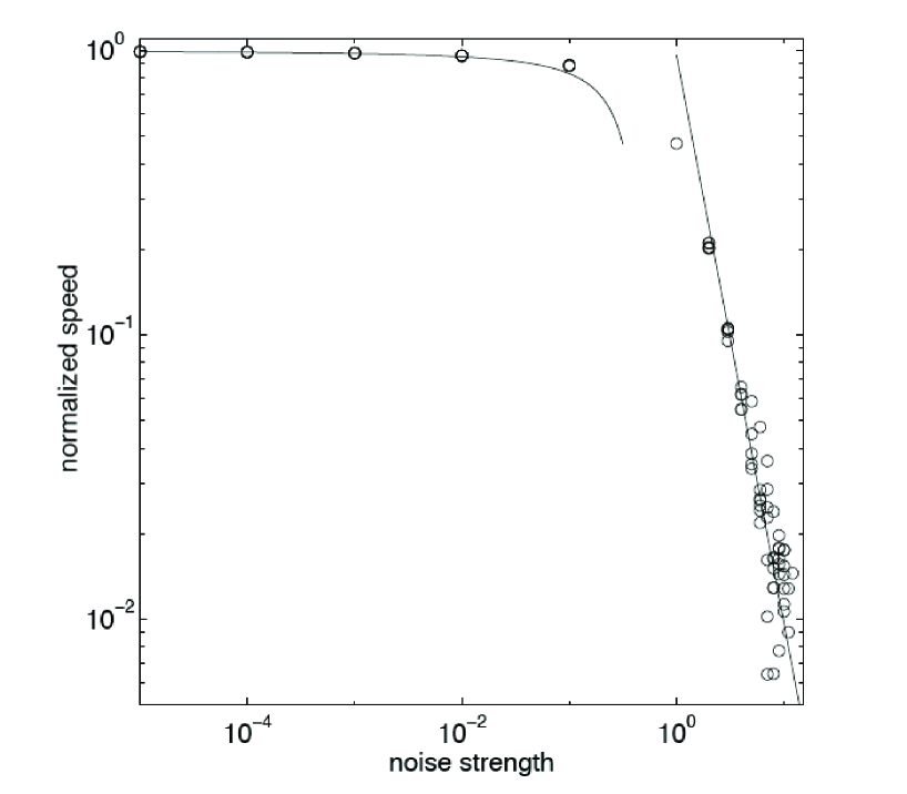
Figure 2: Average wave speed as a function of the noise for the sFKPP equation. Vertical axis: $v/v_{c}$ is the average traveling wave speed normalized to the speed $v_{c}=2$ of the deterministic FKPP equation; Horizontal axis: dimensionless noise strength; Dots: numerical results; Left line: weak noise analytic prediction; Right line: strong noise prediction. One observes (and may derive maximal ) a maximal speed around a noise strength of order 10. The figure is from ref.mueller .

IV.3 Stochastic traveling waves : strong noise

When the noise strength is tuned to increase, one observes a strong decrease of the average wave velocity, with a neat change of regime in the vicinity of a (normalized) noise strength of order one, see Fig.2. Following Ref.strong , the overall properties of the strong noise regime are as follows

The solution of equation (10) is a stochastic average of traveling waves at an average speed

$$v=\frac{2}{\zeta^{2}}\sim\ \frac{4\pi r_{s}(t)}{\epsilon^{2}}\ ,$$ (25)

where $\zeta$ is the normalized noise strength defined in (20). Hence the saturation scale $r_{s}$ follows from the equation

$$v\equiv\frac{dr_{s}}{dt}=\ \frac{4\pi r_{s}(t)}{\epsilon^{2}}\Rightarrow\ r_{s}(t)\propto e^{4\pi t/\epsilon^{2}}\ ,$$ (26)

where the rapidity dependence of the radial noise plays the important role. Note that the limiting speed condition anyway requires $v<v_{c}\equiv 2$ and thus from (25) ${4\pi r_{s}(t)}<{\epsilon^{2}}.$ Hence the exponential behavior of (26) must break down before the time evolution reaches the limit defined by ${2\pi}\ e^{4\pi t/\epsilon^{2}}\to{\epsilon^{2}}.$ In fact, due to the rapidity decrease of the effective noise $\zeta$ of (20), the strong noise regime transforms progressively into the weak noise one, following from right to left the velocity curve depicted in Fig.2.

In the strong noise regime, there exists strong an analytic solution for the average solution of the evolution equation (10), namely

$$\left\langle{U(t,r)}\right\rangle = \frac{1}{2}\ {\rm erfc}\left(\frac{r-r_{s}(t)}{2\sqrt{t}}\right)$$ (27)

$$= \frac{1}{2\sqrt{\pi t}}\int_{-\infty}^{\infty}dr\,\theta(\tilde{r}-r)\exp{-\frac{(\tilde{r}-r_{s}(t))^{2}}{4t}}\ ,$$

where ${\rm erfc}(x)$ is the complementary error function.

This result confirms the decrease of the velocity with increasing noise strength. It contrasts with the speed obtained in the weak noise limit by perturbative analysis around the F-KPP speed $\simeq 2-\pi^{2}|\log(2\zeta^{2})|^{-2}.$ The expression (27) shows that the amplitude could be obtained from a superposition of step functions around $r_{s}=v\ t$ with a Gaussian form of width $\sqrt{2Dt}$. The interesting point here lies in the dispersion coefficient: in the weak-noise analysis, it behaves like $|\log(2\zeta^{2})|^{-3}$. We have thus shown that the dispersion goes to a constant value $2$ when the noise becomes strong.

V The Pomeron as a circular traveling wave

Let us investigate the implications of the traveling wave properties on the soft Pomeron, within the framework that the soft interaction dynamics at high energies be governed by a “supercritical” bare Pomeron input. As we have shown in the previous theoretical sections, the circular traveling wave solutions are expected to appear due to the combined effect of the high energy evolution and of unitarity, which we will assume to be saturated. Our analysis will be concerning the asymptotic regime of the circular traveling waves, leaving for further study the transition to this regime.

We have seen that the evolution towards the saturation limit may depend on the non-linear terms, see Eq.(18). Those terms may be physically more complicated than the single quadratic term of Eq.(5). Hence we will focus on the “universal predictions”, $e.g.$ those which do not depend on the initial conditions and/or the structure of the non-linear damping. On the contrary, the parameter $\kappa,$ which is not fixed by the unitarity constraints, is the relevant parameter, playing an essential role in the Pomeron properties.

V.1 “Phase diagram” as a function of noise

The first step is to discuss which evolution regime we have as a function of $\kappa.$ For this sake, the noise strength (20) can be conveniently written, restoring the Pomeron variables (7)

$$\zeta^{2}=\frac{\epsilon^{2}}{2\pi r_{s}}\equiv\frac{\kappa}{2\pi}\frac{\sqrt{\alpha^{\prime}\mu}}{b_{s}}\ .$$ (28)

It is important to note the following feature of the noise strength directly related to the (2+1)-d property of the RFT problem: it decreases together with the expansion of the impact-parameter disk and thus evolves towards weaker noise. However, this decrease, being governed by the evolution of the disk may be slow.

The basic relation we will get comes from the structure of the wave speed reproduced in Fig.2. It is obtained for the 1-d case, but it happens to be indicative also for the radial case, whose universal properties are essentially similar, as we shall see. In Fig.2, one may distinguish how the three different regimes we have analyzed in the previous sections, namely the zero, weak and strong noise respectively, can be identified on the plot where the $\kappa$-dependent normalized speed $v_{\kappa}/v_{c}$ is displayed as a function of the normalized noise strength $\zeta$. With our notations and using (28), we write by straightforward relations

$$\frac{v_{\kappa}}{v_{c}}\equiv\frac{1}{v_{c}}\ \frac{dr_{s}}{dt}=\frac{1}{2\sqrt{\alpha^{\prime}\mu}}\ \frac{db_{s}}{dY}=\frac{\kappa}{4\pi}\ \frac{1}{\zeta^{2}}\ \frac{2db_{s}}{b_{s}dY}\ ,$$ (29)

where we have denoted $v_{\kappa}\equiv\frac{dr_{s}}{dt}$ the actual wave front velocity and $v_{c}=2,$ the deterministic critical speed. Note that we have made use of (28) to substitute the bare Pomeron parameters $\sqrt{\mu\alpha^{\prime}}$ by its expression in terms of the normalized noise. Our final expression thus writes

$$\frac{v_{\kappa}}{v_{c}}=\left[\frac{\kappa\delta}{4\pi}\right]\ {\zeta^{-2}}\ ,$$ (30)

where $\delta\equiv 2{db_{s}}/{b_{s}dY}=d\log{\cal A}/{dY},$ where ${\cal A}=\pi b^{2}_{s}$ is the area of the effective impact-parameter disk for the collision. The obtained expression shows directly how the noise strength $\kappa$ parametrizes the normalized-speed $vs.$ normalized-noise relation depicted in Fig.2. It allows one to relate the “phase diagram” defining the different regimes of the radial sFKPP equation to a physical soft Pomeron feature, namely the exponent $\delta$ of the expanding disk area ${\cal A}$.

When interpreting Fig.2, one may distinguish the different regimes as follows using relation (29):

• The weak noise regime:

  $$\!\!\!\!\!\!\!\!\!\!\!\!\zeta\leq{10^{-1}}\quad\quad.9\leq\frac{v_{\kappa}}{v_{c}}\leq 1.\quad\quad\quad\ \frac{\kappa}{4\pi}\leq\frac{10^{-2}}{\delta}\quad\quad 2\sqrt{\mu\alpha^{\prime}}\lesssim\ {\frac{1}{2}}{\delta b_{s}}=\ \frac{db_{s}}{dY}\ .$$ (31)

• The strong noise regime:

  $$\ \quad\zeta\gtrsim 1.4\quad\quad\quad\zeta^{-2}=\frac{v_{\kappa}}{v_{c}}\ \lesssim.5\quad\quad\ \ \ \frac{\kappa}{4\pi}=\frac{1}{\delta}\quad\quad\quad\ 2{\sqrt{\mu\alpha^{\prime}}}\sim\frac{\zeta^{2}}{2}\ {\delta b_{s}}={\zeta^{2}}\frac{db_{s}}{dY}\gtrsim 2\frac{db_{s}}{dY}\ ,$$ (32)

  where we made use of the exact relation at strong noise (25). To complete the picture, one adds

• The zero noise regime:

  $$\!\!\!\!\!\!\!\!\!\!\!\!\!\!\!\!\zeta\lll 1\quad\quad\quad\quad\frac{v_{\kappa}}{v_{c}}\sim 1\quad\quad\quad\quad\quad\frac{\kappa}{4\pi}\sim\ 0\quad\quad\quad{2\sqrt{\mu\alpha^{\prime}}}\sim\ \frac{1}{2}\ {\delta b_{s}}=\ \frac{db_{s}}{dY}\ .$$ (33)

• The middle noise regime:

  $$\!\!\!\!\!\!\!\!\!\!\!\!\!\!\!\!\!\!\!\!\!\!\!\!.1\leq\zeta\leq 1.5\quad\quad.2\leq\ \frac{v_{\kappa}}{v_{c}}\ \leq.9\quad\quad\frac{10^{-2}}{\delta}\leq\frac{\kappa}{4\pi}\leq\frac{1}{\delta}\quad\quad\quad\ \ \frac{db_{s}}{dY}\leq{2\sqrt{\mu\alpha^{\prime}}}\leq\ 2\frac{db_{s}}{dY}\ .$$ (34)

We see from relations (31-34) that the parameter $\kappa$ plays the role of the order parameter of the RFT. Once given the physical observable $\delta$, one knows the phase ($cf.$ evolution regime) of the system from the determination of $\kappa.$ In particular for the original RFT action (1), the phase is completely specified by $\delta.$ Note also that the “bare” parameter $2\sqrt{\alpha^{\prime}\mu}$ corresponding to the maximal critical speed of the disk relates to $b_{s}\delta/2\equiv\frac{db_{s}}{dY}$ which is a “dressed” parameter in terms of a field theory.

The question of determining the soft Pomeron properties thus boils down to the determination of $\delta.$ We postpone a detaileed phenomenological study for the future, but it is not too difficult to evaluate the order of magnitude of $\delta.$ Indeed, if the black disk limit would have been nearly reached, one would expect a geometrical cross-section $\sigma_{tot}\propto{\cal A}=\pi b^{2}_{s}$ and thus $\delta\sim d\log\sigma_{tot}/dY\sim.08$ where the last number is the well-known popular determination donach . This value for $\delta$ should be considered as a maximum at present energies, since the black disk limit seems not to be fully reached (see, $e.g.$, models , where one obtains smaller values of order $\delta\sim(1-3)10^{-2}$). as an example in appendix C we show the phase diagram characteristics when choosing the conservative values of $\delta\sim 10^{-2}$ and $b_{s}\sim 1\ {\rm fermi=5\ GeV}^{-1}.$

In any case, one interesting remark is that for the whole range $\delta\in[1-8]10^{-2},$ the original RFT with $\kappa=1$ seats within the limit of the weak noise region. By comparison, the order parameter $\kappa$ takes a factor 100 in the interval between the weak and the strong noise regimes. Such high values of $\kappa$ are not it a priori forbidden, even if far from the original RFT action with a single triple Pomeron coupling. We will discuss in conclusion a possible QCD interpretation of these large values of $\kappa$.

V.2 Properties of the “wave front”

V.2.1 An expanding impact-parameter disk

Having now identified the phase diagram of the RFT solutions, we are able to discuss the characteristic features of the soft Pomeron as a circular traveling way by recasting the results of section II ($resp.$ III) for the deterministic ($resp.$ stochastic) traveling waves in terms of the physical variables through the relations (7).

As a general result, valid in all cases, we find that the front of the traveling wave is situated around the impact-parameter value

$$b_{s}(Y)=\sqrt{\alpha^{\prime}/\mu}\ r_{s}(t=\mu\ Y)\ .$$ (35)

The expanding impact-parameter disk is thus related to the increasing function $r_{s}(t).$ This is the analogue of the rapidity-dependent “saturation scale” GW discussed also in the framework of QCD traveling waves munier . Let us examine the equivalent “saturation scale” of the supercritical Pomeron. As we have seen previously, it depends on the phase diagram. Following Eqs.(13), (21) and (25) respectively, we obtain

$$b_{s}(Y)-b_{s}(Y_{0}) = 2\sqrt{\alpha^{\prime}\mu}\ \left[(Y\!-Y_{0})-\frac{1}{\mu}\ {\log\frac{Y}{Y_{0}}}+\cdots\right],\ {\rm for\ zero\ noise}$$

$$b_{s}(Y)-b_{s}(Y_{0}) = 2\sqrt{\alpha^{\prime}\mu}\ (Y\!-Y_{0})\ \left[1-\frac{\pi^{2}}{2\log^{2}\left(2\zeta^{-2}\right)}+\frac{3\pi^{2}\log\log\left(2\zeta^{-2}\right)}{\log^{3}\left(2\zeta^{-2}\right)}+\cdots\right],\ {\rm for\ weak\ noise}$$

$$b_{s}(Y) = b_{s}(Y_{0})\quad\exp{\left[\frac{4\pi}{\kappa}\ (Y\!-Y_{0})\right]},\ {\rm for\ strong\ noise}.$$ (36)

The middle-noise regime does not posses an analytic expression but its numerical implementation is possible and shown (in the reduced variables) on Fig.2. The dots $(\cdots)$ stand for sub-leading and/or non-universal higher order terms. Note that the constant terms implied by the initial condition at $Y\!=Y_{0}$ are also naturally not constrained by universality. The validity of relations (36) thus require a large enough interval $Y\!-Y_{0}.$ For all cases one finds from (36) that the disk expands with rapidity. For the “zero noise” and “weak noise” cases the asymptotic velocity is $2\sqrt{\alpha^{\prime}\mu},$ which is the critical velocity, and thus driven by the deterministic equation. The situation is different at “strong noise” where the solution is still moving linearly with rapidity $Y$ but with a velocity governed by the order parameter $\kappa$.

For the “zero noise ” and “weak noise” cases, we have thus identified new universal terms not depending on the initial conditions nor on the specific non-linear damping terms. The existence of an universal rapidity expansion due to the supercritical Pomeron is, to our knowledge, a new result allowed by the Langevin formulation of the RFT and its traveling wave solutions. Moreover they appear to be quite different depending on non trivial phase diagram: in the deterministic case, the first (negative) correction to the radius $b_{s}\propto Y$ behaves like $\log Y$, while it is of order $Y\log^{-2}Y$ for “weak noise”, and thus a priori quite more important than in the deterministic case.

For “strong noise”, the obtained exponential behavior would not lead ultimately to a violation of the Froissart bound since the rise is tamed by the boundary of the strong noise regime. From (28) and the relations (32), one has

$$\zeta^{-2}=\frac{2\pi b_{s}}{\kappa\sqrt{\alpha^{\prime}\mu}}=v_{\kappa}/v_{c}\lesssim.5\quad\Rightarrow\quad b_{s}\ \lesssim\frac{\kappa}{4\pi}\ \sqrt{\alpha^{\prime}\mu}\ .$$ (37)

In fact this limit on the impact-parameter disk reflects the $Y$-dependence of the noise strength and thus the evolution from strong noise towards weak noise through an intermediate middle-noise regime. Interestingly enough, this would mean for the radius (and thus for the cross-section near the black disk limit) a gradual transition from an exponential towards a squared logarithmic behavior in rapidity and thus an asymptotic restoration of the Froissart bound.

V.2.2 Impact-parameter Scaling

The scattering amplitude is related to the front profile of the dominant asymptotic traveling wave solution through

$$T(Y,b)=U\left(t=\mu\ Y,\ r=\sqrt{\frac{\mu}{\alpha^{\prime}}}\ b\right)\ ,$$ (38)

at least in the region where universal results apply. $U(t,r)$ being given by formulas (11), (24) and (27) respectively, one obtains

$$T(Y,b) \sim T\left\{b-b_{s}(Y)\right\},\ {\rm for\ zero\ noise}$$

$$T(Y,b) \sim T\left\{\frac{b-b_{s}(Y)}{D_{w}(Y)\sqrt{\alpha^{\prime}(Y\!-Y_{1})}}\right\},\ {\rm for\ weak\ noise}$$

$$T(Y,b) \sim \ T\left\{\frac{b-b_{s}(Y)}{D_{s}\sqrt{\alpha^{\prime}(Y\!-Y_{1})}}\right\},\ {\rm for\ strong\ noise}\ ,$$ (40)

where the values of the front scales $b_{s}(Y)$ have to be chosen from (36) for each corresponding individual regime. $D_{w}$ and $D_{s}$ are the dispersion parameters for weak and strong noise respectively. We have introduced a rapidity scale $Y_{1}$ which denotes the effective rapidity where the dispersion of the noisy traveling waves becomes sizable. Indeed, numerical simulations for the QCD case gregory show that such a threshold do exist. Below that threshold the scaling is similar to the zero noise case. From (23) and (27), one finds

$$D_{w}=\frac{2\pi^{2}}{3\log^{3}\left[2\zeta^{-2}\right]}=\frac{2\pi^{2}}{3\log^{3}\left[4\pi b_{s}/\kappa\sqrt{\alpha^{\prime}\mu}\right]}\ ;\quad\quad D_{s}\equiv 2\ .$$ (41)

It is clear that the dispersion parameter $D_{w}\propto 1/\log^{3}Y$ may be quite small and thus one would then recover the same scaling as the zero-noise regime, but with the different weak-noise evolution $b_{s}(Y)$. Moreover the dispersion is proportional to $\sqrt{}\alpha^{\prime}$ which may be small even for a sizable value of $\sqrt{\alpha^{\prime}\mu}$ for larger $\mu.$

V.2.3 Front profile

In the regions where there exists a universal form of the wave front profile, $i.e.$ within and forward to the wave front (the previously called “wave interior” and “leading edge” regions), one finds from formulas (11), (22) and (27) respectively,

$$T(Y,b) \sim (b-b_{s})\ \exp{\left\{-\sqrt{\frac{\alpha^{\prime}}{\mu}}\ (b-b_{s})-\frac{\left(b-b_{s}\right)^{2}}{4\alpha^{\prime}(Y\!-Y_{0})}\right\}},\ {\rm for\ zero\ noise}$$

$$T(Y,b) \sim \text{erfc}\left\{\frac{b-b_{s}}{D_{w}\sqrt{\alpha^{\prime}(Y\!-Y_{1})}}\right\}+\exp{\left(\frac{\mu\ D_{w}^{2}{(Y\!-Y_{1})}}{4}-\sqrt{\mu/\alpha^{\prime}\ (b-b_{s})}\right)}\ \times$$

$$\ \ \times\ \left\{2-\text{erfc}\left(\frac{b-b_{s}}{D_{w}\sqrt{\alpha^{\prime}(Y\!-Y_{1})}}-\frac{D_{w}\sqrt{\mu(Y\!-Y_{1})}}{2}\right)\right\},\ {\rm for\ weak\ noise}$$

$$T(Y,b) \sim \text{erfc}\left\{\frac{b-b_{s}}{2\sqrt{\alpha^{\prime}(Y\!-Y_{1})}}\right\},\ {\rm for\ strong\ noise}\ ,$$ (42)

where $D_{w},D_{s}$ were given in (41).

Some comments are in order about the front profiles. We may note that $T(b,Y)$ for the zero noise case goes to zero with $b-b_{s},$ corresponding to the way how saturation is imposed as an “absorbing condition” absorb to the leading-edge approximations of the traveling waves’ tails. Around and below $b=b_{s}$ the solutions get corrections to the spurious zero. However, these corrections (see, $e.g.$ (16)) are more dependent on the specific form of the nonlinear terms of the equation.

Note also that the diffusive scaling (24) is exact for the strong noise case and with exact dispersion parameter $D_{s}\equiv 2.$ It comes from an exact solution of the statistical mechanic picture strong . Indeed, the strong noise regime can be interpreted as the stochastic superposition of traveling waves of the simple form $\theta(b-b_{s}),$ suggested by Eq.(27). Moreover, at strong noise, the average solution is dominated by the strongest fluctuations, together with all correlators, as shown in strong .

VI Conclusions

We can summarize our results as follows:

i) Reggeon Field Theory, when the bare Pomeron is “supercritical”, can be formulated as a stochastic equation which is in the same “universality class” than the 2-dimensional version of the stochastic Fisher and Kolmogorov-Petrovsky-Piscounov equation. In this framework, “time” corresponds to a rapidity evolution $Y-Y_{0}$ and “space” to the 2-d impact-parameter $\vec{b}$ of the hadronic collision.

ii) Thanks to the mapping to the 2d-sFKPP equation, one is able to find the asymptotic and certain subasymptotic solutions of the RFT which were beyond reach of the purely field theoretical methods used in the past. These solutions possess an appealing “universality ” property, which means that they do not depend either from the initial conditions or on the peculiar form of the non-linear terms ensuring the unitarity constraint on the elastic amplitude.

iii) To our knowledge, it is yet the only example of a supercritical Pomeron theory preserving an universal behavior of the amplitude. Usually, the factorisation property of a Pomeron as a Regge pole, on which relies the standard universality arguments (see, $e.g.$ donach ), is expected to be washed out by interactions for a RFT based on a supercritical Pomeron. This “universality” property is recovered in a very different way, since it comes from a dynamical mechanism based on the “critical” phenomenon associated to the formation of circular traveling waves.

iv) The “universality class” property remains valid when the splitting and merging Pomeron vertices are of ratio $\kappa\neq 1,$ which was the RFT value based on the unique triple Pomeron coupling. Indeed, $\kappa,$ which is a measure of the strength of the “Pomeron loop” contribution, plays the role of the “order parameter” in the phase diagram of the RFT. Hence the original RFT (with $\kappa=1$) lies in a specific phase of the diagram. A rough but realistic estimate (assuming RFT to be physically applicable) places the original RFT in the “weak noise” regime of sFKPP. However, thhis choice is not dictated by a theoretical constraint. The full phase diagram should allow a model-independent discussion of this degree of freedom, if compared directly with the phenomenology.

v) More generally, depending on the dimensionless noise strength $\kappa$ the phase diagram is shown to lead to three specific phases corresponding respectively to zero noise ($\kappa=0$), weak noise ($\kappa={\cal O}(1)$) and strong noise ($\kappa={\cal O}(100)$), (plus an intermediate middle noise one (${\cal O}(1)\lesssim\kappa\lesssim{\cal O}(100)$), for which explicit asymptotic regimes of solutions are obtained in the front and in the tail of the impact-parameter disk. Some other results, valid in the whole range are obtained in the case of triple-Pomeron coupling.

There are intringuing theoretical lessons to be drawn from our results The striking theoretical feature of the approach to the RFT through the mapping to the 2-dimensional sFKPP equation is its ability to avoid the complications of an usual field theory formulation in the case of a “supercritical” bare Pomeron. Indeed, if at first a “critical” Pomeron theory for which the renormalization group exists raised some hope (see $e.g.$ abarbanel ) it led to unphysical results for hadronic reactions such as total cross-sections behaving as $Y^{1/12}.$ For a “supercritical Pomeron” the field theoretical methods, interesting as they may be (see $e.g.$ parisi ), appeared to be technically complex with difficulties to conveniently handle the solutions. It thus seems that the traveling wave methods developped in the present study are well suitable for avoiding the obstacles. It is quite remarkable that, even a domain dominated by very large “quantum loop” contributions such as the strong noise phase discussed here, can be handled in a quite economic way.

It is useful to list a series of interesting theoretical subjects which lie beyond the present study. One first problem is to get rid of the approximations made for the derivation of the solutions, the main one being to have replaced in the original equation (9) the $r$-dependent coefficients by their value on the wave front $r_{s}.$ It would improve the analysis to solve, even numerically, the original equation to check the validity of the approximation.

The question of the azimuthal dependence of the noise is perhaps challenging and thus interesting. Indeed, It could a priori be possible that azimuthal symmetry be recovered $after$ averaging over the noise. However, it is known from the study of a plane front kessler that instabilities may be created by the fluctuations beyond some threshold. It is reasonable to expect that the unitarity constraint should cut-off such inhomogeneities, leaving the purely radial solution valid. For non azimuthally symmetric variables, this is not so obvious and studies $e.g.$ related to the “supercritical Pomeron” in diffraction dissociation or for particle production could lead to some interesting problems, such as the noisy structure of the diffraction disk parisi2 .

Finally, it would be natural and interesting to address the question of the relation of our results with QCD. A priori, there is a long way to go from an effective and thus “macroscopic” theory of Pomeron interactions to a “microscopic” point-of view based on quark and gluon interactions. Perhaps a tentative approach would be to notice that the RFT can be considered using the “hard” Pomeron as an input and thus depending of the value of a QCD coupling constant $\alpha_{S}$. Since, finally, the only order parameter we have is $\kappa,$ this would mean that this parameter should be considered depending on $\alpha_{S}.$ It is interesting to note that the strong noise regime leads to the rapidity dependence $b_{s}\propto e^{4\pi/\kappa}.$ A “hard” pomeron behaviour which value of intercept is proportional to $\alpha_{S}$ would lead to choose $\kappa\propto 1/\alpha_{S}.$ Hence a “perturbative” property for QCD would be in relation with a highly quantum regime (large Pomeron loops strength $\kappa$) in terms of RFT. By contrast a quasi-classical regime of RFT (zero or weak noise, small $\kappa$) would be associated to a large effective coupling constant of order $\alpha_{S}\sim 1/\kappa.$ This speculative but intringuing “duality property” deserves certainly some interest.

Appendix A: Derivation of the radial “leading edge”

In the following we shall restrict our analysis to radial amplitudes, $i.e.$ depending only on the radial coordinate $r=|\vec{r}|.$ One starts with

$$\frac{d}{dt}\ U\left(t,r\right)=\partial_{rr}\ U+\frac{1}{r}\ \partial_{r}\ U+\ U-\ U^{2}\ .$$ (43)

Let us introduce, following a similar procedure for the 1-dimensional problem brunet ; beuf , the ansatz

$$U\left(t,s=r\!-\!v_{c}t\right)\ \propto\ \exp{\left[-\gamma_{c}(s+c(t))\right]}\ t^{\alpha}\ G\left(\frac{s+c(t)}{t^{\alpha}}\right)\ ,$$ (44)

where $v_{c}$ ($resp.\ \gamma_{c}$) are the critical wave velocity ($resp.$ critical slope) of the traveling wave front. This ansatz is for describing the universal behavior of the wave in the leading edge region forward to the front wave1 .

Inserting (44) in the equation (43) and neglecting the small contribution from the nonlinear term to the leading edge, we can verify the equation for the dominant terms of the time expansion. the different terms give:

$$\frac{1}{U}\ \frac{dU}{dt} = \left(\gamma_{c}-t^{-\alpha}\frac{G^{\prime}}{G}\right)v_{c}-\gamma_{c}c^{\prime}(t)+\frac{\alpha}{t}+\alpha t^{-\alpha-1}[s+c(t)]\frac{G^{\prime}}{G}+...$$

$$-\frac{1}{U}\frac{\partial_{s}U}{r} = \left(\gamma_{c}-t^{-\alpha}\frac{G^{\prime}}{G}\right)\left[\frac{1}{s+v_{c}t}\right]=\left(\gamma_{c}-t^{-\alpha}\frac{G^{\prime}}{G}\right)\left[\frac{1}{v_{c}t}\right]+...$$

$$\frac{1}{U}{\partial_{ss}U} = \left(\gamma_{c}-t^{-\alpha}\frac{G^{\prime}}{G}\right)^{2}+t^{-2\alpha}\left[\frac{G^{\prime\prime}}{G}-\frac{G^{\prime\prime 2}}{G^{2}}\right]+...\ ,$$ (45)

where the dots $(...)$ indicate irrelevant sub-dominant contributions.

Order by order in the late time expansion we get the following relations

$$\gamma_{c}v_{c}=(\gamma_{c})^{2}+1\quad \Rightarrow {\rm(order}\ t^{0})$$

$$v_{c}=2(\gamma_{c})\quad \Rightarrow ({\rm order}\ t^{-\alpha})$$

$$0=\alpha\gamma_{c}\beta_{c}-\alpha-\frac{\gamma_{c}}{v_{c}}+\alpha z\frac{G^{\prime}}{G}+\frac{G^{\prime\prime}}{G}\quad \Rightarrow ({\rm order}\ t^{-2\alpha})\ ,$$ (46)

with $z\equiv(s/t^{-\alpha})$ fixed and finite and $c(t)\equiv\beta_{c}\log t.$ Hence we get the values of the critical parameters $\alpha=1/2;\gamma_{c}=1;v_{c}=2.$ The last equation of (46) now reads

$$0=(\beta^{*}-1)\ G(z)+\frac{z}{2}\ G^{\prime}(z)+G^{\prime\prime}(z)\ .$$ (47)

The condition $G(z)\to z$ when $z\to 0,$ necessary to match with the scaling region (called the “wave interior” in wave1 ), leads to $\beta_{c}=5/2$ and $G(z)\propto z\ e^{-z^{2}/4}$. One thus finally gets

$$U^{l.e.}(r\!-\!r_{s},t) \sim \ \exp{\left[-(r-r_{s})\right]}\ (r-r_{s})\ \exp{\left(-\frac{1}{4}\ \left[\frac{r-r_{s}}{t^{1/2}}\right]^{2}\right)}\ ,$$

$$r_{s} = 2t-2\log t$$ (48)

where ${l.e.}$ stands for leading edge and $r_{s}$ is the average moving position of the wave front (or “saturation scale” in the language of QCD munier ). Note that the form of the front is identical to the one obtained in the 1-dimensional problem brunet ; munier but the saturation scale is $r_{s}=s-c(t)+1/2=2t-{\bf 2}\log t$ (instead of $r_{s}=s-c(t)+1/2=2t-{\bf\frac{3}{2}}\log t,$) and thus slower by a logarithmic factor ${\bf\frac{1}{2}}\log t.$ This shift can be interpreted (and checked) derrida as resulting from the superposition of the “curvature contribution” of the 2-dimensional problem with the dynamical slowing down of the 1d FKPP solutions.

Appendix B: Derivation of the radial “wave interior”

Let us introduce the formula (15) into the equation (10) and expand in powers of $\Delta^{-2},$ one gets

$$0 = \left[\frac{v(t)}{\Delta}+\frac{1}{\Delta\int^{t}dt^{\prime}v(t^{\prime})}\right]U^{\prime}_{0}+U_{0}-U_{0}^{2}$$

$$0 = \left[\frac{v(t)}{\Delta}\right]U^{\prime}_{1}+U^{\prime\prime}_{0}+\left(1-2U_{0}\right)U_{1}\ ,$$ (49)

where, one has replaced $\frac{1}{r}\ \partial_{r}U\to\frac{1}{\int^{t}dt^{\prime}v(t^{\prime})}\ \partial_{r}U$ in (10) since the difference is ${\cal O}(1)\ll\Delta t$ in the wave interior.

In fact, we choose $\Delta=cst.$ such that $\left[\frac{v(t)}{\Delta}+\frac{1}{\Delta\int^{t}dt^{\prime}v(t^{\prime})}\right]=1,$ leading by simple integration to the equation

$$r_{s}\equiv\int^{t}dt^{\prime}v(t^{\prime})\equiv\Delta t-\frac{1}{\Delta}\log\left(\Delta r_{s}\right)\sim\Delta t-\frac{1}{\Delta}\log\left(\Delta^{2}t-1\right)$$ (50)

at large time. Solving the simple nonlinear equation of the first line of (49) one easily gets

$$U_{0}=\frac{1}{1+e^{\frac{r-r_{s}}{\Delta}}}\equiv\frac{1}{1+e^{z}}\\ .$$ (51)

Knowing the solution for $U_{0},$ it is not too difficult to solve the linear equation, second line of (49), obtaining with the appropriate boundary conditions

$$U_{2}=\frac{e^{z}}{\left(1+e^{z}\right)^{2}}\ \log{\frac{\left(1+e^{z}\right)^{2}}{4e^{z}}}\ .$$ (52)

Appendix C: RFT phase diagram for $\delta=2\ 10^{-2}$ and $b_{s}\sim 5\ {\rm GeV}^{-1}$

• The zero noise regime:

  $$\!\!\!\!\!\!\!\!\!\!\!\!\!\!\!\!\zeta\ll 1\quad\quad\quad\frac{v_{\kappa}}{v_{c}}\sim 1\quad\quad\quad\quad\ \kappa\ll\ 1\quad\quad\quad{\sqrt{\mu\alpha^{\prime}}}\sim\ .025\ {\rm GeV}^{-1}\ .$$ (53)

• The weak noise regime:

  $$\zeta\leq{10^{-1}}\quad\quad.9\leq\frac{v_{\kappa}}{v_{c}}\leq 1\quad\quad\quad\ \kappa\leq{2\pi}\quad\quad{\sqrt{\mu\alpha^{\prime}}}\lesssim.025\ {\rm GeV}^{-1}\ .$$ (54)

• The strong noise regime:

  $$\ \quad\quad\quad\quad\zeta\gtrsim 1.4\quad\quad\quad\zeta^{-2}=\frac{v_{\kappa}}{v_{c}}\ \lesssim.5\quad\quad\ \kappa=200\ \pi\quad\quad\quad\ {\sqrt{\mu\alpha^{\prime}}}\sim\frac{\zeta^{2}}{4}\ {\delta b_{s}}\sim.025{\zeta^{2}}\ \gtrsim.05\ {\rm GeV}^{-1}\ ,$$ (55)

• The middle noise regime:

  $$\!\!\!\!\!\!.1\leq\zeta\leq 1.5\quad\quad\quad.2\leq\ \frac{v_{\kappa}}{v_{c}}\ \leq.9\quad\quad\quad\quad\ 2\pi\leq\kappa\leq 200\ \pi\quad\quad\quad\ .025\ {\rm GeV}^{-1}\leq{\sqrt{\mu\alpha^{\prime}}}\leq\ .05\ {\rm GeV}^{-1}\ .$$ (56)

Appendix D: Phenomenological Remarks

a) Scaling in impact-parameter. The main property of the traveling wave solution is its scaling structure in impact-parameter. On a phenomenological ground, assuming for simplicity a purely imaginary elastic amplitude, one obtains a scaling property of the elastic amplitude considered as a function of impact-parameter and energy. One may write $ImT_{el}(Y,b)\sim T(b-b_{s}),$ where $b_{s}$ describes an expanding scattering disk ${\cal A}=\pi b^{2}_{s}$ possessing universal slowering corrections. Note that it is the “soft interaction” version, in the variables $(Y,b)$, of a the similar “geometric scaling” golec of the “hard interaction” encountered in deep-inelastic scattering and involving instead the $(Y,\log Q^{2})$ variables.

As discussed in the paper, we expect scaling to stay approximately valid at weak noise, at least before a fully realized stochastic regime takes place where $ImT_{el}(Y,b)\approx T\left\{\frac{b-b_{s}}{D\sqrt{Y}}\right\}.$ However, in this case, some non negligible corrections are expected to appear also in the disk radius, see (36).

b) Total cross sections

The existence of an expanding disk in impact-parameter given by Eqs.(36) may have a direct consequence on forward scattering amplitudes, and through unitarity, on the total cross-section at high energy. Indeed, taking as an example the ideal geometric relation $\sigma_{tot}\propto{\cal A}$ one finds for the zero noise case in appropriate units and for the dominant terms at asymptotic $Y$

$$\sigma\to\left\{Y^{2}-\frac{2Y\log Y}{\mu}+\cdots\right\}\ .$$ (57)

Eq.(57) saturates the $Y^{2}$ behavior given by the Froissart bound, and thus restores unitarity. However, our prediction is the existence of a “universal” $Y\log Y$ correction term with strength governed by the bare Pomeron intercept $\mu.$ It is directly related to the correction term of the traveling wave speed (13).

Note that the result for the stochastic regime may be significantly different, namely

$$\sigma(Y) \to Y^{2}\left\{1-\frac{2\pi^{2}}{\log^{2}{\left(\frac{8\pi Y}{\kappa}\right)}}+\cdots\right\},\ {\rm for\ weak\ noise}$$

$$\sigma(Y) \to \ \exp{\frac{8\pi\ Y}{\kappa}},\ {\rm for\ strong\ noise}\ ,$$ (58)

The results (58) call for comments. In the weak noise regime, it is clear that the stochastic corrections depending on the parameter $\kappa$ are of order $1/\log^{2}Y$ and thus significantly more important than the deterministic ones of order $\log Y/Y,$ see formula (57). Hence the Pomeron loop effects are expected, if their coupling $\kappa$ in the supercritical Pomeron scenario is effective, to have an observable effect.

At strong noise, the behavior of the cross-section is entirely governed by the noise, with its characteristic parameter $\kappa.$ It is interesting to note that, if the phenomenological soft Pomeron of Ref.donach with intercept $1.08$ is attributed to a strong noise scenario, it would correspond to $\kappa\sim 100\pi,$ which is discussed in the previous section III. Note that anyway the noise strength decreases like $1/\sqrt{Y}$ and the strong noise regime will transform into the middle if not the weak noise one after some rapidity evolution. Hence the apparent violation of the Froissart bound will not be maintained at high enough energy.

c) Modification of the large $b$ behaviour

It is interesting to study how the traveling wave behavior modifies the transfer momentum dependence of the elastic cross-section and thus the diffraction peak. Indeed, as we have seen previously, starting with an initial condition which is Gaussian in impact-parameter, the asymptotic traveling wave solution drives the solution of the evolution equation to a different, “universal” form ($e.g.$ independent from the initial condition and the precise form of the non-linear damping terms in the equation). By Fourier transform, this evolution should change the structure of the amplitude in momentum transfer, and thus modify the diffraction peak.

For an example we will start with the expression of the wave front in the “leading edge” domain at zero noise, formula (13). With some rearrangement of terms one can write

$$T(Y,b)\propto(b-b_{s})\ \exp{\mu(Y\!-Y_{0})}\ \exp{-\frac{\left[b+2\sqrt{\frac{\alpha^{\prime}}{\mu}}\ \log(\mu(Y\!-Y_{0}))\right]^{2}}{4\alpha^{\prime}(Y\!-Y_{0})}}\ .$$ (59)

In Formula (59), we note that, apart the linear prefactor, the exponential behavior dominant at large $Y$ boils down to the following modification

$$\exp\left\{\mu(Y\!-Y_{0})-\frac{b^{2}}{4\alpha^{\prime}(Y\!-Y_{0})}\right\}\to\exp\left\{\mu(Y\!-Y_{0})-\frac{{\bar{b}}^{2}}{4\alpha^{\prime}(Y\!-Y_{0})}\right\}\ ,$$ (60)

where

$$\bar{b}=b+2\sqrt{\frac{\alpha^{\prime}}{\mu}}\log(\mu(Y\!-Y_{0})).$$

One recognize in the left-hand of (60) the solution of Eq.(5) reduced to the linear terms. Then (60) expresses the universal modification of the large $b$ behavior of the amplitude due to the the universal leading-edge structure

A similar study can be made for the stochastic case, $e.g.$ from (21), or even the explicit formulas (22,27). A detailed phenomenological study of all these aspects is deserved, based on the results of the present theoretical paper.

References

-
(1)
V. N. Gribov,
“A reggeon diagram technique,”
Sov. Phys. JETP 26, 414 (1968)
[Zh. Eksp. Teor. Fiz. 53, 654 (1967)];
V. N. Gribov and A. A. Migdal, “Properties of the pomeranchuk pole and the branch cuts related to it at low momentum transfer,” Sov. J. Nucl. Phys. 8, 583 and 783, (1969) [Yad. Fiz. 8, 1002 (1968)]. -
(2)
H. D. I. Abarbanel, J. B. Bronzan, R. L. Sugar and A. R. White,
“Reggeon Field Theory: Formulation And Use,”
Phys. Rep. 21, 119 (1975);
M. Moshe, “Recent Developments In Reggeon Field Theory,” Phys. Rep. 37, 255 (1978), with all original references therein. - (3) D. Amati, M. Le Bellac, G. Marchesini and M. Ciafaloni, “Reggeon Field Theory For ,” Nucl. Phys. B 112, 107 (1976). 36046;
- (4) M. Ciafaloni and G. Marchesini, “Inclusive Distributions For A Pomeron Above One,” Nucl. Phys. B 109, 261 (1976).
- (5) D. Amati, G. Marchesini, M. Ciafaloni and G. Parisi, “Expanding Disk As A Dynamical Vacuum Instability In Reggeon Field Theory,” Nucl. Phys. B 114, 483 (1976).
-
(6)
E. Iancu and D. N. Triantafyllopoulos,
“A Langevin equation for high energy evolution with pomeron loops,”
Nucl. Phys. A 756, 419 (2005);
E. Iancu, A. H. Mueller and S. Munier, “Universal behavior of QCD amplitudes at high energy from general tools of statistical physics,” Phys. Lett. B 606, 342 (2005). - (7) M. Kozlov, E. Levin and A. Prygarin, “The BFKL Pomeron Calculus in the dipole approach,” Nucl. Phys. A 792, 122 (2007), and references therein.
-
(8)
“Soft processes at the LHC, I: Multi-component model,”
arXiv:0812.2407 [hep-ph],
“Soft processes at the LHC, II: Soft-hard factorization breaking and gap survival,” arXiv:0812.2413 [hep-ph], and references therein;
E. Gotsman, E. Levin, U. Maor and J. S. Miller, “A QCD motivated model for soft interactions at high energies,” Eur. Phys. J. C 57, 689 (2008), “Soft interactions at high energies: QCD motivated approach,” arXiv:0901.1540 [hep-ph], and references therein. -
(9)
S. Munier and R. B. Peschanski,
“Geometric scaling as traveling waves,”
Phys. Rev. Lett. 91, 232001 (2003);
“Traveling wave fronts and the transition to saturation,” Phys. Rev. D 69, 034008 (2004);
“Universality and tree structure of high energy QCD,” Phys. Rev. D 70, 077503 (2004). - (10) A. Donnachie and P. V. Landshoff, “Total cross-sections,” Phys. Lett. B 296, 227 (1992).
- (11) J. L. Cardy and R. L. Sugar, “Directed Percolation And Reggeon Field Theory,” J. Phys. A 13, L423 (1980).
- (12) L. Pechenik and H. Levine, “Interfacial velocity corrections due to multiplicative noise” Phys. Rev. E 59, 3893 (1998).
-
(13)
A. G. Parisi and Y. C. Zhang,
“Field Theories And Growth Models,” unpublished (1985)
(”http://www-spires.dur.ac.uk/cgi-bin/spiface/hep/www?key=1327666&FORMAT=WWWBRIEFLATEX”). - (14) R. A. Fisher, Ann. Eugenics 7, 355 (1937); A. Kolmogorov, I. Petrovsky, and N. Piscounov, Moscow Univ. Bull. Math. A1, 1 (1937).
- (15) M. Bramson, Mem. Am. Math. Soc. 44, 285 (1983).
- (16) E. Brunet and B. Derrida, “Shift in the velocity of a front due to a cutoff,” Phys. Rev. E 56, 2597 (1997).
- (17) U. Ebert, W. van Saarloos, “Front propagation into unstable states: Universal algebraic convergence towards uniformly translating pulled fronts,” Physica D 146, 1 (2000).
-
(18)
A. M. Stasto, K. J. Golec-Biernat and J. Kwiecinski,
“Geometric scaling for the total gamma* p cross-section in the low x
region,”
Phys. Rev. Lett. 86, 596 (2001).
For a recent phenomenological study, see
G. Beuf, R. Peschanski, C. Royon and D. Salek, “Systematic Analysis of Scaling Properties in Deep Inelastic Scattering,” Phys. Rev. D 78, 074004 (2008). - (19) K. J. Golec-Biernat and M. Wusthoff, “Saturation in diffractive deep inelastic scattering,” Phys. Rev. D 60, 114023 (1999).
- (20) C. R. Doering, C, Mueller and P. Smereka, “Interacting particles, the stochastic Fisher-Kolmogorov-Petrovsky-Piscounov equation, and duality” Phys. A 325, 243 (2003).
-
(21)
H.K. Janssen, Z. Phys. B 23, (1976).
C. De Dominicis, J. Physique. (France). Colloq. 37: C247, (1976).
See also R. Bausch, H.K. Janssen, and H. Wagner, (1976) Z. Phys. B 24, 113, (1976). - (22) M. Doi, J. Phys. A 9, 1479 (1976). L. Peliti, J. Phys. (Paris) 46, 1469 (1985).
- (23) E. Brunet, B. Derrida, A. H. Mueller and S. Munier, “A phenomenological theory giving the full statistics of the position of fluctuating pulled fronts,” Phys. Rev. E 73, 056126 (2006).
- (24) G. Beuf, “Asymptotics of QCD traveling waves with fluctuations and running coupling effects,” Nucl. Phys. A 810, 142 (2008).
- (25) B.Derrida, unpublished.
-
(26)
D.A.Kessler and H.Levine,
“Fluctuation-induced diffusive instabilities”
Nature 394, 556 (1998);
C.S. Wylie and H. Levine, D.A. Kessler, “Fluctuation-induced instabilities in front propagation upon comoving reaction gradient in two dimensions,” Phys. Rev. E 74, 0116119 (2006). -
(27)
J. David Logan,
“An Introduction to Nonlinear Partial Differential Equations”,
John
Wiley
and sons eds., New York, (1994).
See also P.L. Sachdev, “Self-similarity and beyond, exact solutions of nonlinear problems” Chapman and Hall/CRC, Boca Raton, eds. (2000). -
(28)
R. B. Peschanski,
“Parametric form of QCD traveling waves,”
Phys. Lett. B 622, 178 (2005);
C. Marquet, R. B. Peschanski and G. Soyez, “QCD traveling waves at non-asymptotic energies,” Phys. Lett. B 628, 239 (2005). - (29) C. Marquet, G. Soyez and B. W. Xiao, “On the probability distribution of the stochastic saturation scale in QCD,” Phys. Lett. B 639, 635 (2006).
- (30) A. H. Mueller and A. I. Shoshi, “Small-x physics beyond the Kovchegov equation,” Nucl. Phys. B 692, 175 (2004).
- (31) Y. Hatta, E. Iancu, C. Marquet, G. Soyez and D. N. Triantafyllopoulos, “Diffusive scaling and the high-energy limit of deep inelastic scattering in QCD at large Nc,” Nucl. Phys. A 773, 95 (2006).
- (32) G. Soyez, “Fluctuations effects in high-energy evolution of QCD,” Phys. Rev. D 72, 016007 (2005).
- (33) C. Marquet, R. B. Peschanski and G. Soyez, “Consequences of strong fluctuations on high-energy QCD evolution,” Phys. Rev. D 73, 114005 (2006).
- (34) R. Peschanski, “On the maximal noise for stochastic and QCD traveling waves,” Nucl. Phys. B 805, 377 (2008).
-
(35)
J. Dias De Deus,
“Geometric Scaling, Multiplicity Distributions and Cross-Sections,”
Nucl. Phys. B 59, 231 (1973);
A. J. Buras and J. Dias de Deus, “Scaling law for the elastic differential cross-section in p p scattering from geometric scaling,” Nucl. Phys. B 71, 481 (1974). - (36) G. Parisi, Seminar on the diffraction disk for a supercritical Pomeron theory, IPN, Orsay, unpublished.