Constructing integrable systems of semitoric type

Abstract

Let $(M,\,\omega)$ be a connected, symplectic $4$-manifold. A semitoric integrable system on $(M,\,\omega)$ essentially consists of a pair of independent, real-valued, smooth functions $J$ and $H$ on the manifold $M$, for which $J$ generates a Hamiltonian circle action under which $H$ is invariant. In this paper we give a general method to construct, starting from a collection of five ingredients, a symplectic $4$-manifold equipped a semitoric integrable system. Then we show that every semitoric integrable system on a symplectic $4$-manifold is obtained in this fashion. In conjunction with the uniqueness theorem proved recently by the authors (Invent. Math. 2009), this gives a classification of semitoric integrable systems on $4$-manifolds, in terms of five invariants. Some of the invariants are geometric, others are analytic and others are combinatorial/group-theoretic.

1 Introduction

The present paper is motivated by some remarkable results proven in the 80s by Atiyah, Guillemin-Sternberg and Delzant, in the context of Hamiltonian torus actions. Indeed, Atiyah [1, Th. 1] and Guillemin-Sternberg [14] proved that if an $n$-dimensional torus acts on a compact, connected symplectic manifold $(M,\,\omega)$ in a Hamiltonian fashion, the image $\mu(M)$ under the momentum map $\mu:=(\mu_{1},\ldots,\,\mu_{n})\colon M\to{\mathbb{R}}^{n}$ is a convex polytope. Delzant [6] showed that if the dimension $n$ of the torus is half the dimension of $M$, this polytope, which in this case is called a Delzant polytope (i.e. a convex polytope with the property that at each vertex of it there are precisely $n$ codimension one faces with normals which form a ${\mathbb{Z}}$-basis of the integral lattice ${\mathbb{Z}}^{n}$) determines the isomorphism type of $M$, and moreover, $M$ is a toric variety. He also showed that starting from any Delzant polytope one can construct a symplectic manifold with a Hamiltonian torus action for which its associated polytope is the one we started with.

From the viewpoint of symplectic geometry, the situation described by the momentum polytope is, nevertheless, very rigid. It is natural to wonder whether any of these striking results persist in the case where the torus is replaced by a non-compact group acting Hamiltonianly. The seemingly symplest case happens when the group is ${\mathbb{R}}^{n}$, and the study of these ${\mathbb{R}}^{n}$-actions is precisely the goal of the theory of integrable systems. Building on previous work of the authors, and of many other authors, we shall present a “Delzant” type classification for integrable systems, for which one component of the system is generated by a Hamiltonian circle action; these systems are called semitoric.

Let $(M,\,\omega)$ be a connected, symplectic $4$-dimensional manifold, where we do not assume that $M$ is compact. Any smooth function $f$ on $M$ induces a unique vector field $\mathcal{X}_{f}$ on $M$ which satisfies $\omega(\mathcal{X}_{f},\,\cdot)=-\!\!\mathop{\rm~{}d}\nolimits\!f$. It is called the Hamiltonian vector field induced by $f$. An integrable system on $M$ is a pair of real-valued smooth functions $J$ and $H$ on $M$, for which the Poisson bracket $\{J,\,H\}:=\omega(\mathcal{X}_{J},\,\mathcal{X}_{H})$ identically vanishes on $M$, and the differentials $\!\!\mathop{\rm~{}d}\nolimits\!J$, $\!\!\mathop{\rm~{}d}\nolimits\!H$ are almost-everywhere linearly independendent. Of course, here $(J,\,H)\colon M\to{\mathbb{R}}^{2}$ is the analogue of the momentum map in the case of a torus action. In some local symplectic coordinates of $M$, $(x,\,y,\,\xi,\,\eta)$, the symplectic form $\omega$ is given by $\!\!\mathop{\rm~{}d}\nolimits\!\xi\wedge\!\!\mathop{\rm~{}d}\nolimits\!x+\!\!\mathop{\rm~{}d}\nolimits\!\eta\wedge\!\!\mathop{\rm~{}d}\nolimits\!y$, and the vanishing of the Poisson brackets $\{J,\,H\}$ amounts to the partial differential equation

$$\frac{\partial J}{\partial\xi}\,\frac{\partial H}{\partial x}-\frac{\partial J}{\partial x}\,\frac{\partial H}{\partial\xi}+\frac{\partial J}{\partial\eta}\,\frac{\partial H}{\partial y}-\frac{\partial J}{\partial y}\,\frac{\partial H}{\partial\eta}=0.$$

This condition is equivalent to $J$ being constant along the integral curves of $\mathcal{X}_{H}$ (or $H$ being constant along the integral curves of $\mathcal{X}_{J}$).

A semitoric integrable system on $M$ is an integrable system for which the component $J$ is a proper momentum map for a Hamiltonian circle action on $M$, and the associated map $F:=(J,\,H):M\to{\mathbb{R}}^{2}$ has only non-degenerate singularities in the sense of Williamson, without real-hyperbolic blocks. We also use the term $4$-dimensional semitoric integrable system to refer to the triple $(M,\,\omega,\,(J,\,H))$. Recall that the properness of $J$ means that the preimage by $J$ of a compact set is compact in $M$ (which is immediate if $M$ is compact), and the non-degeneracy hypothesis for $F$ means that, if $p$ is a critical point of $F$, then there exists a 2 by 2 matrix $B$ such that, if we denote $\tilde{F}=B\circ F,$ one of the following situations holds in some local symplectic coordinates near $p$ :

• $\tilde{F}(x,\,y,\,\xi,\,\eta)=(\eta+\mathcal{O}(\eta^{2}),\,x^{2}+\xi^{2}+\mathcal{O}((x,\,\xi)^{3}))$

• $\!\!\mathop{\rm~{}d}\nolimits^{2}_{m}\!\tilde{F}(x,\,y,\,\xi,\,\eta)=(x^{2}+\xi^{2},\,y^{2}+\eta^{2})$

• $\!\!\mathop{\rm~{}d}\nolimits^{2}_{m}\!\tilde{F}(x,\,y,\,\xi,\,\eta)=(x\xi+y\eta,\,x\eta-y\xi)$

The first case is called a transversally — or codimension 1 — elliptic singularity; the second case is an elliptic-elliptic singularity; the last case is a focus-focus singularity. In [17, Th. 6.2] the authors constructed, starting from a given semitoric integrable system on a $4$-manifold, a collection of five symplectic invariants associated with it and proved that these completely determine the integrable system up to isomorphisms. The goal of the present is to complement that work, by providing a general method to construct any $4$-dimensional semitoric integrable system starting from an abstract collection of ingredients. Both throughout [17] and the present paper we make a generic assumption on our semitoric systems; this is explained in Section 2.1.

The symplectic invariants constructed in [17], for a given $4$-dimensional semitoric integrable system, are the following: (i) the number of singularities invariant: an integer $m_{f}$ counting the number of isolated singularities; (ii) the singularity type invariant: a collection of $m_{f}$ infinite Taylor series on two variables which classifies locally the type of singularity; (iii) the polygon invariant: the equivalence class of a weighted rational convex polygon

$$\Big{(}\Delta,\,(\ell_{j})_{j=1}^{m_{f}},\,(\epsilon_{j})_{j=1}^{m_{f}}\Big{)}.$$

Here $\Delta$ is a convex polygon in ${\mathbb{R}}^{2}$, the $\ell_{j}$ are vertical lines intersecting $\Delta$ and the $\epsilon_{j}$ are $\pm 1$ signs giving each line $\ell_{j}$ an orientation;

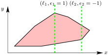
Figure 1.1: Weighted polygon $(\Delta,(\ell_{1},\,\ell_{2}),\,(1,\,-1))$.

(iv) the volume invariant: $m_{f}$ numbers measuring volumes of certain submanifolds at the singularities; (v) the twisting index invariant: $m_{f}$ integers measuring how twisted the system is around singularities. This is a subtle invariant, which depends on the representative chosen in (iii). Here, we write $m_{f}$ to emphasize that the singularities that $m_{f}$ counts are focus-focus singularities. We then proved that two semitoric systems $(M,\,\omega_{1},\,(J_{1},\,H_{1}))$ and $(M,\,\omega_{2},\,(J_{2},\,H_{2}))$ are isomorphic if and only if they have the same invariants (i)–(v), where an isomorphism is a symplectomorphism $\varphi\colon M_{1}\to M_{2}$ such that $\varphi^{*}(J_{2},\,H_{2})=(J_{1},\,f(J_{1},\,H_{1}))$ for some smooth function $f$.

We have found that some restrictions on these symplectic invariants must be imposed. Indeed, we call “semitoric list of ingredients” the following collection of items (i)-(v): (i) any integer number $0\leq m_{f}<\infty$; (ii) an $m_{f}$-tuple of real formal power series in two variables, with vanishing constant term and first terms $\sigma_{1}\,X+\sigma_{2}\,Y$ with $\sigma_{2}\in[0,\,2\,\pi)$; (iii) a Delzant weighted polygon $\Big{(}\Delta,\,(\ell_{j})_{j=1}^{m_{f}},\,(\epsilon_{j})_{j=1}^{m_{f}}\Big{)}$, of complexity $m_{f}$, where $\Delta$ is a polygon, the $\ell_{j}$ are again vertical lines intersecting $\Delta$ and the $\epsilon_{j}$ are $\pm 1$ signs giving each line $\ell_{j}$ an orientation; here the Delzant property for $\Delta$ is not the standard one for polygons, but rather a more delicate one for weighted polygons which takes into account the presence of the lines $\ell_{j}$; (iv) an $m_{f}$-tuple of positive real numbers $(h_{i})_{i=1}^{m_{f}}$ such that $0<h_{i}<\textup{length}(\Delta\cap\ell_{i})$ for each $i\in\{1,\ldots,m_{f}\}$. (v) an arbitrary collection of $m_{f}$ integers $(k_{i})_{i=1}^{m_{f}}$. Our main theorem (Theorem 4.6) says that, starting from a semitoric list of ingredients one can construct a $4$-dimensional semitoric integrable system $(M,\,\omega,\,(J,\,H))$ such that the list of its invariants is equal to this semitoric list. Moreover, $M$ is compact if and only the polygon in item (iii) is compact.

With this in mind we may formulate the uniqueness theorem in [17] as: two systems constructed in this fashion are isomorphic if and only if ingredients (i), (ii) and (iv) are identical for both systems and ingredients (iii) and (v) are related by some simple transformation. This is why, when we formulate the existence theorem, ingredients (iii) and (v) are given by orbits of respectively weighted polygons and pondered weighted polygons, under the action of certain groups. Together with [17, Th. 6.2], this gives the aforementioned classification (Theorem 4.7) .

While the construction of semitoric systems in the present paper is relatively self-contained, we are indebted to the articles of Delzant [6], Atiyah [1] and Guillemin-Sternberg [14], in the context of Hamiltonian torus actions, which served as an inspiration to study the more general situation of integrable systems with circular Hamiltonian symmetry. Furthermore, many works have played an important role in our investigation of $4$-dimensional semitoric systems, by serving as stepping stones to construct the symplectic invariants in [20] associated with semitoric systems; notably we used work of Dufour-Molino [8], Eliasson [9], Duistermaat [7], Miranda-Zung [16] and Vũ Ngọc [19],[20].

In this work, we are in a situation where the moment map $(J,H)$ is a “torus fibration” with singularities, and its base space becomes endowed with a singular integral affine structure. These structures have been studied in the context of integrable systems (in particular by Zung [23]), but also became a central concept in the works by Symington [18], Symington-Leung [15] in the context of symplectic geometry and topology, and by Gross-Siebert [10], [11], [12] and [13], among others, in the context of mirror symmetry and algebraic geometry. In fact, our ingredients (i), (iii) and (iv) could have been expressed in terms of this affine structure. However ingredients (ii) and (v) do not appear in the affine structure. Nevertheless it is expected that these ingredients play an important role in the quantum theory of integrable systems. We hope to be able to explore these ideas in the future.

The paper is structured as follows: in Section 2 we recall how to construct a collection of symplectic invariants for a semitoric system, and state more precisely that two semitoric systems are isomorphic precisely when they have the same invariants; this was done in [17], and we need to review it here in order to state the existence theorem for semitoric systems. In Section 3 we explain the symplectic glueing construction (i.e. how to glue symplectic manifolds equipped with momentum maps). The last two sections of the paper are respectively devoted to state the main theorem and to prove it. One might argue that the proof is more informative than the statement, as it gives an explicit construction of all semitoric integrable systems in dimension $4$.

Acknowledgements. We are grateful to Denis Auroux for offering many insightful comments, and for pointing out the papers of Gross and Siebert.

2 Review of the uniqueness theorem for semitoric systems

We recall the definition of the invariants that we assigned to a semitoric integrable system in our previous paper [17], to which we refer to further details. Then we state the uniqueness theorem proved therein.

2.1 Taylor series invariant

It was proven in [20] that a semitoric system $(M,\,\omega,\,F:=(J,\,H))$ has finitely many focus-focus critical values $c_{1},\,\dots,\,c_{m_{f}}$, that if we write $B:=F(M)$ then the set of regular values of $F$ is $\!\!\mathop{\rm~{}Int}\nolimits(B)\setminus\{c_{1},\dots,c_{m_{f}}\}$, that the boundary of $B$ consists of all images of elliptic singularities, and that the fibers of $F$ are connected. The integer $m_{f}$ was the first invariant that we associated with such a system. Let $i$ be an integer, with $1\leq i\leq m_{f}$.

We assume that the critical fiber $\mathcal{F}_{m}:=F^{-1}(c_{i})$ contains only one critical point $m$, which according to Zung [23] is a generic condition, and let $\mathcal{F}$ denote the associated singular foliation. Moreover, we will make for simplicity an even stronger generic assumption :

$$\begin{split}~{}&\text{If $m$ is a focus-focus critical point for }F,\\ &\text{then }m\text{ is the unique critical point of the level set }J^{-1}(J(m)).\end{split}$$

A semitoric system is simple if this genericity assumption is satisfied.

These conditions imply that the values $J(c_{1}),\,\dots,\,J(c_{m_{f}})$ are pairwise distinct. We assume throughout the article that the critical values $c_{i}$’s are ordered by their $J$-values : $J(c_{1})<J(c_{2})<\cdots<J(c_{m_{f}})$.

By Eliasson’s theorem [9] there exist symplectic coordinates $(x,\,y,\,\xi,\,\eta)$ in a neighborhood $U$ around $m$ in which $(q_{1},\,q_{2})$, given by

$$q_{1}=x\xi+y\eta,\,\,q_{2}=x\eta-y\xi,$$ (2.1)

is a momentum map for the foliation $\mathcal{F}$; here the critical point $m$ corresponds to coordinates $(0,\,0,\,0,\,0)$.

Fix $A^{\prime}\in\mathcal{F}_{m}\cap(U\setminus\{m\})$ and let $\Sigma$ denote a small 2-dimensional surface transversal to $\mathcal{F}$ at the point $A^{\prime}$, and let $\Omega$ be the open neighborhood of $\mathcal{F}_{m}$ which consists of the leaves which intersect the surface $\Sigma$. Since the Liouville foliation in a small neighborhood of $\Sigma$ is regular for both $F$ and $q=(q_{1},\,q_{2})$, there is a local diffeomorphism $\varphi$ of ${\mathbb{R}}^{2}$ such that $q=\varphi\circ{F}$, and we can define a global momentum map $\Phi=\varphi\circ{F}$ for the foliation, which agrees with $q$ on $U$. Write $\Phi:=(H_{1},\,H_{2})$ and $\Lambda_{z}:=\Phi^{-1}(z)$. Note that $\Lambda_{0}=\mathcal{F}_{m}.$ It follows from (2.1) that near $m$ the $H_{2}$-orbits must be periodic of primitive period $2\pi$ for any point in a (non-trivial) trajectory of $\mathcal{X}_{H_{1}}$.

Suppose that $A\in\Lambda_{z}$ for some regular value $z$. Let $\tau_{1}(z)>0$ be the time it takes the Hamiltonian flow associated with $H_{1}$ leaving from $A$ to meet the Hamiltonian flow associated with $H_{2}$ which passes through $A$, and let $\tau_{2}(z)\in{\mathbb{R}}/2\pi{\mathbb{Z}}$ the time that it takes to go from this intersection point back to $A$, hence closing the trajectory. Write $z=(z_{1},\,z_{2})=z_{1}+\!\!\mathop{\rm~{}i}\nolimits z_{2}$, and let $\!\!\mathop{\rm~{}ln}\nolimits z$ for a fixed determination of the logarithmic function on the complex plane. Let

$$\left\{\begin{array}[]{ccl}\sigma_{1}(z)&=&\tau_{1}(z)+\Re(\!\!\mathop{\rm~{}ln}\nolimits z)\\ \sigma_{2}(z)&=&\tau_{2}(z)-\Im(\!\!\mathop{\rm~{}ln}\nolimits z),\end{array}\right.$$ (2.2)

where $\Re$ and $\Im$ respectively stand for the real an imaginary parts of a complex number. Vũ Ngọc proved in [19, Prop. 3.1] that $\sigma_{1}$ and $\sigma_{2}$ extend to smooth and single-valued functions in a neighbourhood of $0$ and that the differential 1-form $\sigma:=\sigma_{1}\,\!\mathop{\rm d\!}\nolimits{}z_{1}+\sigma_{2}\,\!\mathop{\rm d\!}\nolimits{}z_{2}$ is closed. Notice that if follows from the smoothness of $\sigma_{2}$ that one may choose the lift of $\tau_{2}$ to ${\mathbb{R}}$ such that $\sigma_{2}(0)\in[0,\,2\pi)$. This is the convention used throughout. Following [19, Def. 3.1] , let $S_{i}$ be the unique smooth function defined around $0\in{\mathbb{R}}^{2}$ such that

$$\!\mathop{\rm d\!}\nolimits{}S_{i}=\sigma,\,\,\,\,S_{i}(0)=0$$ (2.3)

The Taylor expansion of $S_{i}$ at $(0,\,0)$ is denoted by $(S_{i})^{\infty}$.

Definition 2.1   The Taylor expansion $(S_{i})^{\infty}$ is a formal power series in two variables with vanishing constant term, and we say that $(S_{i})^{\infty}$ is the Taylor series invariant of $(M,\,\omega,\,(J,\,H))$ at the focus-focus point $c_{i}$. $\oslash$

2.2 Semitoric polygon invariant

The plane $\mathbb{R}^{2}$ is equipped with its standard affine structure with origin at $(0,0)$, and orientation. Let $\textup{Aff}(2,\mathbb{R}):=\textup{GL}(2,\mathbb{R})\ltimes\mathbb{R}^{2}$ be the group of affine transformations of $\mathbb{R}^{2}$. Let $\textup{Aff}(2,\mathbb{Z}):=\textup{GL}(2,\mathbb{Z})\ltimes\mathbb{R}^{2}$ be the subgroup of integral-affine transformations.

Let $\mathfrak{I}$ be the subgroup of $\!\!\mathop{\rm~{}Aff}\nolimits(2,\,{\mathbb{Z}})$ of those transformations which leave a vertical line invariant, or equivalently, an element of $\mathfrak{I}$ is a vertical translation composed with a matrix $T^{k}$, where $k\in{\mathbb{Z}}$ and

$$T^{k}:=\left(\begin{array}[]{cc}1&0\\ k&1\end{array}\right)\in\!\!\mathop{\rm~{}GL}\nolimits(2,\,{\mathbb{Z}}).$$ (2.6)

Let $\ell\subset{\mathbb{R}}^{2}$ be a vertical line in the plane, not necessarily through the origin, which splits it into two half-spaces, and let $n\in{\mathbb{Z}}$. Fix an origin in $\ell$. Let $t^{n}_{\ell}\colon{\mathbb{R}}^{2}\to{\mathbb{R}}^{2}$ be the identity on the left half-space, and $T^{n}$ on the right half-space. By definition $t^{n}_{\ell}$ is piecewise affine. Let $\ell_{i}$ be a vertical line through the focus-focus value $c_{i}=(x_{i},\,y_{i})$, where $1\leq i\leq m_{f}$, and for any tuple $\vec{n}:=(n_{1},\,\dots,\,n_{m_{f}})\in{\mathbb{Z}}^{m_{f}}$ we set $t_{\vec{n}}:=t^{n_{1}}_{\ell_{1}}\circ\,\cdots\,\circ t^{n_{m_{f}}}_{\ell_{m_{f}}}$. The map $t_{\vec{n}}$ is piecewise affine.

Definition 2.2   A rational convex polygon is the convex hull of a discrete set of points in $\mathbb{R}^{2}$, with the condition that each edge is directed along a vector with rational coefficients. $\oslash$

Let $B_{\!\!\mathop{\rm~{}r}\nolimits}:=\!\!\mathop{\rm~{}Int}\nolimits(B)\setminus\{c_{1},\,\ldots,\,c_{m_{f}}\}$, which is precisely the set of regular values of $F$. Given a sign $\epsilon_{i}\in\{-1,+1\}$, let $\ell_{i}^{\epsilon_{i}}\subset\ell_{i}$ be the vertical half line starting at $c_{i}$ at extending in the direction of $\epsilon_{i}$ : upwards if $\epsilon_{i}=1$, downwards if $\epsilon_{i}=-1$. Let $\ell^{\vec{\epsilon}}:=\bigcup_{i=1}^{m_{f}}\ell_{i}^{\epsilon_{i}}.$ In Th. 3.8 in [20] it was shown that for $\vec{\epsilon}\in\{-1,+1\}^{m_{f}}$ there exists a homeomorphism $f=f_{\epsilon}\colon B\to{\mathbb{R}}^{2}$, modulo a left composition by a transformation in $\mathfrak{I}$, such that $f|_{(B\setminus\ell^{\vec{\epsilon}})}$ is a diffeomorphism into its image $\Delta:=f(B)$, which is a rational convex polygon, $f|_{(B_{r}\setminus\ell^{\vec{\epsilon}})}$ is affine (it sends the integral affine structure of $B_{r}$ to the standard structure of ${\mathbb{R}}^{2}$) and $f$ preserves $J$: i.e.

$$f(x,\,y)=(x,\,f^{(2)}(x,\,y)).$$

$f$ satisfies further properties [17], which are relevant for the uniqueness proof. In order to arrive at $\Delta$ one cuts $(J,\,H)(M)\subset{\mathbb{R}}^{2}$ along each of the vertical half-lines $\ell_{i}^{\epsilon_{i}}$. Then the resulting image becomes simply connected and thus there exists a global 2-torus action on the preimage of this set. The polygon $\Delta$ is just the closure of the image of a toric momentum map corresponding to this torus action.

We can see that this polygon is not unique. The choice of the “cut direction” is encoded in the signs $\epsilon_{j}$, and there remains some freedom for choosing the toric momentum map. Precisely, the choices and the corresponding homeomorphisms $f$ are the following :

• an initial set of action variables $f_{0}$ of the form $(J,\,K)$ near a regular Liouville torus in [20, Step 2, pf. of Th. 3.8]. If we choose $f_{1}$ instead of $f_{0}$, we get a polygon $\Delta^{\prime}$ obtained by left composition with an element of $\mathfrak{I}$. Similarly, if we choose $f_{1}$ instead of $f_{0}$, we obtain $f$ composed on the left with an element of $\mathfrak{I}$;

• a tuple $\vec{\epsilon}$ of $1$ and $-1$. If we choose $\vec{\epsilon^{\prime}}$ instead of $\vec{\epsilon}$ we get $\Delta^{\prime}=t_{\vec{u}}(\Delta)$ with $u_{i}=(\epsilon_{i}-\epsilon^{\prime}_{i})/2$, by [20, Prop. 4.1, expr. (11)]. Similarly instead of $f$ we obtain $f^{\prime}=t_{\vec{u}}\circ f$.

Lemma 2.3.

Once $f_{0}$ and $\vec{\epsilon}$ have been fixed as in (a) and (b), respectively, then there exists a unique toric momentum map $\mu$ on $M_{r}:=F^{-1}(\textup{Int}{B}\setminus(\bigcup\ell_{j}^{\epsilon_{j}}))$ which preserves the foliation $\mathcal{F}$, and coincides with $f_{0}\circ F$ where they are both defined. Then, necessarily, the first component of $\mu$ is $J$, and we have

$$\overline{\mu(M_{r})}=\Delta.$$ (2.7)

Proof .  The uniqueness follows from the fact that $\textup{Int}{B}\setminus(\bigcup\ell_{j}^{\epsilon_{j}})$ is simply connected, and (2.7) follows directly from the construction of $\Delta$ in [20], since $\mu=f\circ F$. $\square$

We sometimes call $\mu$ the (generalized) momentum map associated with the polytope $\Delta$.

We need now for our purposes to formalize choices (a) and (b) in a single geometric object. Let $\!\!\mathop{\rm~{}Polyg}\nolimits({\mathbb{R}}^{2})$ be the space of rational convex polygons in ${\mathbb{R}}^{2}$. Let $\!\!\mathop{\rm~{}Vert}\nolimits({\mathbb{R}}^{2})$ be the set of vertical lines in ${\mathbb{R}}^{2}$. A weighted polygon of complexity $s$ is a triple of the form

$$\Delta_{\!\!\mathop{\mbox{\rm\scriptsize~{}w}}\nolimits}=\Big{(}\Delta,\,(\ell_{\lambda_{j}})_{j=1}^{s},\,(\epsilon_{j})_{j=1}^{s}\Big{)}$$

where $s$ is a non-negative integer, $\Delta\in\!\!\mathop{\rm~{}Polyg}\nolimits({\mathbb{R}}^{2})$, $\ell_{\lambda_{j}}\in\!\!\mathop{\rm~{}Vert}\nolimits({\mathbb{R}}^{2})$ for every $j\in\{1,\ldots,s\}$, and $\epsilon_{j}\in\{-1,\,1\}$ for every $j\in\{1,\ldots,s\}$,

$$\!\!\mathop{\rm~{}min}\nolimits_{s\in\Delta}\pi_{1}(s)<\lambda_{1}<\ldots<\lambda_{s}<\!\!\mathop{\rm~{}max}\nolimits_{s\in\Delta}\pi_{1}(s),$$

where $\pi_{1}\colon{\mathbb{R}}^{2}\to{\mathbb{R}}$ is the canonical projection $\pi_{1}(x,\,y)=x$ and $\pi_{1}(\ell_{\lambda_{j}})=\lambda_{j}$. For any $s\in{\mathbb{N}}$, let $G_{s}:=\{-1,\,+1\}^{s}$ and let $\mathcal{G}:=\{T^{k}\,\,|\,\,k\in{\mathbb{Z}}\}$. The group $\mathcal{G}$ acts naturally on $\mathbb{R}^{2}$ by the affine transformations $T^{k}$. Obviously, it sends a rational convex polygon to a rational convex polygon. It corresponds to the transformation described in (a). On the other hand, the transformation described in (b) can be encoded by the group $G_{s}$ acting on the triple $\Delta_{\!\!\mathop{\mbox{\rm\scriptsize~{}w}}\nolimits}$ by the formula

$$(\epsilon^{\prime}_{j})_{j=1}^{s}\cdot\Big{(}\Delta,\,(\ell_{\lambda_{j}})_{j=1}^{s},\,(\epsilon_{j})_{j=1}^{s}\Big{)}=\Big{(}t_{\vec{u}}(\Delta),\,(\ell_{\lambda_{j}})_{j=1}^{s},\,(\epsilon^{\prime}_{j}\,\epsilon_{j})_{j=1}^{s}\Big{)},$$ (2.8)

where $\vec{u}=((\epsilon_{i}-\epsilon^{\prime}_{i})/2)_{i=1}^{s}$. This, however, does not always preserve the convexity of $\Delta$, as is easily seen when $\Delta$ is the unit square centered at the origin and $\lambda_{1}=0$. However, when $\Delta$ comes from the construction described above for a semitoric system $(J,H)$, the convexity is preserved. Thus, we say that

Definition 2.4   A weighted polygon is admissible when the $G_{s}$-action preserves convexity. We denote by $\mathcal{W}\!\!\mathop{\rm~{}Polyg}\nolimits_{s}({\mathbb{R}}^{2})$ the space of all admissible weighted polygons of complexity $s$. $\oslash$

The set $G_{s}\times\mathcal{G}$ is an abelian group, with the natural product action. The action of $G_{s}\times\mathcal{G}$ on $\mathcal{W}\!\!\mathop{\rm~{}Polyg}\nolimits_{s}({\mathbb{R}}^{2})$, is given by:

$$((\epsilon^{\prime}_{j})_{j=1}^{s},\,T^{k})\cdot\Big{(}\Delta,\,(\ell_{\lambda_{j}})_{j=1}^{s},\,(\epsilon_{j})_{j=1}^{s}\Big{)}=\Big{(}t_{\vec{u}}(T^{k}(\Delta)),\,(\ell_{\lambda_{j}})_{j=1}^{s},\,(\epsilon^{\prime}_{j}\,\epsilon_{j})_{j=1}^{s}\Big{)},$$

where $\vec{u}=((\epsilon_{i}-\epsilon^{\prime}_{i})/2)_{i=1}^{s}$.

Definition 2.5   We call a semitoric polygon the equivalence class of an admissible weighted polygon under the $(G_{m_{f}}\times\mathcal{G})$-action. $\oslash$

Let $\Delta$ be a rational convex polygon obtained from the momentum image $(J,\,H)(M)$ according to the above construction of cutting along the vertical half-lines $\ell_{1}^{\epsilon_{1}},\ldots,\ell_{m_{f}}^{\epsilon_{m_{f}}}$.

Definition 2.6   The semitoric polygon invariant of $(M,\,\omega,\,(J,\,H))$ is the semitoric polygon equal to the $(G_{m_{f}}\times\mathcal{G})$-orbit

$$(G_{m_{f}}\times\mathcal{G})\cdot\Big{(}\Delta,\,(\ell_{j})_{j=1}^{m_{f}},\,(\epsilon_{j})_{j=1}^{m_{f}}\Big{)}\in\mathcal{W}\!\!\mathop{\rm~{}Polyg}\nolimits_{m_{f}}({\mathbb{R}}^{2})/(G_{m_{f}}\times\mathcal{G}).$$ (2.9)

$\oslash$

2.3 The Volume Invariant

Consider a focus-focus critical point $m_{i}$ whose image by $(J,\,H)$ is $c_{i}$, and let $\Delta$ be a rational convex polygon corresponding to the system $(M,\,\omega,\,(J,\,H))$. If $\mu$ is a toric momentum map for the system $(M,\,\omega,\,(J,\,H))$ corresponding to $\Delta$, then the image $\mu(m_{i})$ is a point in the interior of $\Delta$, along the line $\ell_{i}$. We proved in [17] that the vertical distance

$$h_{i}:=\mu(m_{i})-\min_{s\in\ell_{i}\cap\Delta}\pi_{2}(s)>0$$ (2.10)

is independent of the choice of momentum map $\mu$. Here $\pi_{2}\colon{\mathbb{R}}^{2}\to{\mathbb{R}}$ is $\pi_{2}(x,\,y)=y$. The reasoning behind writing the word “volume” in the name of this invariant is that it has the following geometric interpretation: the singular manifold $Y_{i}=J^{-1}(c_{i})$ splits into $Y_{i}\cap\{H>H(m_{i})\}$ and $Y_{i}\cap\{H<H(m_{i})\}$, and $h_{i}$ is the Liouville volume of $Y_{i}\cap\{H<H(m_{i})\}$.

2.4 The Twisting-Index Invariant

The twisting-index expresses the fact that there is, in a neighbourhood of any focus-focus point $c_{i}$, a privileged toric momentum map $\nu$. This momentum map, in turn, is due to the existence of a unique hyperbolic radial vector field in a neighbourhood of the focus-focus fiber. Therefore, one can view the twisting-index as a dynamical invariant. Since any semitoric polygon defines a (generalized) toric momentum map $\mu$, we will be able to define the twisting-index as the integer $k_{i}\in\mathbb{Z}$ such that

$$\!\mathop{\rm d\!}\nolimits\mu=T^{k_{i}}\!\mathop{\rm d\!}\nolimits\nu.$$

We could have defined equivalently the twisting-indices by comparing the privileged momentum maps at different focus-focus points.

The precise definition of $k_{i}$ requires some care, which we explain now.

Let $\Delta_{\!\!\mathop{\mbox{\rm\scriptsize~{}w}}\nolimits}=\Big{(}\Delta,\,(\ell_{j})_{j=1}^{m_{f}},\,(\epsilon_{j})_{j=1}^{m_{f}}\Big{)}$ be as in expression (2.9). Let $\ell:=\ell_{i}^{\epsilon_{i}}\subset{\mathbb{R}}^{2}$ be the vertical half-line starting at $c_{i}$ and pointing in the direction of $\epsilon_{i}\,e_{2}$, where $e_{1},\,e_{2}$ are the canonical basis vectors of $\mathbb{R}^{2}$. By Eliasson’s theorem, there is a neighbourhood $W=W_{i}$ of the focus-focus critical point $m_{i}=F^{-1}(c_{i})$, a local symplectomorphism $\phi:({\mathbb{R}}^{4},\,0)\to W$, and a local diffeomorphism $g$ of $({\mathbb{R}}^{2},\,0)$ such that $F\circ\phi=g\circ q$, where $q$ is given by (2.1). Since $q_{2}\circ\phi^{-1}$ has a $2\pi$-periodic Hamiltonian flow, it is equal to $J$ in $W$, up to a sign. Composing if necessary $\phi$ by $(x,\xi)\mapsto(-x,-\xi)$ one can assume that $q_{2}=J\circ\phi$ in $W$, i.e. $g$ is of the form $g(q_{1},\,q_{2})=(q_{2},\,g_{2}(q_{1},\,q_{2}))$. Upon composing $\phi$ by $(x,\,y,\,\xi,\,\eta)\mapsto(-\xi,\,-\eta,\,x,\,y)$, which changes $(q_{1},\,q_{2})$ into $(-q_{1},\,q_{2})$, one can assume that $\frac{\partial g_{2}}{\partial q_{1}}(0)>0$. In particular, near the origin $\ell$ is transformed by $g^{-1}$ into the positive real axis if $\epsilon_{i}=1$, or the negative real axis if $\epsilon_{i}=-1$.

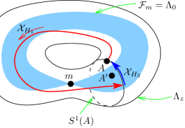
Figure 2.1: Singular foliation near the leaf $\mathcal{F}_{m}$, where $S^{1}(A)$ denotes the $S^{1}$-orbit generated by $H_{2}$.

Let us now fix the origin of angular polar coordinates in ${\mathbb{R}}^{2}$ on the positive real axis, let $V=F(W)$ and define $\tilde{F}=(H_{1},\,H_{2})=g^{-1}\circ F$ on $F^{-1}(V)$ (notice that $H_{2}=J$). Recall that near any regular torus there exists a Hamiltonian vector field $\mathcal{X}_{p}$, whose flow is $2\pi$-periodic, defined by

$$2\pi\mathcal{X}_{p}=(\tau_{1}\circ\tilde{F})\mathcal{X}_{H_{1}}+(\tau_{2}\circ\tilde{F})\mathcal{X}_{J},$$

where $\tau_{1}$ and $\tau_{2}$ are functions on ${\mathbb{R}}^{2}\setminus\{0\}$ satisfying (2.2), with $\sigma_{1}(0)>0$. In fact $\tau_{2}$ is multivalued, but we determine it completely in polar coordinates with angle in $[0,\,2\pi)$ by requiring continuity in the angle variable and $\sigma_{2}(0)\in[0,\,2\pi)$. In case $\epsilon_{i}=1$, this defines $\mathcal{X}_{p}$ as a smooth vector field on $F^{-1}(V\setminus\ell)$. In case $\epsilon_{i}=-1$ we keep the same $\tau_{2}$-value on the negative real axis, but extend it by continuity in the angular interval $[\pi,\,3\pi)$. In this way $\mathcal{X}_{p}$ is again a smooth vector field on $F^{-1}(V\setminus\ell)$. Let $\mu$ be the generalized toric momentum map associated to $\Delta$. On $F^{-1}(V\setminus\ell$), $\mu$ is smooth, and its components $(\mu_{1},\,\mu_{2})=(J,\,\mu_{2})$ are smooth Hamiltonians, whose vector fields $(\mathcal{X}_{J},\mathcal{X}_{\mu_{2}})$ are tangent to the foliation, have a $2\pi$-periodic flow, and are a.e. independent. Since the couple $(\mathcal{X}_{J},\mathcal{X}_{p})$ shares the same properties, there must be a matrix $A\in\textup{GL}(2,{\mathbb{Z}})$ such that $(\mathcal{X}_{J},\mathcal{X}_{\mu_{2}})=A(\mathcal{X}_{J},\mathcal{X}_{p})$. This is equivalent to saying that there exists an integer $k_{i}\in{\mathbb{Z}}$ such that

$$\mathcal{X}_{\mu_{2}}=k_{i}\mathcal{X}_{J}+\mathcal{X}_{p}.$$

It was shown in [17, Prop. 5.4] that $k_{i}$ is well defined, i.e. does not depend on choices. The integer $k_{i}$ is called the twisting index of $\Delta_{\!\!\mathop{\mbox{\rm\scriptsize~{}w}}\nolimits}$ at the focus-focus critical value $c_{i}$. It was shown in [17, Lem. 5.6] that there exists a unique smooth function $H_{p}$ on $F^{-1}(V\setminus\ell)$ the Hamiltonian vector field of which is $\mathcal{X}_{p}$ and such that $\lim_{m\to m_{i}}H_{p}=0.$ The toric momentum map $\nu:=(J,\,H_{p})$ is called the privileged momentum map for $(J,\,H)$ around the focus-focus value $c_{i}$. If $k_{i}$ is the twisting index of $c_{i}$, one has $\!\mathop{\rm d\!}\nolimits\mu=T^{k_{i}}\!\mathop{\rm d\!}\nolimits\nu$ on $F^{-1}(V)$. However, the twisting index does depend on the polygon $\Delta$. Thus, since we want to define an invariant of the initial semitoric system, we need to take into account the actions of $G_{s}$ and $\mathcal{G}$.

If we transform the polygon $\Delta$ by a global affine transformation in $T^{r}\in\mathcal{G}$ this has no effect on the privileged momentum map $\nu$, whereas it changes $\mu$ into $T^{r}\mu$. From this characterization it follows that all the twisting indices $k_{i}$ are replaced by $k_{i}+r$. It was shown in [17, Prop. 5.8] that if two weighted polygons $\Delta_{\!\!\mathop{\mbox{\rm\scriptsize~{}w}}\nolimits}$ and $\Delta^{\prime}_{\!\!\mathop{\mbox{\rm\scriptsize~{}weight}}\nolimits}$ lie in the same $G_{m_{f}}$-orbit, then the twisting indices $k_{i},\,k^{\prime}_{i}$ associated to $\Delta_{\!\!\mathop{\mbox{\rm\scriptsize~{}w}}\nolimits}$ and $\Delta^{\prime}_{\!\!\mathop{\mbox{\rm\scriptsize~{}weight}}\nolimits}$ at their respective focus-focus critical values $c_{i},\,c^{\prime}_{i}$ are equal.

For any integer $s$, consider the action of the product $G_{s}\times\mathcal{G}$ on the space $\mathcal{W}\!\!\mathop{\rm~{}Polyg}\nolimits_{s}({\mathbb{R}}^{2})\times{\mathbb{Z}}^{s}$:

$$((\epsilon^{\prime}_{j})_{j=1}^{s}),\,T^{k})\star\Big{(}\Delta,\,(\ell_{\lambda_{j}})_{j=1}^{s},\,(\epsilon_{j})_{j=1}^{s},\,(k_{j})_{j=1}^{s}\Big{)}=\Big{(}t_{\vec{u}}(T^{k}(\Delta)),\,(\ell_{\lambda_{j}})_{j=1}^{s},\,(\epsilon^{\prime}_{j}\,\epsilon_{j})_{j=1}^{s},\,(k_{j}+k)_{j=1}^{s}\Big{)}$$

where $\vec{u}=((\epsilon_{j}-\epsilon^{\prime}_{j})/2)_{j=1}^{s}$, for all integer $j$, with $j\in\{1,\,\ldots,\,s\}$.

Definition 2.7   The twisting-index invariant of $(M,\,\omega,\,(J,\,H))$ is the $(G_{m_{f}}\times\mathcal{G})$-orbit of weighted polygon pondered by twisting indices at the focus-focus singularities of the system given by

$$(G_{m_{f}}\times\mathcal{G})\star\Big{(}\Delta,\,(\ell_{j})_{j=1}^{m_{f}},\,(\epsilon_{j})_{j=1}^{m_{f}},\,(k_{j})_{j=1}^{m_{f}}\Big{)}\in(\mathcal{W}\!\!\mathop{\rm~{}Polyg}\nolimits_{m_{f}}({\mathbb{R}}^{2})\times{\mathbb{Z}}^{m_{f}})/(G_{m_{f}}\times\mathcal{G}).$$ (2.11)

$\oslash$

2.5 Uniqueness theorem

To a semitoric system we assign the above list of invariants and state the main theorem in [17].

Definition 2.8   Let $(M,\,\omega,\,(J,\,H))$ be a $4$-dimensional simple semitoric integrable system. The list of invariants of $(M,\,\omega,\,(J,\,H))$ consists of the following items.

• The integer number $0\leq m_{f}<\infty$ of focus-focus singular points.

• The $m_{f}$-tuple $((S_{i})^{\infty})_{i=1}^{m_{f}}$, where $(S_{i})^{\infty}$ is the Taylor series of the $i^{\!\!\mathop{\mbox{\rm\scriptsize~{}th}}\nolimits}$ focus-focus point.

• The semitoric polygon invariant, c.f. Definition 2.3.

• The volume invariant, i.e. the $m_{f}$-tuple $(h_{i})_{i=1}^{m_{f}}$, where $h_{i}$ is the height of the $i^{\!\!\mathop{\mbox{\rm\scriptsize~{}th}}\nolimits}$ focus-focus point.

• The twisting-index invariant, c.f. Definition 2.1.

$\oslash$

Theorem 2.9 (Th. 6.2, [17]).

The two $4$-dimensional simple semitoric integrable systems $(M_{1},\,\omega_{1},(J_{1},\,H_{1}))$ and $(M_{2},\,\omega_{2},(J_{2},\,H_{2}))$ are isomorphic if and only if the list of invariants (i)-(v), as in Definition 2.5, of $(M_{1},\,\omega_{1},(J_{1},\,H_{1}))$ is equal to the list of invariants (i)-(v) of $(M_{2},\,\omega_{2},(J_{2},\,H_{2}))$.

3 The symplectic glueing construction

In this section we explain how to symplectically glue an arbitrary collection of symplectic manifolds $(M_{\alpha})_{\alpha\in A}$ equipped with continuous, proper maps $F_{\alpha}\colon M_{\alpha}\to\mathbb{R}$ to form a new symplectic manifold $M$ equipped with a continuous, proper map which restricted to $M_{\alpha}$ is equal to $F_{\alpha}$, c.f. Theorem 3.10. The results of this section, while perhaps well-known among experts, we could not find in the literature.

3.1 Glueing maps, glueing groupoid

Let $A$ be an arbitrary set of indices, and let $(M_{\alpha})_{\alpha\in A}$ be a family of sets. Recall that the disjoint union of the sets $M_{\alpha}$, $\alpha\in A$ is the subset of $(\bigcup_{\alpha\in A}M_{\alpha})\times A$ defined by

$$\bigsqcup_{\alpha\in A}M_{\alpha}:=\{(x,\,\alpha)\,|\,x\in M_{\alpha}\}.$$

We denote by $j_{\alpha}$, $\alpha\in A$, the natural inclusions : $j_{\alpha}:~{}M_{\alpha}\hookrightarrow\bigsqcup_{\alpha\in A}M_{\alpha},\,\,x\mapsto(x,\,\alpha)$. Notice that if $B\subset A$ then $\bigsqcup_{\alpha\in B}M_{\alpha}\subset\bigsqcup_{\alpha\in A}M_{\alpha}$. Of course, if all $M_{\alpha}$’s are pairwise disjoint, as sets, then there is a natural bijection bewteen $\bigsqcup_{\alpha\in A}M_{\alpha}$ and the usual union $\bigcup_{\alpha\in A}M_{\alpha}$.

If the $M_{\alpha}$’s are topological spaces, the disjoint union $\bigsqcup_{\alpha\in A}M_{\alpha}$ is endowed with the final topology : the finest topology that makes the inclusions $j_{\alpha}$ continuous. In particular $j_{\alpha}(M_{\alpha})$ is an open set in $\bigsqcup_{\alpha\in A}M_{\alpha}$.

Definition 3.1   A glueing map for the family $(M_{\alpha})_{\alpha\in A}$ is a homeomorphism $\varphi:U_{\alpha}\rightarrow U_{\beta}$ where $(\alpha,\beta)\in A^{2}$, and $U_{\alpha}\subset M_{\alpha}$ and $U_{\beta}\subset M_{\beta}$ are open sets. $\oslash$

In this text we use the standard set-theoretical convention that the notation $\varphi$ includes the source and target sets $U_{\alpha}$ and $U_{\beta}$; in particular the notation $\varphi(x)$ implies $x\in U_{\alpha}$. When required, we use the notation $U_{\varphi}^{s}$ and $U_{\varphi}^{t}$ for the source and target sets of $\varphi$ (assuming $U_{\varphi}^{t}=\varphi(U_{\varphi}^{s})$).

Definition 3.2   Let $\mathcal{G}$ be a collection of glueing maps for $(M_{\alpha})_{\alpha\in A}$. The associated glueing groupoid $G$ is the groupoid generated by the set of all restrictions of all glueing maps $\varphi\in\mathcal{G}$ to open subsets of the source sets, with the natural groupoid law : $\varphi_{2}\circ\varphi_{1}$ exists whenever the image of the source set of $\varphi_{1}$ is included in the source set of $\varphi_{2}$. $\oslash$

Definition 3.3   We say that $\mathcal{G}$ is free when there is no nontrivial $\varphi\in G$ with both source and target in the same set $M_{\alpha}$. $\oslash$

3.2 Topological glueing

We define now the general patching construction. Throughout this section, and unless otherwise stated, we do not require topological spaces to be paracompact or Hausdorff.

Definition 3.4   Let $(M_{\alpha})_{\alpha\in A}$ be a collection of pairwise disjoint topological spaces, and $G$ an associated glueing groupoid. From this we define the set $M$, called the glueing of $(M_{\alpha})_{\alpha\in A}$ along $G$, as $M:=\bigsqcup_{\alpha\in A}M_{\alpha}/\sim$ where $\sim$ is the equivalence relation on $\bigsqcup_{\alpha\in A}M_{\alpha}$ defined by

$$(x,\,\alpha)\sim(x^{\prime},\beta)\Longleftrightarrow\left(x=x^{\prime}\,\text{ or there exists }\,\varphi\in G\,\,\textup{with}\,\,x^{\prime}=\varphi(x)\right).$$

$\oslash$

Let us check that $\sim$ is indeed an equivalence relation. The reflexivity is obvious. If $(x,\,\alpha)\sim(x^{\prime},\,\beta)$ and $(x,\,\alpha)\neq(x^{\prime},\,\beta)$ then $\varphi(x)=x^{\prime}$ for some $\varphi\in G$. But $G$ is a groupoid so $\varphi^{-1}\in G$ and of course $x=\varphi^{-1}(x^{\prime})$, so $(x^{\prime},\,\beta)\sim(x,\,\alpha)$, which proves the symmetry property. Finally, if $(x,\,\alpha)\sim(x^{\prime},\,\beta)$ and $(x^{\prime},\,\beta)\sim(x^{\prime\prime},\,\gamma)$ then there exist $\varphi$ anf $\varphi^{\prime}$ in $G$ such that $\varphi(x)=x^{\prime}$ and $\varphi^{\prime}(x^{\prime})=x^{\prime\prime}$. Therefore $\varphi^{\prime}\circ\varphi$ is well-defined on an open neighbourhood of $x$, so $\varphi^{\prime}\circ\varphi\in G$, and $(x,\,\alpha)\sim(x^{\prime\prime},\,\gamma)$, so we have shown the transitivity property.

Here again we could have dropped the assumption that the $M_{\alpha}$’s are pairwise disjoint, or we could have used a standard union instead of a disjoint union.

The following lemma follows from the definition of the equivalence relation.

Lemma 3.5.

Let $\pi:\bigsqcup_{\alpha\in A}M_{\alpha}\rightarrow M$ be the quotient map. For any subset $K\subset M_{\alpha}$, one has

$$\pi^{-1}(y_{\alpha}(K))=j_{\alpha}(K)\cup\left(\bigcup_{\varphi\in G}j_{\alpha(\varphi)}(\varphi(K\cap U_{\varphi}^{s}))\right),$$

where it is assumed that the union is over all $\varphi$ whose source set $U_{\varphi}^{s}$ intersects $K$, and $\alpha(\varphi)$ is the element in $A$ such that $U_{\varphi}^{t}\subset M_{\alpha(\varphi)}$.

Lemma 3.6.

For the natural quotient topology on $M$, the maps $y_{\alpha}=\pi\circ j_{\alpha}:M_{\alpha}\rightarrow M$, $\alpha\in A$ are open and continuous. They are injective if and only if $\mathcal{G}$ is free.

Proof.

By definition of the quotient topology, the map $\pi$ is continuous. Hence $y_{\alpha}=\pi\circ j_{\alpha}$ is continuous. Finally if $U\subset M_{\alpha}$ is open, then if follows from Lemma 3.5 that $\pi^{-1}(y_{\alpha}(U))$ is open in $\bigsqcup_{\alpha\in A}M_{\alpha}$. This means that $y_{\alpha}(U)$ is open in $M$.

Fix $\alpha\in A$. Let $x$ and $x^{\prime}$ be elements of $M_{\alpha}$. If $y_{\alpha}(x)=y_{\alpha}(x^{\prime})$ then either $x=x^{\prime}$ or $\varphi(x)=x^{\prime}$ for some $\varphi\in G$. The latter is ruled out by the assumption that there is no nontrivial $\varphi\in G$ with both source and target in $M_{\alpha}$. Thus in this case $y_{\alpha}$ is injective. If the condition is violated then there exist $x\neq x^{\prime}$ in $M_{\alpha}$ with $j_{\alpha}(x)\sim j_{\alpha}(x^{\prime})$ so $y_{\alpha}$ cannot be injective. ∎

3.3 Smooth glueing

Lemma 3.7.

If all $M_{\alpha}$’s are smooth manifolds, all $\varphi\in\mathcal{G}$ are diffeomorphisms and $\mathcal{G}$ is free then there exists a unique smooth structure on $M$ for which the maps $y_{\alpha}$, $\alpha\in A$ are embeddings.

Proof.

Let $U\subset M_{\alpha}$ be open and let $g:U\rightarrow\mathbb{R}^{n}$ be a homeomorphism. By Lemma 3.6, $y_{\alpha}$ is a homeomorphism onto its image. Let $\tilde{U}=y_{\alpha}(U)$ and $\tilde{g}=g\circ((y_{\alpha})|_{U})^{-1}$. Then $\tilde{U}$ is an open subset of $M$ and $\tilde{g}:\tilde{U}\rightarrow\mathbb{R}^{n}$ is a homeomorphism. This shows that any chart of $M_{\alpha}$ descends onto a chart of $M$. Obviously the union of a family of open covers of $M_{\alpha}$ for all $\alpha\in A$ descends to an open cover of $M$. In order to get an atlas on $M$, it remains to check the compatibility condition when an open set $\tilde{V}_{\alpha}$ coming from an atlas of $M_{\alpha}$ intersects an open set $\tilde{V}_{\beta}$ coming from an atlas of $M_{\beta}$. Thus, let $(V_{\alpha},g_{\alpha})$, $V_{\alpha}\subset M_{\alpha}$ and $(V_{\beta},g_{\beta})$, $V_{\beta}\subset M_{\beta}$ be local charts such that $y_{\alpha}(V_{\alpha})=y_{\beta}(V_{\beta})$ and $\alpha\neq\beta$. Now consider the formula, given by Lemma 3.5 :

$$j_{\alpha}(V_{\alpha})\cup\left(\bigcup_{\varphi\in G}j_{\alpha(\varphi)}(\varphi(V_{\alpha}\cap U_{\varphi}^{s}))\right)=j_{\beta}(V_{\beta})\cup\left(\bigcup_{\varphi\in G}j_{\alpha(\varphi)}(\varphi(V_{\beta}\cap U_{\varphi}^{s}))\right).$$

Because $\mathcal{G}$ is free, any $\varphi$ whose source set intersects $V_{\alpha}$ and with $\alpha(\varphi)=\alpha$ must be the identity. Hence, in the lefthand side one can ommit all $\varphi$’s such that $\alpha(\varphi)=\alpha$. For the same reason, one can assume that all $\alpha(\varphi)$’s are pairwise different. Of course the analogue observation holds for the righthand side. Hence we can equate terms in the unions (up to permutation). In particular there must exist some $\varphi$ with $\alpha(\varphi)=\beta$ and $j_{\beta}(\varphi(V_{\alpha}\cap U_{\varphi}^{s}))=j_{\beta}(V_{\beta}).$ Since $j_{\beta}$ is injective, $\varphi(V_{\alpha}\cap U_{\varphi}^{s})=V_{\beta}$. Let $x\in V_{\beta}$ and $x^{\prime}=\varphi^{-1}(x)\in V_{\alpha}$. Then $y_{\alpha}(x^{\prime})=y_{\beta}(x)$, i.e. $x^{\prime}=y_{\alpha}^{-1}\circ y_{\beta}(x)$. Thus $((y_{\alpha})|_{V_{\alpha}})^{-1}\circ(y_{\beta})|_{V_{\beta}}=(\varphi^{-1})|_{V_{\beta}}.$ Hence the transition map for the charts $\tilde{g}_{u}:=g_{u}\circ((y_{u})|_{V_{u}})^{-1}$ ($u=\alpha,\beta$) is equal to

$$\tilde{g}_{\alpha}\circ{\tilde{g}_{\beta}}^{-1}=g_{\alpha}\circ\left(((y_{\alpha})|_{V_{\alpha}})^{-1}\circ(y_{\beta})|_{V_{\beta}}\right)\circ g_{\beta}^{-1}=g_{\alpha}\circ\varphi^{-1}\circ g_{\beta}^{-1},$$ (3.1)

which is indeed a composition of local diffeomorphisms. Thus $M$ has a natural smooth structure.

Consider now the map $y_{\alpha}:M_{\alpha}\hookrightarrow M$. Read in a chart $(\tilde{V}_{\alpha},\tilde{g}_{\alpha})$ of $M$, with $\tilde{g}_{\alpha}:=g_{\alpha}\circ((y_{\alpha})|_{V_{\alpha}})^{-1}$, for some chart $(V_{\alpha},g_{\alpha})$ on $M_{\alpha}$, it becomes $\tilde{g}_{\alpha}\circ y_{\alpha}=(g_{\alpha})|_{V_{\alpha}},$ which is a local diffeomorphism. Since we already know that $y_{\alpha}$ is a homeomorphism onto its image, it is an embedding.

Conversely, if $y_{\alpha}$, $\alpha\in A$ have to be embeddings for some smooth structure on $M$, then any local chart on $M_{\alpha}$ is sent by $y_{\alpha}$ to a local chart on $M$. Thus, necessarily, we obtain the same charts on $M$ as the ones we’ve just constructed. ∎

Remark 3.7   The smooth manifold $M$ given in Lemma 3.7 is not necessarily a Hausdorff space. The definition of manifold in Bourbaki [3] does not require $M$ to be a Hausdorff topological space, or a paracomact space. These are, however, conditions most frequently required. It follows from Bourbaki [3] that $M$ is Hausdorff if, and only if, for any two smooth charts $\varphi\colon U\subset M\to{\mathbb{R}}^{n}$, $\psi\colon V\subset M\to{\mathbb{R}}^{n}$ constructed as in the proof of Lemma 3.7, we have that the graph of $\psi\circ\varphi^{-1}\colon\varphi(U\cap V)\to\psi(U\cap V)$ is closed in $\varphi(U)\times\psi(V)\subset{\mathbb{R}}^{n}\times{\mathbb{R}}^{n}$. $\oslash$

3.4 Symplectic glueing

Unlike in the previous two sections, we shall be assuming that the $M_{\alpha}$, $\alpha\in A$, are Haudorff, paracompact smooth manifolds. Moreover, we will be assuming that there exist continuous, proper maps $F_{\alpha}\colon M\to{\mathbb{R}}^{n}$ which can be glued together to give rise to a proper map $F\colon M\to{\mathbb{R}}$. With the aid of $F$ we will show that the Hausdorff and paracompactness properties of the $M_{\alpha}$ are inherited by $M$.

Lemma 3.8.

If for each $\alpha\in A$, $M_{\alpha}$ is symplectic with symplectic form $\omega_{\alpha}$, and if all $\varphi\in\mathcal{G}$ are symplectomorphisms (and $\mathcal{G}$ is free) then there exists a unique symplectic structure $\omega$ on $M$ such that $y_{\alpha}^{*}\omega=\omega_{i},\quad\alpha\in A$.

Proof.

Because (1) all $y_{\alpha}$’s are embeddings, (2) $\bigcup_{\alpha\in A}y_{\alpha}(M_{\alpha})=M$, (3) when $y_{\alpha}(M_{\alpha})$ intersects $y_{\beta}(M_{\beta})$, $\alpha\neq\beta$, then $y_{\beta}^{-1}\circ(y_{\alpha})=\varphi$ for some $\varphi\in G$ with $\varphi^{*}\omega_{\beta}=\omega_{\alpha}$, the formula $y_{\alpha}^{*}\omega=\omega_{\alpha}$ defines a unique symplectic form $\omega$ on $M$. ∎

We can finally apply this technique in our case :

Proposition 3.9.

Let $(M_{\alpha})_{\alpha\in A}$ be a collection of symplectic manifolds, each equipped with a map $F_{\alpha}:M_{\alpha}\rightarrow\mathbb{R}^{n}$. For any $\alpha,\beta\in A$ let $D_{\alpha\beta}:=F_{\alpha}(M_{\alpha})\cap F_{\beta}(M_{\beta})$ and assume

1. $U_{\alpha}:=F_{\alpha}^{-1}(D_{\alpha\beta})$ and $U_{\beta}:=F_{\beta}^{-1}(D_{\alpha\beta})$ are open.

2. $\varphi_{\alpha\beta}:U_{\alpha}\rightarrow U_{\beta}$ is a symplectomorphism such that $\varphi_{\alpha\beta}^{*}F_{\beta}=F_{\alpha}$.

3. When $D_{\alpha\beta\gamma}:=F_{\alpha}(M_{\alpha})\cap F_{\beta}(M_{\beta})\cap F_{\gamma}(M_{\gamma})\neq\varnothing$, $\varphi_{\beta\gamma}\circ\varphi_{\alpha\beta}=\varphi_{\alpha\gamma}\,\text{(restricted to }F_{\alpha}^{-1}(D_{\alpha\beta\gamma})\text{)}.$

Then the smooth manifold $M$ obtained by glueing the collection $(M_{\alpha})_{\alpha\in A}$ along the set of all $(\varphi_{\alpha\beta})$ is symplectic, and there exists a unique map $F:M\rightarrow\mathbb{R}^{n}$ verifying $F_{\alpha}=F\circ y_{\alpha}$, where $y_{\alpha}:M_{\alpha}\hookrightarrow M$, $\alpha\in A$ are the natural symplectic embeddings.

Proof.

The third assumption (cocycle condition) implies that the corresponding glueing groupoid is free. ∎

Theorem 3.10 (Symplectic Glueing).

Let $(M_{\alpha})_{\alpha\in A}$ be a collection of symplectic manifolds, each equipped with a continuous, proper map $F_{\alpha}:M_{\alpha}\rightarrow V_{\alpha}\subset\mathbb{R}^{n}$, where $V_{\alpha}$ is open. For any $\alpha,\beta\in A$ let $D_{\alpha\beta}:=V_{\alpha}\cap V_{\beta}$ and assume

1. $\varphi_{\alpha\beta}:F_{\alpha}^{-1}(D_{\alpha\beta})\rightarrow F_{\beta}^{-1}(D_{\alpha\beta})$ is a symplectomorphism such that $\varphi_{\alpha\beta}^{*}F_{\beta}=F_{\alpha}$.

2. When $V_{\alpha}\cap V_{\beta}\cap V_{\gamma}\neq\varnothing$, $\varphi_{\beta\gamma}\circ\varphi_{\alpha\beta}=\varphi_{\alpha\gamma}$.

Then the smooth manifold $M$ obtained by glueing the collection $(M_{\alpha})_{\alpha\in A}$ along the set of all $(\varphi_{\alpha\beta})$ is Hausdorff, paracompact (in other words, a smooth manifold in the usual sense) and symplectic, and there exists a unique continuous, proper map $F:M\rightarrow\bigcup_{\alpha\in A}V_{\alpha}\subset\mathbb{R}^{n}$ verifying $F_{\alpha}=F\circ y_{\alpha}$, where $y_{\alpha}:M_{\alpha}\hookrightarrow M$, $\alpha\in A$, are the natural symplectic embeddings.

Proof.

The main statement is a corollary of Proposition 3.9 since $F^{-1}(V_{\alpha}\cap V_{\beta})=F^{-1}(F(M_{\alpha})\cap F(M_{\beta}))$ and thus the right handside is automatically open.

Next we show that $M$ is Hausdorff. Let $\bar{z},\,\bar{w}\in M$, where $z,\,w\in\bigsqcup_{\alpha\in A}M_{\alpha}$. There are two possibilities, that $F(\bar{z})=F(\bar{w})$ or that $F(\bar{z})\neq F(\bar{w})$. If $F(\bar{z})=F(\bar{w})$, then by definition of $F$ (i.e. $F_{\alpha}=F\circ y_{\alpha}$), there exists $\alpha\in A$ such that $z\in M_{\alpha}$ and $w\in M_{\alpha}$. Here we are viewing $M_{\alpha}$ as a subset of $\bigsqcup_{\alpha\in A}M_{\alpha}$, under the canonical identification $y_{\alpha}$. Because $M_{\alpha}$ is Hausdorff, there exist open sets $U_{z}\subset M_{\alpha}$, $U_{w}\subset M_{\alpha}$, with $z\in U_{z}$, $w\in U_{w}$ and $U_{z}\cap U_{w}=\varnothing$. Because $M_{\alpha}$ is open in $\bigsqcup_{\alpha\in A}M_{\alpha}$, by Lemma 3.6 we have that $\pi(U_{z})$ and $\pi(U_{w})$ are open subsets of $M$. By construction, $\bar{z}\in\pi(U_{z})$, $\bar{w}\in\pi(U_{w})$. It follows from the definition of $\pi$ as the quotient map $\bigsqcup_{\alpha\in A}M_{\alpha}\to M=\bigsqcup_{\alpha\in A}M_{\alpha}/\sim$, that $\pi(U_{z})\cap\pi(U_{w})=\pi(U_{z}\cap U_{w})=\pi(\varnothing)=\varnothing$.

Suppose on the other hand that $F(\bar{z})\neq F(\bar{w})$. Since $F(\bar{z})\in{\mathbb{R}}^{n}$, $F(\bar{w})\in{\mathbb{R}}^{n}$, and ${\mathbb{R}}^{n}$ is Hausdorff, there exist open sets $W_{z}$ and $W_{w}$ in ${\mathbb{R}}^{n}$ such that $F(\bar{z})\in W_{z}$, $F(\bar{w})\in W_{w}$ and $W_{z}\cap W_{w}=\varnothing$. Since $F$ is continuous, $F^{-1}(W_{z})$ and $F^{-1}(W_{w})$ are open. Also, by construction, $\bar{z}\in F^{-1}(W_{z})$ and $\bar{w}\in F^{-1}(W_{w})$. Of course $F^{-1}(W_{z})\cap F^{-1}(W_{w})=F^{-1}(W_{z}\cap W_{w})=\varnothing$.

Let us show that $F$ is proper. Let $V:=\bigcup_{\alpha\in A}V_{\alpha}$. Let $K\subset V$ be compact in $V$. Since $K$ is compact, there exists a finite number of open balls $B_{i}$ of radius $\epsilon>0$ that cover $K$ and such that any $\overline{B_{i}}$ is included in some $V_{\alpha(i)}$, $\alpha(i)\in A$. Let $\{O_{\beta}\}_{\beta\in B}$ be an open cover of $F^{-1}(K)$. For any $i$, the set $\overline{B_{i}}$ is compact in $V_{\alpha(i)}$; hence $F_{\alpha}^{-1}(\overline{B_{i}})$ is compact in $M_{\alpha}$. Thus $y_{\alpha}(F_{\alpha}^{-1}(\overline{B_{i}}))$ is compact in $M$, and hence there exists a finite subset $B_{i}\subset B$ such that $\bigcup_{\beta\in B_{i}}O_{\beta}\supset y_{\alpha}(F_{\alpha}^{-1}(\overline{B_{i}})).$ We can conclude, using the fact that

$$\textup{for all}\,\,U\subset V_{\alpha},\quad y_{\alpha}(F_{\alpha}^{-1}(U))=F^{-1}(U),$$ (3.2)

that $F^{-1}(K)\subset\bigcup_{i}\bigcup_{\beta\in B_{i}}O_{\beta},$ which shows that $F^{-1}(K)$ is indeed compact.

To complete the properness proof we must show that equality (3.2) holds. Indeed, the inclusion of sets $y_{\alpha}(F_{\alpha}^{-1}(U))\subset F^{-1}(U)$ follows directly from the equality $F\circ y_{\alpha}=F_{\alpha}$. For the converse, we come back to the definition of $M$. If $\bar{z}\in F^{-1}(U)$ there must exist some $z_{\beta}\in M_{\beta}$ such that $\pi(z_{\beta})=\bar{z}$ ($\pi$ is the quotient map of Lemma 3.5). Thus $F_{\beta}(z_{\beta})=F(\bar{z})$. This means that $V_{\alpha}\cap V_{\beta}$ is not empty, and there is a symplectomorphism $\varphi_{\beta\alpha}$ such that $z_{\alpha}:=\varphi_{\beta\alpha}(z_{\beta})\in M_{\alpha}$. This implies $\pi(z_{\alpha})=\pi(z_{\beta})=\bar{z}$. Thus $F(\bar{z})=F_{\alpha}(z_{\alpha})$ which proves the inclusion $F^{-1}(U)\subset y_{\alpha}(F_{\alpha}^{-1}(U)).$

We have left to show that $M$ is a paracompact space. We have previously shown that $F\colon M\to V$ is a proper map, so in particular, the fibers of $F$ are compact. On the other hand, for each $\alpha\in A$, $M_{\alpha}$ is a manifold in the usual sense, and hence it is locally compact, which then implies that $\bigsqcup_{\alpha\in A}M_{\alpha}$ is locally compact. We claim that $M$ is locally compact. Indeed, let $\bar{z}\in M$, where $z\in M_{\alpha}$ for some $\alpha$. Because $M_{\alpha}$ is locally compact, there is a compact neighborhood $K_{z}$ of $z$ in $M_{\alpha}$ containing an open set $U_{z}$, with $z\in U_{z}$. Since $\pi$ is continuous, $\pi(K_{z})$ is compact. Since $\pi$ is open, $\pi(U_{z})$ is open, and hence $\pi(K_{z})$ is a compact neighborhood of $\bar{z}$, and we have shown that $M$ is locally compact.

On the other hand, a continuous, proper map between locally compact Hausdorff spaces is closed see [5, Prop. 3, p. 16]. We have already shown that $M$ is Hausdorff and locally compact. Hence, since $F\colon M\to V$ is a proper map, it is a also a closed map.

Next we deduce the paracompactness of $M$ from the following result [21, 20G, p. 153], [4, Th. 1]: if $f\colon X\to Y$ is a continuous, closed surjective mapping between topological spaces with compact fibers, and $Y$ is paracompact, then $X$ is paracompact as well. We can apply this result with $X$ equal to $M$, $Y$ equal to $F(M)\subset{\mathbb{R}}^{n}$, and $f$ equal to $F\colon M\to F(M)$. The map $F\colon M\to F(M)$ is continuous, closed, and it has compact fibers, and $F(M)$, as a subset of $\mathbb{R}^{n}$, is paracompact. Hence $M$ is paracompact. This concludes the proof of the proposition. ∎

4 Main Theorem: statement

Again we equip the plane $\mathbb{R}^{2}$ with its standard affine structure with origin at $(0,0)$, and orientation.

4.1 Delzant semitoric polygons

Let $\Delta\in\!\!\mathop{\rm~{}Polyg}\nolimits({\mathbb{R}}^{2})$ be a convex rational polygon in $\mathbb{R}^{2}$, as in Definition 2.2. Recall that in our terminology, $\Delta$ is not necessarily compact. We call a vertex a point in the boundary $\partial\Delta$ where the meeting edges are not colinear. We shall make the following assumption

• The intersection of $\Delta$ with a vertical line is either compact or empty.

Consider such a vertical line intersecting the polytope. If the intersection is not just a point, then it is a vertical segment. The top end of this segment is said to belong to the top-boundary of $\Delta$.

To each vertex $z$ of $\Delta$ we associate a couple $\mathcal{B}_{z}$ of primitive integral vectors starting at $z$ and extending along the direction of the edges meeting at $z$, in the order that makes them oriented. Then $\mathcal{B}_{z}$ defines a $\mathbb{Z}$-basis of $\mathbb{Z}^{2}\subset\mathbb{R}^{2}$ when, viewed as a $2\times 2$ matrix, its determinant is equal to $1$.

Let $s\in\mathbb{N}^{*}$ and let $(\lambda_{1},\dots,\lambda_{s})\in\mathbb{R}^{s}$ with $\lambda_{1}<\cdots<\lambda_{s}$. As before $\ell_{\lambda_{j}}$ is the vertical line $\{x=\lambda_{j}\}$. We are interested only in the following case

• The vertical lines $\ell_{\lambda_{j}}$, $j=1,\dots,s$ intersect the top-boundary of $\Delta$.

Let $T$ be the linear transformation acting as the matrix

$$T:=T^{1}=\begin{pmatrix}1&0\\ 1&1\end{pmatrix}.$$

Definition 4.1   Let $z$ be a vertex of the polygon $\Delta$ and $(u,\,v)=\mathcal{B}_{z}$. The point $z$ is called

• a Delzant corner when there is no vertical line $\ell_{\lambda_{j}}$ through it and $\det(u,\,v)=1$,

• a hidden Delzant corner when there is a vertical line $\ell_{\lambda_{j}}$ through it, it belongs to the top-boundary, and $\det(u,\,Tv)=1$.

• a fake corner when there is a vertical line $\ell_{\lambda_{j}}$ through it, it belongs to the top-boundary, and $\det(u,\,Tv)=0$.

$\oslash$

For the following lemma recall the definition of admissible weighted polygon, c.f. Definition 2.3.

Lemma 4.2.

Let $\Delta$ be a convex rational polygon equipped with a set of vertical lines $(\ell_{\lambda_{1}},\dots,\ell_{\lambda_{s}})$, such that the assumptions (a1) and (a2) are satisfied. Suppose moreover that

• any point in the top-boundary that belongs to some vertical line $\ell_{\lambda_{j}}$ is either a hidden Delzant corner or a fake corner;

• any other vertex of $\Delta$ is a Delzant corner.

Then the triple

$$\left(\Delta,(\ell_{\lambda_{j}})_{j=1}^{s},(1,\dots,1)\right)$$

is an admissible weighted polygon.

Proof.

We need to show that the convexity is preserved under the $G_{s}$-action. This amounts to show that for any $j=1,\dots,s$, the polygon $t_{\vec{e_{j}}}(\Delta)$ is convex, where $(\vec{e_{1}},\,\dots,\,\vec{e_{s}})$ is the canonical basis of $\mathbb{Z}^{s}$. Since $t_{\vec{e_{j}}}$ is affine on both half-spaces delimited by the vertical line $\ell_{\lambda_{j}}$, it suffices to show that $t_{\vec{e_{j}}}(\Delta)$ is locally convex near the points where $\ell_{\lambda_{j}}$ meets the boundary $\partial\Delta$.

We let $\{a,z\}=\ell_{\lambda_{j}}\cap\partial\Delta$ and assume $z$ lies on the top boundary. By assumption, $z$ is either a hidden Delzant corner or a fake corner. Let us consider the vectors $(u,\,v)=\mathcal{B}_{z}$. Because $z$ belongs to the top-boundary, the vector $u$ must be directed to the lefthand side of $z$ and $v$ to the righthand side. Since the transformation $t_{\vec{e_{j}}}$ acts only on the right half-space (and there it acts as $T$), the transformed edges of $t_{\vec{e_{j}}}(\Delta)$ at $z$ are directed along $(u,\,Tv)$. By assumption $\det(u,\,Tv)$ is either $0$ or $1$, which implies local convexity at $z$.

Now consider the “bottom boundary” at the point $a$. By assumption the polygon is already locally convex at $a$ (which means $\det(u,v)\geqslant 0$), and a quick calculation shows that the action of $t_{\vec{e_{j}}}$ may only make it even “more” convex. ∎

It is easy to see that the properties of the lemma are preserved by the $\mathcal{G}$-action. Thus we can state the following definition.

Definition 4.3   Let $[\Delta_{\!\!\mathop{\mbox{\rm\scriptsize~{}w}}\nolimits}]$ be a semitoric polygon as in Definition 2.3, and suppose that $\Delta_{\!\!\mathop{\mbox{\rm\scriptsize~{}w}}\nolimits}$ is a representative of the form $\Big{(}\Delta,\,(\ell_{\lambda_{j}})_{j=1}^{s},\,(\epsilon_{j})_{j=1}^{s}\Big{)}$ with all $\epsilon_{j}$’s equal to $+1$. Then $[\Delta_{\!\!\mathop{\mbox{\rm\scriptsize~{}w}}\nolimits}]$ is called a Delzant semitoric polygon (of complexity $s$) if the polygon $\Delta$ equipped with the vertical lines $\ell_{\lambda_{j}}$ satisfies the hypothesis of Lemma 4.2. $\oslash$

We denote by $\mathcal{D}\textup{Polyg}_{s}({\mathbb{R}}^{2})\subset\mathcal{W}\textup{Polyg}_{s}({\mathbb{R}}^{2})/G_{s}\times\mathcal{G}$ the space of Delzant semitoric polygons of complexity $s$, where $s<\infty$.

The following observation is a consequence of the construction of the homeomorphism $f$ in Section 2.2.

Lemma 4.4.

The semitoric polygon in item (iii) of Definition 2.5 is a Delzant semitoric polygon.

In addition, note also that for any representative $\Delta$ of the semitoric polygon $[\Delta_{\!\!\mathop{\mbox{\rm\scriptsize~{}w}}\nolimits}]$ in Definition 2.5, and for each $i\in\{1,\ldots,\,m_{f}\}$ as in item (iv) of Definition 2.5, the height $h_{i}$ satisfies the inequality

$$0<h_{i}<\textup{length}(\Delta\cap\ell_{i}).$$ (4.1)

This is because by (2.10) we have $h_{i}:=\mu(m_{i})-\min_{s\in\ell_{i}\cap\Delta}\pi_{2}(s)$, where $\mu$ is a toric momentum map for the system $(M,\,\omega,\,(J,\,H))$ corresponding to $\Delta$. Now, since $\mu(m_{i})$ is a point in the interior of $\Delta$, along the line $\ell_{i}$, expression (4.1) follows.

4.2 Main Theorem

The following definition describes a collection of abstract ingredients. As we will see in the theorem following the definition, each such a list of elements determines one, and one only one, integrable system on a symplectic $4$-manifold (which is not necessarily a compact manifold, but we can characterize precisely when it is in terms of one of the ingredients of the list). Moreover, this integrable system is of semitoric type.

In the definition the term ${\mathbb{R}}[[X,\,Y]]$ refers to the algebra of real formal power series in two variables, and ${\mathbb{R}}[[X,\,Y]]_{0}$ is the subspace of such series with vanishing constant term, and first term $\sigma_{1}\,X+\sigma_{2}\,Y$ with $\sigma_{2}\in[0,\,2\,\pi)$.

Definition 4.5   A semitoric list of ingredients consists of the following items.

• An integer number $0\leq m_{f}<\infty$.

• An $m_{f}$-tuple of Taylor series $((S_{i})^{\infty})_{i=1}^{m_{f}}\in({\mathbb{R}}[[X,\,Y]]_{0})^{m_{f}}$.

• A Delzant semitoric polygon $[\Delta_{\!\!\mathop{\mbox{\rm\scriptsize~{}w}}\nolimits}]$ of complexity $m_{f}$, as in Definition 4.2.

  We denote the representative $\Delta_{\!\!\mathop{\mbox{\rm\scriptsize~{}w}}\nolimits}$ of $[\Delta_{\!\!\mathop{\mbox{\rm\scriptsize~{}w}}\nolimits}]$ by $\Big{(}\Delta,\,(\ell_{\lambda_{j}})_{j=1}^{m_{f}},\,(\epsilon_{j})_{j=1}^{m_{f}}\Big{)}$.

• An $m_{f}$-tuple of numbers $(h_{j})_{j=1}^{m_{f}}$ such that $0<h_{j}<\textup{length}(\Delta\cap\ell_{i})$ for each $j\in\{1,\ldots,m_{f}\}$.

• A $(G_{m_{f}}\times\mathcal{G})$-orbit of $(\Delta_{\!\!\mathop{\mbox{\rm\scriptsize~{}w}}\nolimits},(k_{j})_{j=1}^{m_{f}})$, where $(k_{j})_{j=1}^{m_{f}}$ is a collection of integers.

$\oslash$

Now we are ready to state the main theorem, the proof of which is contructive and, in view of Section 2 and Lemma 4.4, gives a recipe to construct all semitoric integrable systems up to isomorphisms.

Theorem 4.6.

For each semitoric list of ingredients, as in Definition 4.2, there exists a $4$-dimensional simple semitoric integrable system $(M,\,\omega,\,(J,\,H))$, such that the list of invariants (i)-(v) of $(M,\,\omega,\,(J,\,H))$ as in Definition 2.5 is equal to this list of ingredients. Moreover, $M$ is compact if and only the polygon in (iii) is compact.

4.3 Classification of $4$-dimensional semitoric systems

Consequently, putting Theorem 4.6 together with Theorem 2.9 proved in [17], we obtain the classification of integrable systems in symplectic $4$-manifolds.

Theorem 4.7 (Classification of $4$-dimensional semitoric integrable systems).

For each semitoric list of ingredients, as in Definition 4.2, there exists a $4$-dimensional simple semitoric integrable system with list of invariants equal to this list of ingredients, c.f. Definition 2.5. Moreover, two $4$-dimensional simple semitoric integrable systems are isomorphic if, and only if, they are constructed from the same list of ingredients.

5 Proof of Main Theorem

Let $\Big{(}\Delta,\,(\ell_{\lambda_{j}})_{j=1}^{s},\,(\epsilon_{j})_{j=1}^{s}\Big{)}$ be a representative of $[\Delta_{\!\!\mathop{\mbox{\rm\scriptsize~{}w}}\nolimits}]$ with all $\epsilon_{j}$’s equal to $+1$. The strategy is to use the glueing procedure of Section 3 in order to obtain a semitoric system by constructing a suitable singular torus fibration above $\Delta\subset\mathbb{R}^{2}$.

For $j=1,\dots,m_{f}$, let $c_{j}\in\mathbb{R}^{2}$ be the point with coordinates

$$c_{j}=(\lambda_{j},\,h_{j}+\min(\pi_{2}(\Delta\cap\ell_{\lambda_{j}}))).$$ (5.1)

Because of the assumption on $h_{j}$, all points $c_{j}$ lie in the interior of the polygon $\Delta$. We call these points nodes. We denote by $\ell_{j}^{+}$ the vertical half-line through $c_{j}$ pointing upwards. We call these half-lines cuts.

We have divided the proof of the theorem in a preliminary step, three intermediate steps and a conclusive step. In the preliminary step we construct a convenient covering of the polygon $\Delta$.

Then we proceed as follows. First we construct a “semitoric system” over the part of the polygon away from the sets in the covering that contain the cuts $\ell_{j}^{+}$; then we attach to this “semitoric system” the focus-focus fibrations i.e. the models for the systems in a small neighborhood of the nodes. Third, we continue to glue the local models in a small neighborhood of the cuts. The “semitoric system” is given by a proper toric map only in the preimage of the polygon away from the cuts. We use the results of Section 3 as a stepping stone throughout.

Finally we recover the smoothness of the system and observe that the invariants of the system are precisely the ingredients we started with.

Preliminary stage. A convenient covering.—

We construct an open cover of the polygon. Because of the discreteness of the set of vertices of the polygon, and the local compactness of $\mathbb{R}^{2}$, we one can find an open cover $(\Omega_{\alpha})_{\alpha\in A}$ of $\Delta$ such that the following three properties hold: there exists $\rho>0$ such that all $\Omega_{\alpha}$’s are integral-affine images of the open cube $C:=I^{2}$ with $I=:]-\rho,\rho[$, i.e for every $\alpha\in A$ there exists $R_{\alpha}\in\textup{Aff}(2,\mathbb{Z})$, such that $\Omega_{\alpha}=R_{\alpha}(C)$; each vertex of the polygon, and each node, is contained in only one open set $\Omega_{\alpha}$; two open sets containing a vertex or a node never intersect each other. In fact, if

$$C_{\!\!\mathop{\mbox{\rm\scriptsize~{}e}}\nolimits}:=C\cap\{y\geqslant 0\},\,\,\,\,\,C_{\!\!\mathop{\mbox{\rm\scriptsize~{}ee}}\nolimits}:=C\cap\{x\geqslant 0\}\cap\{y\geqslant 0\},$$

one can assume that, for any $\alpha\in A$, (1) if $\Omega_{\alpha}$ intersects $\partial\Delta$ but does not contain any vertex then $\Omega_{\alpha}\cap\Delta=R_{\alpha}(C_{\!\!\mathop{\mbox{\rm\scriptsize~{}e}}\nolimits})$, and that (2) if $\Omega{{}_{\alpha}}$ contains a Delzant corner, then $\Omega_{\alpha}\cap\Delta=R_{\alpha}(C_{\!\!\mathop{\mbox{\rm\scriptsize~{}ee}}\nolimits})$. The first case holds since along any edge one can find a primitive vector, and complete it to a $\mathbb{Z}$-basis of $\mathbb{Z}^{2}$. It remains to compose by a suitable translation to position the image of $C_{\!\!\mathop{\mbox{\rm\scriptsize~{}e}}\nolimits}$ at the right place. The second case is similar, since at a Delzant corner the primitive vectors of the meeting edges form a $\mathbb{Z}$-basis of $\mathbb{Z}^{2}$, c.f. Definition 4.1.

First stage. Away from the cuts.—

Let $A^{\prime}\subset A$ be the subset obtained by removing all indices intersecting the cuts. We construct a semitoric system above $\bigcup_{\alpha\in A^{\prime}}\Omega_{\alpha}$, by glueing the following local models. Let ${\mathbb{D}}$ be the open disk in $\!\!\mathop{\rm~{}T}\nolimits^{*}\mathbb{R}=\mathbb{R}^{2}$ of radius $\sqrt{2\rho}$, centered at the origin. Consider the following models: the regular model : $M_{\!\!\mathop{\mbox{\rm\scriptsize~{}r}}\nolimits}:={\mathbb{T}}^{2}\times C\subset T^{*}{\mathbb{T}}^{2}$ with momentum map

$$F_{\!\!\mathop{\mbox{\rm\scriptsize~{}r}}\nolimits}(x_{1},\,x_{2},\,\xi_{1},\,\xi_{2}):=(\xi_{1},\,\xi_{2});$$

the tranversally elliptic model : $M_{\!\!\mathop{\mbox{\rm\scriptsize~{}e}}\nolimits}:=({\mathbb{T}}^{1}\times I)\times{\mathbb{D}}\subset\!\!\mathop{\rm~{}T}\nolimits^{*}{\mathbb{T}}^{1}\times\!\!\mathop{\rm~{}T}\nolimits^{*}\mathbb{R}$, with momentum map

$$F_{\!\!\mathop{\mbox{\rm\scriptsize~{}e}}\nolimits}(x_{1},\,\xi_{1},\,x_{2},\,\xi_{2}):=(\xi_{1},\,(x_{2}^{2}+\xi_{2}^{2})/2);$$

and the elliptic-elliptic model : $M_{\!\!\mathop{\mbox{\rm\scriptsize~{}ee}}\nolimits}:={\mathbb{D}}\times{\mathbb{D}}\subset\!\!\mathop{\rm~{}T}\nolimits^{*}\mathbb{R}\times\!\!\mathop{\rm~{}T}\nolimits^{*}\mathbb{R}$, with momentum map

$$F_{\!\!\mathop{\mbox{\rm\scriptsize~{}ee}}\nolimits}(x_{1},\,\xi_{1},\,x_{2},\,\xi_{2}):=((x_{1}^{2}+\xi_{1}^{2})/2,\,(x_{2}^{2}+\xi_{2}^{2})/2).$$

Observe that $F_{\!\!\mathop{\mbox{\rm\scriptsize~{}r}}\nolimits}(M_{\!\!\mathop{\mbox{\rm\scriptsize~{}r}}\nolimits})=C$, $F_{\!\!\mathop{\mbox{\rm\scriptsize~{}e}}\nolimits}(M_{\!\!\mathop{\mbox{\rm\scriptsize~{}e}}\nolimits})=C_{\!\!\mathop{\mbox{\rm\scriptsize~{}e}}\nolimits}$, and $F_{\!\!\mathop{\mbox{\rm\scriptsize~{}ee}}\nolimits}(M_{\!\!\mathop{\mbox{\rm\scriptsize~{}ee}}\nolimits})=C_{\!\!\mathop{\mbox{\rm\scriptsize~{}ee}}\nolimits}$. Notice also that these models are all toric, in the sense that the momentum maps generate an effective hamiltonian ${\mathbb{T}}^{2}$ action. What’s more, these momentum maps are proper for the topology induced on their images.

Given any $\Omega_{\alpha}$, $\alpha\in A^{\prime}$, we obtain a (singular) Lagrangian momentum map over $\Omega_{\alpha}$, whose image is precisely $\Omega_{\alpha}\cap\Delta$ by the following simple rule : (a) If $\Omega_{\alpha}$ contains no boundary points of $\Delta$ and no nodes, then we choose $M_{\alpha}:=M_{\!\!\mathop{\mbox{\rm\scriptsize~{}r}}\nolimits}$, with momentum map $F_{\alpha}:=R_{\alpha}\circ F_{\!\!\mathop{\mbox{\rm\scriptsize~{}r}}\nolimits}$; (b) If $\Omega_{\alpha}$ interects $\partial\Delta$ but does not contain vertices, we choose $M_{\alpha}:=M_{\!\!\mathop{\mbox{\rm\scriptsize~{}e}}\nolimits}$, with momentum map $F_{\alpha}:=R_{\alpha}\circ F_{\!\!\mathop{\mbox{\rm\scriptsize~{}e}}\nolimits}$. (c) If $\Omega_{\alpha}$ contains a Delzant coner, we choose $M_{\alpha}:=M_{\!\!\mathop{\mbox{\rm\scriptsize~{}ee}}\nolimits}$, with momentum map $F_{\alpha}:=R_{\alpha}\circ F_{\!\!\mathop{\mbox{\rm\scriptsize~{}ee}}\nolimits}$.

We describe now the transition functions : when $\Delta_{\alpha\beta}:=\Omega_{\alpha}\cap\Omega_{\beta}\neq\varnothing$, we want to define a symplectomorphism

$$\varphi_{\alpha\beta}:F_{\alpha}^{-1}(\Delta_{\alpha\beta})\rightarrow F_{\beta}^{-1}(\Delta_{\alpha\beta})\,\,\,\,\,\,\,\textup{such that}\,\,\,\,\varphi_{\alpha\beta}^{*}F_{\beta}=F_{\alpha}.$$ (5.2)

For this we use the following notation : when $R\in\textup{Aff}(2,\,\mathbb{Z})$, we denote by $\tilde{R}$ the symplectomorphism $\tilde{R}:{\mathbb{T}}^{2}\times\mathbb{R}^{2}(=\!\!\mathop{\rm~{}T}\nolimits^{*}{\mathbb{T}}^{2})\to{\mathbb{T}}^{2}\times\mathbb{R}^{2}$ given by $(x,\,\xi)\mapsto((\raisebox{2.58334pt}{${\scriptstyle t}$}\!\!\mathop{\rm~{}d}\nolimits\!R)^{-1}x,\,R\xi)$, where $\!\!\mathop{\rm~{}d}\nolimits\!R$ is the linear part of $R$. Remark that $\xi\circ\tilde{R}=R\circ\xi$.

Case 1. If both $F_{\alpha}$ and $F_{\beta}$ are regular models, we let

$$\varphi_{\alpha\beta}:=\tilde{R}_{\beta}^{-1}\,\tilde{R}_{\alpha}.$$ (5.3)

Then $F_{\beta}\circ\varphi_{\alpha\beta}=R_{\beta}\circ F_{\!\!\mathop{\mbox{\rm\scriptsize~{}r}}\nolimits}\circ\varphi_{\alpha\beta}=F_{\!\!\mathop{\mbox{\rm\scriptsize~{}r}}\nolimits}\circ\tilde{R}_{\beta}\circ\varphi_{\alpha\beta}=F_{\!\!\mathop{\mbox{\rm\scriptsize~{}r}}\nolimits}\circ\tilde{R}_{\alpha}=F_{\alpha}$, i.e. (5.2) holds.

Case 2. If $F_{\alpha}$ is regular and $F_{\beta}$ is transversally elliptic, we introduce the symplectomorphism (symplectic polar coordinates)

$$\begin{split}\varphi_{\!\!\mathop{\mbox{\rm\scriptsize~{}re}}\nolimits}:M_{\!\!\mathop{\mbox{\rm\scriptsize~{}r}}\nolimits}\cap({\mathbb{T}}^{1}\times\mathbb{R})\times({\mathbb{T}}^{1}\times\mathbb{R}_{+}^{*})&\rightarrow({\mathbb{T}}^{1}\times\mathbb{R})\times(\mathbb{R}^{2}\setminus\{0\})\cap M_{\!\!\mathop{\mbox{\rm\scriptsize~{}e}}\nolimits}\\ (x_{1},\,\xi_{1},\,x_{2},\,\xi_{2})&\mapsto(x_{1},\,\xi_{1},\,\sqrt{2\,\xi_{2}}\cos(x_{2}),\,-\sqrt{2\,\xi_{2}}\sin(x_{2})).\end{split}$$

Notice that $\varphi_{\!\!\mathop{\mbox{\rm\scriptsize~{}re}}\nolimits}^{*}F_{\!\!\mathop{\mbox{\rm\scriptsize~{}e}}\nolimits}=F_{\!\!\mathop{\mbox{\rm\scriptsize~{}r}}\nolimits}$. Thus we can define

$$\varphi_{\alpha\beta}:=\varphi_{\!\!\mathop{\mbox{\rm\scriptsize~{}re}}\nolimits}\circ\tilde{R}_{\beta}^{-1}\tilde{R}_{\alpha}.$$ (5.4)

We have $F_{\beta}\circ\varphi_{\alpha\beta}=R_{\beta}\circ F_{\!\!\mathop{\mbox{\rm\scriptsize~{}e}}\nolimits}\circ\varphi_{\!\!\mathop{\mbox{\rm\scriptsize~{}re}}\nolimits}\circ\tilde{R}_{\beta}^{-1}\tilde{R}_{\alpha}=R_{\beta}\circ F_{\!\!\mathop{\mbox{\rm\scriptsize~{}r}}\nolimits}\circ\tilde{R}_{\beta}^{-1}\tilde{R}_{\alpha}=F_{\!\!\mathop{\mbox{\rm\scriptsize~{}r}}\nolimits}\circ\tilde{R}_{\alpha}=F_{\alpha}$, i.e. (5.2) holds.

Case 3. Similarly, if $F_{\alpha}$ is regular and $F_{\beta}$ is elliptic-elliptic, we introduce the symplectomorphism

$$\begin{split}\varphi_{\!\!\mathop{\mbox{\rm\scriptsize~{}ree}}\nolimits}:M_{\!\!\mathop{\mbox{\rm\scriptsize~{}r}}\nolimits}\cap({\mathbb{T}}^{1}\times\mathbb{R}_{+}^{*})\times({\mathbb{T}}^{1}\times\mathbb{R}_{+}^{*})&\rightarrow(\mathbb{R}^{2}\setminus\{0\})\times(\mathbb{R}^{2}\setminus\{0\})\cap M_{\!\!\mathop{\mbox{\rm\scriptsize~{}ee}}\nolimits}\\ (x_{1},\,\xi_{1},\,x_{2},\,\xi_{2})&\mapsto\left(\begin{split}\sqrt{2\,\xi_{1}}\cos(x_{1}),\,&-\sqrt{2\,\xi_{1}}\sin(x_{1}),\,\\ \sqrt{2\,\xi_{2}}\cos(x_{2}),\,&-\sqrt{2\,\xi_{2}}\sin(x_{2}).\end{split}\right)\end{split}$$

Again $\varphi_{\!\!\mathop{\mbox{\rm\scriptsize~{}ree}}\nolimits}^{*}F_{\!\!\mathop{\mbox{\rm\scriptsize~{}ee}}\nolimits}=F_{\!\!\mathop{\mbox{\rm\scriptsize~{}r}}\nolimits}$, and if we define

$$\varphi_{\alpha\beta}:=\varphi_{\!\!\mathop{\mbox{\rm\scriptsize~{}ree}}\nolimits}\circ\tilde{R}_{\beta}^{-1}\,\tilde{R}_{\alpha},$$ (5.5)

(5.2) holds.

Case 4. If both $F_{\alpha}$ and $F_{\beta}$ are transversally elliptic models, then the affine map $R_{\alpha\beta}:=R_{\beta}^{-1}R_{\alpha}$ is an oriented transformation that preserves the upper half-plane. Thus the horizontal axis is globally preserved, and the vector $e_{1}=(1,\,0)$ is an eigenvector of $\!\!\mathop{\rm~{}d}\nolimits\!R_{\alpha\beta}$. Since $\!\!\mathop{\rm~{}d}\nolimits\!R_{\alpha\beta}\in\textup{SL}(2,\,\mathbb{Z})$, it is of the form

$$T_{k}:=\begin{pmatrix}1&k\\ 0&1\end{pmatrix}$$

for some $k\in\mathbb{Z}$. Hence $R_{\alpha\beta}=\tau_{u}\circ T_{k}$ where $\tau_{u}$ is the translation by a horizontal vector $u=(u_{1},\,0)$. Consider the symplectomorphism $\bar{R}_{\alpha\beta}(x_{1},\,\xi_{1},\,x_{2},\,\xi_{2}):=(x_{1}^{\prime},\,\xi_{1}^{\prime},\,\,x_{2}^{\prime},\,\xi_{2}^{\prime})$ of $\!\!\mathop{\rm~{}T}\nolimits^{*}{\mathbb{T}}^{1}\times\!\!\mathop{\rm~{}T}\nolimits^{*}\mathbb{R}$ given by

$$\left\{\begin{aligned} x_{1}^{\prime}&=x_{1}\\ \xi_{1}^{\prime}&=\xi_{1}+k(x_{2}^{2}+\xi_{2}^{2})/2+u_{1}\\ (x_{2}^{\prime}+\!\!\mathop{\rm~{}i}\nolimits\,\xi_{2}^{\prime})&=\textup{e}^{\!\!\mathop{\rm~{}i}\nolimits\,kx_{1}}(x_{2}+i\xi_{2}).\end{aligned}\right.$$

Observe that $F_{\!\!\mathop{\mbox{\rm\scriptsize~{}e}}\nolimits}\circ\bar{R}_{\alpha\beta}=R_{\alpha\beta}\circ F_{\!\!\mathop{\mbox{\rm\scriptsize~{}e}}\nolimits}$. Now we define

$$\varphi_{\alpha\beta}:={\mbox{$\bar{R}$}_{\alpha\beta}}|_{F_{\alpha}^{-1}(\Delta_{\alpha\beta})},$$ (5.6)

and we verify $F_{\beta}\circ\bar{R}_{\alpha\beta}=R_{\beta}F_{\!\!\mathop{\mbox{\rm\scriptsize~{}e}}\nolimits}\circ\bar{R}_{\alpha\beta}=R_{\beta}R_{\alpha\beta}F_{\!\!\mathop{\mbox{\rm\scriptsize~{}e}}\nolimits}=R_{\alpha}F_{\!\!\mathop{\mbox{\rm\scriptsize~{}e}}\nolimits}=F_{\alpha}$, hence (5.2) holds.

Case 5. If $F_{\alpha}$ is a transversally elliptic model, while $F_{\beta}$ is elliptic-elliptic, then, as in the previous case, the intersection $\Delta_{\alpha\beta}$ contains a portion of an edge, but not the vertex itself. This edge is mapped by $R_{\beta}$ from either the horizontal or vertical positive axis. Suppose for simplicity that it is the horizontal axis. As before, the affine map $R_{\alpha\beta}$ defined in Case 4 is an oriented transformation that either preserves the upper half-plane, and thus one can construct a symplectomorphism $\bar{R}_{\alpha\beta}$ of $\!\!\mathop{\rm~{}T}\nolimits^{*}{\mathbb{T}}^{1}\times\!\!\mathop{\rm~{}T}\nolimits^{*}\mathbb{R}$ such that $F_{\!\!\mathop{\mbox{\rm\scriptsize~{}e}}\nolimits}\circ\bar{R}_{\alpha\beta}=R_{\alpha\beta}\circ F_{\!\!\mathop{\mbox{\rm\scriptsize~{}e}}\nolimits}$. Introduce the symplectomorphism

$$\begin{split}\varphi_{\!\!\mathop{\mbox{\rm\scriptsize~{}eee}}\nolimits}:M_{\!\!\mathop{\mbox{\rm\scriptsize~{}e}}\nolimits}\cap({\mathbb{T}}^{1}\times\mathbb{R}_{+}^{*})\times\mathbb{R}^{2}&\rightarrow(\mathbb{R}^{2}\setminus\{0\})\times\mathbb{R}^{2}\cap M_{\!\!\mathop{\mbox{\rm\scriptsize~{}ee}}\nolimits}\\ (x_{1},\,\xi_{1},\,\,x_{2},\,\xi_{2})&\mapsto(\sqrt{2\,\xi_{1}}\cos(x_{1}),\,-\sqrt{2\,\xi_{1}}\sin(x_{1}),\,x_{2},\,\xi_{2}).\end{split}$$

Notice that $F_{\!\!\mathop{\mbox{\rm\scriptsize~{}ee}}\nolimits}\circ\varphi_{\!\!\mathop{\mbox{\rm\scriptsize~{}eee}}\nolimits}=F_{\!\!\mathop{\mbox{\rm\scriptsize~{}e}}\nolimits}$ and, whenever both are defined, $\varphi_{\!\!\mathop{\mbox{\rm\scriptsize~{}eee}}\nolimits}=\varphi_{\!\!\mathop{\mbox{\rm\scriptsize~{}ree}}\nolimits}\circ\varphi_{\!\!\mathop{\mbox{\rm\scriptsize~{}re}}\nolimits}^{-1}$. We define

$$\varphi_{\alpha\beta}:=\varphi_{\!\!\mathop{\mbox{\rm\scriptsize~{}eee}}\nolimits}\circ\bar{R}_{\alpha\beta},$$ (5.7)

and verify now routinely that $F_{\beta}\circ\varphi_{\alpha\beta}=F_{\alpha}$, i.e. (5.2) also holds in this case.

We have defined the transition maps $\varphi_{\alpha\beta}$ in the five cases (5.3), (5.4), (5.5), (5.6), and (5.7), and verified that equation (5.2) holds for each of them. In fact one should also mention that for the non-symmetric cases (5.4), (5.5), and (5.7), we let $\varphi_{\beta\alpha}:=\varphi_{\alpha\beta}^{-1}$ (this is automatic for the symmetric cases (5.3) and (5.6)). Then it is easy to verify that the cocycle condition if fulfilled. Namely, when the triple intersection $\Omega_{\alpha\beta}\cap\Omega_{\beta\gamma}\cap\Omega_{\gamma\alpha}$ is not empty, then

$$\varphi_{\gamma\alpha}\circ\varphi_{\beta\gamma}\circ\varphi_{\alpha\beta}=\textup{Id}.$$

Thus we can apply the glueing construction, c.f. Theorem 3.10, and obtain a symplectic manifold $M_{A^{\prime}}$ with a surjective map

$$F_{A^{\prime}}:M_{A^{\prime}}\rightarrow\bigcup_{\alpha\in A^{\prime}}\Omega_{\alpha}\subset\mathbb{R}^{2}$$

and, for each $\alpha\in A^{\prime}\subset A$, there is a symplectic embedding $\iota_{\alpha}:M_{\alpha}\hookrightarrow M_{A^{\prime}}$ such that $\iota_{\alpha}^{*}F_{A^{\prime}}=F_{\alpha}$. Since all $F_{\alpha}$ are proper smooth toric momentum maps, so is $F_{A^{\prime}}$.

Second stage. Attaching focus-focus fibrations.—

Fix an integer $i$, with $1\leq i\leq m_{f}$. Using the classification result of [19], one can construct a focus-focus model associated with an arbitrary Taylor series invariant. Precisely, for each node $c_{i}$, there exists a symplectic manifold $M_{i}$ equipped with a smooth map $F_{i}:M_{i}\rightarrow C$ such that the symplectic invariant of the induced singular foliation is precisely the Taylor series $S^{\infty}$. Using the result of [20], one can construct a continuous map $\mu_{i}:M_{i}\rightarrow D_{i}$, where $D_{i}\subset\mathbb{R}^{2}$ is some simply connected open set around the origin, that is a smooth proper toric momentum map outside $\mu_{i}^{-1}(\ell)$, where $\ell:=\{(0,\,y)\,|\,y\geqslant 0\}$. In fact $\mu_{i}=g_{i}\circ F_{i}$, for some homeomorphism $g_{i}:C\rightarrow D_{i}$ that is smooth outside $\ell$, and which preserves the first component : it is of the form

$$g_{i}(x,\,y)=(x,\,f_{i}(x,\,y)).$$

This construction depends on the choice of a local toric momentum map for the fibration over $C\setminus\ell$. Here we choose the privileged momentum map as defined in Section 2.4. We are now in position to add to the index set $A^{\prime}$ all the indices $\alpha\in A$ corresponding to the nodes, and thus defining a new index set $A^{\prime\prime}$. If $\Omega_{\alpha}$ contains the node $c_{i}$, we let $R_{\alpha}$ be the matrix $T_{k_{i}}$ left-composed by the translation from the origin to the node $c_{i}$. Here $k_{j}$ is the integer given as ingredient (v) in the list. We may assume that $\Omega_{\alpha}=R_{\alpha}(D_{i})$. Then we choose $M_{\alpha}:=M_{i}$ with momentum map $F_{\alpha}:=R_{\alpha}\circ\mu_{i}$.

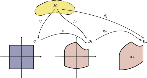
Figure 5.1: The pieces $M_{i}$ and the chart diagrams for $F_{\alpha},\,F_{i},\,g_{i}$ and $R_{\alpha}$.

By making $\rho$ small enough, one may assume that all $\Omega_{\beta}$, $\beta\in A^{\prime}$, intersecting an open set $\Omega_{\alpha}$ containing a node carry regular models. Thus we need to define transition functions between a regular model and a focus-focus model. On $\Delta_{\alpha\beta}:=\Omega_{\alpha}\cap\Omega_{\beta}$, both momentum maps $F_{\alpha}$ and $F_{\beta}$ are regular. Contrary to all previous cases, the focus-focus model $F_{\alpha}$ is not explicit, and we cannot simply provide an elementary formula for the transition map $\varphi_{\alpha\beta}$. However, since $C\setminus\ell$ is simply connected and a set of regular values of $F_{i}$, we can invoke the Liouville-Mineur-Arnold action-angle theorem and assert that there exists a symplectomorphism $\varphi_{i}:F_{i}^{-1}(C\setminus\ell)\rightarrow{\mathbb{T}}^{2}\times C^{\prime}\subset T^{*}{\mathbb{T}}^{2}=\{(x,\xi)\in\mathbb{T}^{2}\times\mathbb{R}^{2}\}$ such that

$$F_{i}=\varphi_{i}^{*}(h_{i}(\xi))\,\,\,\textup{for some diffeomorphism}\,\,\,h_{i}:C^{\prime}\rightarrow C\setminus\ell.$$

Then $\mu_{i}=\varphi_{i}^{*}(g_{i}\circ h_{i}(\xi))$. Since both $\mu_{i}$ and $\xi$ are toric momentum maps for the same foliation, there exists a transformation $H_{i}\in\textup{Aff}(2,\mathbb{Z})$ such that $g_{i}\circ h_{i}=H_{i}$.

Thus, if $F_{\alpha}$ is focus-focus and $F_{\beta}$ is regular, we introduce the symplectomorphism

$$\varphi_{\alpha\beta}:=\tilde{R}_{\beta}^{-1}\tilde{R}_{\alpha}\tilde{H}_{i}\circ\varphi_{i}\quad:F_{\alpha}^{-1}(\Delta_{\alpha\beta})\rightarrow F_{\beta}^{-1}(\Delta_{\alpha\beta}).$$ (5.8)

We verify $F_{\beta}\circ\varphi_{\alpha\beta}=F_{r}\circ\tilde{R}_{\beta}\circ\varphi_{\alpha\beta}=R_{\alpha}H_{i}F_{r}\circ\varphi_{i}=R_{\alpha}\mu_{i}=F_{\alpha}$, so we have shown (5.2).

We can now include these nodal pieces in the symplectic glueing construction using Theorem 3.10, which defines a symplectic manifold $M_{A^{\prime\prime}}$ and a proper map

$$F_{A^{\prime\prime}}\colon M_{A^{\prime\prime}}\to\bigcup_{\alpha\in A^{\prime\prime}}\Omega_{\alpha}\subset\mathbb{R}^{2}.$$

However $F_{A^{\prime\prime}}$ is not smooth everywhere, but it is a smooth toric momentum map outside the preimages of the cuts $\ell_{j}^{+}$ ($j=1,\dots,m_{f}$).

Third stage. Filling in the gaps.—

Here we add the open sets $\Omega_{\alpha}$ that were covering the cuts $\ell_{i}$ by switching these lines on the other side. Let $t_{i}:=t_{\ell_{\lambda_{i}}}$ as in Section 2.2. The cut $\ell_{i}^{+}$ is invariant under $t_{i}$. The open sets $t_{i}(\Omega_{\alpha})$, $\alpha\in A\setminus A^{\prime\prime}$ form a cover of $\ell_{i}\cap t_{i}(\Delta)$. Within the geometry of the new polygon $t_{i}(\Delta)$, each of these open sets can be associated with either a regular model, a transversally elliptic model, or an elliptic-elliptic model (indeed, under the transformation $t_{i}$, a fake corner disappears, and a hidden Delzant corner unhides itself.)

Thus we can add these to our glueing data, which amounts to equip each such open set $\Omega_{\alpha}$ with the model $(M_{\alpha},\,t_{i}^{-1}\circ F_{\alpha})$, where $(M_{\alpha},\,F_{\alpha})$ is determined as before, but for the transformed polygon $t_{i}(\Delta)$.

The transition maps are defined with the same formulas as before, taking into account that the map $R_{\alpha}$ is now a piecewise affine transformation. The cocycle conditions remain valid as well.

Doing this for all indices $i$, because all the $F_{\alpha}$ are continuous and proper, by Theorem 3.10, we obtain a smooth symplectic manifold $M=M_{A}$ equipped with a proper, continuous map $\mu=F_{A}$

$$\mu:M\rightarrow\bigcup_{\alpha\in A}\Omega_{\alpha}\subset\mathbb{R}^{2},$$ (5.9)

whose image is precisely $\Delta$.

However, the map $\mu$ is a proper toric momentum map only outside the cuts $\ell_{i}$. In other words, $\mu$ fails to be smooth along the cuts $\ell_{i}$. (Note that in the symplectic glueing construction, Theorem 3.10, we did not make any smoothness assumption on the $F_{\alpha}$, nor made any conclusion on the smoothness of $F$).

Fourth and final stage. Recovering smoothness.—

In this step we compose the final momentum map $\mu$ in (5.9) on the left by a suitable homeomorphism in order to make it smooth. Let $\Omega_{\alpha}$ be the open set containing the node $c_{i}$. Let $h_{i}=g_{i}^{-1}:D_{i}\rightarrow C$. The map $h_{i}$ is a bilipschitz homeomorphism fixing the origin and a smooth diffeomorphism outside the positive vertical axis. It is of the form

$$h_{i}(x,\,y)=(x,\,\eta_{i}(x,\,y)).$$

Since $h_{i}$ is orientation preserving, $\frac{\partial\eta_{i}}{\partial y}(x,\,y)>0$ for all $(x,\,y)\in D_{i}$. Let $\delta_{i}>0$ be such that $[-2\delta_{i},\,2\delta_{i}]^{2}\subset D_{i}$ and consider the vertical half-strip $\mathcal{S}_{\delta_{i}}:=[-\delta_{i},\,\delta_{i}]\times[-\delta_{i},\,\infty[$.

Claim 5.1.

There exists a function $\tilde{\eta}_{i}:D_{i}\rightarrow C$ such that

• $\tilde{\eta}_{i}(x,\,y)=\eta_{i}(x,\,y)$ for all $(x,\,y)\in D_{i}\cap\mathcal{S}_{\delta_{i}}$;

• $\tilde{\eta}_{i}(x,\,y)=y$ for all $(x,\,y)\in D_{i}\setminus\mathcal{S}_{2\delta_{i}}$;

• $\frac{\partial\tilde{\eta}_{i}}{\partial y}(x,\,y)>0$ for all $(x,\,y)\in D_{i}$.

In order to show this recall that if $f\colon A\to{\mathbb{R}}$ is smooth and $A\subset U\subset\mathbb{R}^{2}$ is closed, then $f$ has a smooth extension to $\tilde{f}\colon U\to\mathbb{R}$ where $U$ is open, see for example [22, Lem. 5.58 and Rmk. below it]. Let us apply this fact in our situation. Let $A_{\delta_{i}}:=(D_{i}\cap S_{\delta_{i}})\cup(D_{i}\setminus\!\!\mathop{\rm~{}Int}\nolimits(S_{\frac{3\delta_{i}}{2}})),$ which is a closed subset of $D_{i}\subset\mathbb{R}^{2}$, and let $\widehat{\eta}_{i}\colon A_{\delta_{i}}\to\mathbb{R}$ be the smooth function given by

$$\widehat{\eta}_{i}(x,\,y)=\left\{\begin{array}[]{rl}\eta_{i}(x,\,y)&\textup{ if }(x,\,y)\in\,D_{i}\cap\mathcal{S}_{\delta_{i}};\\ y&\textup{ if }(x,\,y)\in\,D_{i}\setminus\!\!\mathop{\rm~{}Int}\nolimits(\mathcal{S}_{\frac{3\delta_{i}}{2}}).\end{array}\right.$$ (5.12)

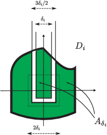
Figure 5.2: The set $A_{\delta_{i}}:=(D_{i}\cap S_{\delta_{i}})\cup(D_{i}\setminus\!\!\mathop{\rm~{}Int}\nolimits(S_{\frac{3\delta_{i}}{2}}))$, on which $\widehat{\eta}_{i}$ is defined.

Because $A_{\delta_{i}}\subset D_{i}$, and $D_{i}$ is bounded, there exists a constant $0<c_{i}<1$ such that $\frac{\partial\eta_{i}}{\partial y}>c$ on $A_{\delta_{i}}$ and hence $\frac{\partial\widehat{\eta}_{i}}{\partial y}>c_{i}\,\,\textup{on}\,\,A_{\delta_{i}}.$ Let $\zeta_{i}:=\frac{\partial\widehat{\eta}_{i}}{\partial y}-c_{i}\colon A_{\delta_{i}}\to\mathbb{R},$ which by assumption is strictly positive. By the above fact $\zeta_{i}$ extends to a smooth function $G_{i}:D_{i}\to\mathbb{R}$. Because the proof of the fact preserves non-negativity, and $\zeta_{i}>0$, we have that $G_{i}\geq 0$. By possibly shrinking the size of $D_{i}$ we can assume that $D_{i}$ is a disk of radius $r_{i}>0$ centered at the origin. Let $X_{\delta_{i}}:=[-r_{i},\,-\frac{3\delta_{i}}{2}]\cup[\frac{3\delta_{i}}{2},\,r_{i}]$, $Y_{\delta_{i}}:=[-\delta_{i},\,\delta_{i}]$, $Z_{\delta_{i}}:=[-\frac{3\delta_{i}}{2},\,-\delta_{i}]\cup[\delta_{i},\,\frac{3\delta_{i}}{2}]$ and let $\nu^{i}_{1}\colon X_{\delta_{i}}\to\mathbb{R}$ and $\nu^{i}_{2}\colon Y_{\delta_{i}}\to\mathbb{R}$ be the functions given by $\nu^{i}_{1}(x):=-\widehat{\eta}_{i}(x,\,0)$ and

$$\nu^{i}_{2}(x):=\widehat{\eta}_{i}(x,\,-\frac{3\delta_{i}}{2})-\int_{0}^{-\frac{3\delta_{i}}{2}}(G_{i}(x,\,t)+c_{i})\,\!\!\mathop{\rm~{}d}\nolimits\!t,$$

where we are using the convention $\int_{a}^{b}h=-\int_{b}^{a}h$ when $a>b$. Because $\widehat{\eta}_{i}$ and $G_{i}$ are smooth functions, $\nu^{i}_{1}$ and $\nu^{i}_{2}$ are also smooth. Let $\beta^{i}\colon[-r_{i},\,r_{i}]\to\mathbb{R}$ be a smooth extension of the function $X_{\delta_{i}}\cup Y_{\delta_{i}}\to\mathbb{R}$ defined by $\nu^{i}_{1}$ on $X_{\delta_{i}}$ and by $\nu^{i}_{2}$ on $Y_{\delta_{i}}$, which again exists by a partitions of unity argument.

Consider the function $\widetilde{\eta}_{i}\colon D_{i}\to\mathbb{R}$ given by

$$\widetilde{\eta}_{i}(x,\,y):=\beta^{i}(x)+\int_{0}^{y}(G_{i}(x,\,t)+c_{i})\,\!\!\mathop{\rm~{}d}\nolimits\!t.$$

Because $\beta$ is a smooth extension of $\nu^{i}_{1}$ and $\nu^{i}_{2}$, and $G$ is smooth, $\widetilde{\eta}_{i}$ is smooth. We claim that $\widetilde{\eta}_{i}|_{A_{\delta_{i}}}(x,\,y)=\widehat{\eta}_{i}(x,\,y)$ if $(x,\,y)\in A_{\delta_{i}}$. First assume $x\in Y_{\delta_{i}}$, and moreover that $-r_{i}\leq y\leq-\frac{3\delta_{i}}{2}$. Because $G_{i}$ is an extension of $g_{i}$ we have that

$$\widetilde{\eta}_{i}|_{A_{\delta_{i}}}(x,\,y)=\nu^{i}_{2}(x)+\Big{(}\int_{0}^{-\frac{3\delta_{i}}{2}}(G_{i}(x,\,t)+c_{i})\,\!\!\mathop{\rm~{}d}\nolimits\!t+\int_{-\frac{3\delta_{i}}{2}}^{y}\frac{\partial\widehat{\eta}_{i}}{\partial y}(x,\,t)\,\!\!\mathop{\rm~{}d}\nolimits\!t\Big{)},$$

and hence by the fundamental theorem of calculus, and using the definition of $\nu^{i}_{2}$ we obtain that

$$\widetilde{\eta}_{i}|_{A_{\delta_{i}}}(x,\,y)=\nu^{i}_{2}(x)+\Big{(}\int_{0}^{-\frac{3\delta_{i}}{2}}(G_{i}(x,\,t)+c_{i})\,\!\!\mathop{\rm~{}d}\nolimits\!t+(\widehat{\eta}_{i}(x,\,y)-\widehat{\eta}_{i}(x,\,-\frac{3\delta_{i}}{2}))\Big{)}=\widehat{\eta}_{i}(x,\,y).$$ (5.13)

The remaining subcases within the case of $x\in Y_{\delta_{i}}$ are when $-\delta_{i}\leq y\leq 0$, which follows by the same reasoning as in (a) using the formula for $\nu^{i}_{1}$ instead of $\nu^{i}_{2}$, the case of $0\leq y\leq r_{i}$, which is trivial because the extension is defined by the original function therein, and the case of $-\frac{3\delta_{i}}{2}\leq y\leq-\delta_{i}$, in which $(x,\,y)\notin A_{\delta_{i}}$ so there is nothing to prove. The case of $x\in X_{\delta_{i}}$ follows by the same type of argument as the case of $Y_{\delta_{i}}$. The case of $x\in Z_{\delta_{i}}$ is immediate because the extension is defined by the original function therein.

Applying again the fundamental theorem of calculus, because the functions $\nu^{i}_{1},\,\nu^{i}_{2},\,\beta^{i}$ do not depend on $y$, we have that

$$\frac{\partial\tilde{\eta}_{i}}{\partial y}=G_{i}+c_{i},$$ (5.14)

which is strictly positive since $G_{i}\geq 0$ and $c_{i}>0$. Because (5.14) and (5.13) hold we in turn have, in view of the definition (5.12) of $\widehat{\eta}$, that properties 1, 2, 3 are satisfied. This concludes the proof of Claim 5.1

Let $\Omega_{i}:=D_{i}\cup\{(x,\,y)\,|\,y<2\delta_{i}\}$. Because of the properties 1, 2, 3 of $\tilde{\eta}_{i}$, the map

$$\tilde{h}_{i}:(x,\,y)\mapsto(x,\tilde{\eta}_{i}(x,\,y))$$

coincides with $h_{i}$ in $\mathcal{S}_{\delta_{i}}$, while it is equal to the identity outside $\mathcal{S}_{2\delta_{i}}$. Thus we can extend it to $\Omega_{i}$ by letting it to be the identity outside $D_{i}\cup\mathcal{S}_{2\delta_{i}}$. We call this extension $\tilde{h}_{\Omega_{i}}$. Consider the map

$$\check{h}_{\Omega_{i}}:=\tilde{h}_{\Omega_{i}}\circ t_{0}^{-1},$$

where $t_{0}$ is the piecewise affine map $t_{\ell}$ with $\ell$ being the positive vertical axis. In $t_{0}(\Omega\cap\mathcal{S}_{\delta_{i}})$, it it equal to $h_{i}\circ t_{0}^{-1}$, which is now smooth outside the negative vertical axis (this follows from [20, Thm.  3.8]; also from the fact that it is the homeomorphism that one obtains in the construction of the generalized momentum map $t_{0}\circ g_{i}\circ F_{i}=t_{0}\circ\mu_{i}$: this amounts to switching the cut downwards.) Using the claim at the beginning of this step upside-down we can modify $\check{h}_{\Omega_{i}}$ in $\Omega_{i}\cap\{y>\delta_{i}\}$ in such a way that we can then extend it to be smooth on $t_{0}(\{y>\delta_{i}\})$. We obtain a homeomorphism of $\mathbb{R}^{2}$ that we call $(\check{h}_{\mathbb{R}^{2}})_{i}$.

Define the map $\varphi_{i}\colon\mathbb{R}^{2}\to\mathbb{R}^{2}$ by

$$\varphi_{i}:=R_{\alpha}\circ(\check{h}_{\mathbb{R}^{2}})_{i}\circ t_{0}\circ R_{\alpha}^{-1}.$$

Because $\varphi_{i}$ is a composite of homeomorphisms, it is a homeomorphism. Moreover, outside of $\mathcal{S}_{2\delta_{i}}$ we have that

$$\varphi_{i}=R_{\alpha}\circ(\check{h}_{\mathbb{R}^{2}})_{i}\circ t_{0}\circ R_{\alpha}^{-1}=R_{\alpha}\circ(\tilde{h}_{\Omega_{i}}\circ t_{0}^{-1})\circ t_{0}\circ R_{\alpha}^{-1},$$

and since $\tilde{h}_{\Omega_{i}}$ is the identity outside of $\mathcal{S}_{2\delta_{i}}$ we conclude that $\varphi_{i}$ is the identity map outside $\mathcal{S}_{2\delta_{i}}$. Now let $\varphi\colon\mathbb{R}^{2}\to\mathbb{R}^{2}$ be the piecewise defined map

$$\varphi(x,\,y):=\left\{\begin{array}[]{rl}\varphi_{i}(x,\,y)&\textup{ if }(x,\,y)\in\mathcal{S}_{2\delta_{i}};\\ (x,\,y)&\textup{ otherwise }.\end{array}\right.$$ (5.17)

Since each $\varphi_{i}$ is a homeomorphism, and equal to the identity outside of $\mathcal{S}_{2\delta_{i}}$, the formula (5.17) defines a homeomorphism.

Claim 5.2.

The map $\tilde{F}\colon M\to\mathbb{R}^{2}$ defined by $\tilde{F}:=\varphi\circ\mu$ is proper, and smooth everywhere.

The properness claim is immediate since $\varphi$ is a homeomorphism and $\mu$ is proper.

In order to show that $\tilde{F}$ is smooth, consider the map $\tilde{F}_{i}\colon M\to\mathbb{R}^{2}$ defined as a composite $\tilde{F}_{i}:=\varphi_{i}\circ\mu,$ where recall $\mu$ is the map (5.9). By definition of $\varphi$, we have that $\tilde{F}|_{\mathcal{S}_{\delta_{i}}}=\tilde{F}_{i}$, and hence to prove the claim it suffices to show that each $\tilde{F}_{i}$ is smooth. To prove this, we distinguish three cases.

Case 1: in a neighborhood of $c_{i}$. In the neighborhood $\Omega_{\alpha}$ of $c_{i}$ sent by $R_{\alpha}^{-1}$ into $[-\delta,\delta]^{2}$, we have that

$$(\check{h}_{\mathbb{R}^{2}})_{i}\,t_{0}\,R_{\alpha}^{-1}=\check{h}_{\Omega_{i}}\,t_{0}\,R_{\alpha}^{-1}=\tilde{h}_{\Omega_{i}}\,t_{0}^{-1}\,t_{0}\,R_{\alpha}^{-1}=h_{i}\,R_{\alpha}^{-1}.$$

Recall that $y_{\alpha}^{*}\mu=F_{\alpha}=R_{\alpha}\circ\mu_{i}$. Therefore one can write, in the preimage by $\mu$ of this neighbourhood, $y_{\alpha}^{*}(\tilde{F}_{i})=y_{\alpha}^{*}(h_{i}\circ\mu_{i})=F_{i}.$ Since $F_{i}$ is smooth, it follows that $\tilde{F}_{i}$ is smooth in $\Omega_{\alpha}$.

Case 2: away from the cut $\ell_{i}$. Let $\Lambda_{i}:=\bigcup_{j\neq i}\mu^{-1}(\ell_{j})\subset{\mathbb{R}}^{2}.$ We have that

$$(\check{h}_{\mathbb{R}^{2}})_{i}\,t_{0}\,R_{\alpha}^{-1}=\check{h}_{\Omega}\,t_{0}\,R_{\alpha}^{-1}=\tilde{h}_{\Omega}\,R_{\alpha}^{-1}\,\,\,\textup{on the set}\,\,\,(R_{\alpha}\circ t_{0}^{-1})(\{(x,\,y)\,|\,y<-\delta_{i}/2\}),$$

which by construction is smooth on this set. Thus $\tilde{F}_{i}$ has the same degree of smoothness as $\mu$ on the set $\mu^{-1}((R_{\alpha}\circ t_{0}^{-1})(\{(x,\,y)\,|\,y<-\delta/2\}))$. Note that the set $\mu^{-1}\big{(}(R_{\alpha}\circ t_{0}^{-1})(\{(x,\,y)\,|\,y<-\delta_{i}/2\})\big{)}$ does not contain $\mu^{-1}(\ell_{i})$. The same argument applies to the analogue subsets of $M$ corresponding to the regions $\{(x,\,y)\,|\,x<-\delta_{i}/2\}$ and $\{(x,\,y)\,|\,x>\delta_{i}/2\}$. On the subset of $M$ corresponding to the region $\{(x,\,y)\,|\,y>\delta_{i}/2\}$, the map $(\check{h}_{\mathbb{R}^{2}})_{i}$ is smooth by construction. Hence the map $\tilde{F}_{i}$ is smooth on $M\setminus\Lambda_{i}$.

Case 3: along the cut $\ell_{i}$, away from $c_{i}$. Remark that $t_{0}R_{\alpha}^{-1}=R_{\alpha}^{-1}t_{i}$. By construction of $\mu$ above the open sets $\Omega_{\beta}$ covering the cut $\ell_{i}$, we have that $y_{\beta}^{*}\,\mu=t_{i}^{-1}\,F_{\beta}.$ Hence

$$y_{\beta}^{*}((\check{h}_{\mathbb{R}^{2}})_{i}\,t_{0}\,R_{\alpha}^{-1}\mu)=y_{\beta}^{*}\,((\check{h}_{\mathbb{R}^{2}})_{i}\,F_{\beta})\,\,\,\textup{on the set}\,\,\,\mu^{-1}(\Omega_{\beta}),$$

and this expression defines a smooth map. Thus $\tilde{F}_{i}$ is smooth.

Hence putting cases 1, 2, 3 together we have shown that $\tilde{F}_{i}$ is smooth on $\mu^{-1}(\Omega_{\beta})$ for all $\Omega_{\beta}$ covering the cut $\ell_{i}$, and elsewhere, $\tilde{F}_{i}$ is as smooth as $\mu$. This concludes the proof of Claim 5.2.

Write $\tilde{F}:=(J,\,H)$. We then have the following conclusive claim.

Claim 5.3.

The symplectic manifold $(M,\ \omega)$ equipped with $J$ and $H$ is a semitoric integrable system. Moreover, the list of invariants (i)-(v) of the semitoric integrable system $(M,\,\omega,\,(J,\,H))$ is equal to the list of ingredients (i)-(v) that we started with. Finally, $M$ is a compact manifold if and only $\Delta$ is compact.

Let us prove this claim. We know from Claim 5.2 that $\tilde{F}$ is smooth. Since the first component $J$ is obtained from glueing proper maps, it follows from Theorem 3.10 that $J$ is proper. What’s more, the Hamiltonian flow of $J$ is everywhere periodic of period $2\pi$ because it is true in any local piece $M_{\alpha}$. Clearly $\{J,\,H\}=0$, since it is a local property. It is also easy to see that the only singularities of $\tilde{F}$ come from the singularities of the models $F_{\alpha}$, for the glueing procedure does not create any additional singularities. Now, near any elliptic critical value, the homeomorphism $\mu$ is a local diffeomorphism, so $\tilde{F}$ has the same singularity type as the elliptic model $F_{\alpha}$. Finally, near a node we have checked in the proof of Claim 5.2 that $\tilde{F}$ is precisely equal to the model $F_{i}$, and hence possesses a focus-focus singularity. Thus, provided we show that $M$ is connected, $(J,\,H)$ is a semitoric system.

Let us now consider its invariants (the connectedness of $M$ will follow).

• As we mentioned, the singularities of $\tilde{F}$ are only elliptic, except for the nodes $c_{1},\,\dots,\,c_{m_{f}}$ above each of which we have constructed a focus-focus singularity. Hence we have $m_{f}$ focus-focus singularities.

• Each focus-focus singularity was constructed by glueing a semi-local model with prescribed Taylor series invariant $(S_{i})^{\infty}$. Since this Taylor series is precisely a semi-local symplectic invariant, it is unchanged in the glued system $(M,\tilde{F})$.

• Thus we have a completely integrable system on $M$ that defines an integral affine structure (with boundary) on the image of $\tilde{F}$, except at the nodes $c_{i}$. For any choice of vertical half cuts $(\ell_{i},\epsilon_{i})$, the generalized momentum polygon is the image of the affine developing map. But the momentum map $\mu$, outside the focus-focus fibres, is precisely such a developing map and its image, by the glueing procedure, is the polygon $\Delta$. Hence the semitoric polygon invariant of $\tilde{F}$ is the orbit of $\Delta_{\!\!\mathop{\mbox{\rm\scriptsize~{}w}}\nolimits}$. (See Lemma 2.3.)

  Notice that this shows that the image of $\mu$ is connected, which implies that the total space $M$, obtained by glueing above the image of $\mu$, is connected as well.

• It follows directly from (iii) above and the definition of the nodes $c_{j}$ in (5.1) that the volume invariant defined in (2.10) is equal to $(h_{1},\dots,h_{m_{f}})$.

• We calculate the twisting indices of our semitoric system with respect to the fixed polygon $\Delta$ or, which amounts to the same, with respect to the toric momentum map $\mu$. By definition, the $j^{\!\!\mathop{\mbox{\rm\scriptsize~{}th}}\nolimits}$ twist is the integer $\tilde{k}_{j}$ such that

  $$\!\mathop{\rm d\!}\nolimits\mu=T^{\tilde{k}_{j}}\!\mathop{\rm d\!}\nolimits\mu_{j},$$

  where $\mu_{j}$ is the privileged momentum map of the focus-focus fibration above $c_{j}$. From the second stage of the construction, we know that

  $$\mu=F_{\alpha}=R_{\alpha}\circ\mu_{j}=\tau\circ T^{k_{j}}\circ\mu_{j},$$

  where $\tau$ is some translation. Hence $\!\mathop{\rm d\!}\nolimits\mu=T^{k_{j}}\!\mathop{\rm d\!}\nolimits\mu_{j}$, and thus $\tilde{k}_{j}=k_{j}$.

Thus we see that we could prove the second part of the claim because our construction is by symplectically glueing local pieces with the appropriate ingredients as in Definition 4.2. This is an advantage of constructing by glueing local pieces rather than, for example, a global reduction on a larger space.

This concludes the proof of Claim 5.3, and hence the proof of the theorem.

Alvaro Pelayo
University of California–Berkeley
Mathematics Department, 970 Evans Hall $\#$ 3840
Berkeley, CA 94720-3840, USA.
E-mail: apelayo@math.berkeley.edu

Vũ Ngọc San
Institut de Recherches Mathématiques de Rennes
Université de Rennes 1
Campus de Beaulieu
35042 Rennes cedex (France)
E-mail: san.vu-ngoc@univ-rennes1.fr

References

• [1] M. Atiyah: Convexity and commuting Hamiltonians. Bull. London Math. Soc. 14 (1982) 1–15.
• [2] N. Bourbaki: General Topology, Elements of Mathematics (Chapters I-IV) Springer, 1998
• [3] N. Bourbaki: Variétés différentielles et analytiques, Édition originale publiée par Masson, Paris, 1967.
• [4] H. Brandsma: Paracompactness, covers and perfect maps, Topology Explained, March 2003. Published by Topology Atlas. Available at: http://at.yorku.ca/p/a/c/a/00.htm
• [5] R.J. Daverman: Decompositions of Manifolds, AMS Bookstore 2007. Also published by Academic Press, Orlando, 1986.
• [6] T. Delzant: Hamiltoniens périodiques et image convexe de l’application moment. Bull. Soc. Math. France 116 (1988) 315–339.
• [7] J.J. Duistermaat. On global action-angle variables. Comm. Pure Appl. Math., 33:687–706, 1980.
• [8] J.P. Dufour and P. Molino. Compactification d’actions de $\mathbb{R}^{n}$ et variables actions-angles avec singularités. In Dazord and Weinstein, editors, Séminaire Sud-Rhodanien de Géométrie à Berkeley, volume 20, pages 151–167. MSRI, 1989.
• [9] L.H. Eliasson: Normal forms for Hamiltonian systems with Poisson commuting integrals – elliptic case, Comment. Math. Helv. 65 (1990), no. 1, 4 35; and Hamiltonian systems with Poisson commuting integrals, PhD thesis, University of Stockholm, 1984.
• [10] M. Gross and B. Siebert: Mirror symmetry via logarithmic degeneration data II, arXiv:0709.2290 [math.AG].
• [11] M. Gross and B. Siebert: From real affine geometry to complex geometry, arXiv:math/0703822 [math.AG].
• [12] M. Gross and B. Siebert: Mirror symmetry via logarithmic degeneration data I, J. Differential Geom. 72 (2006), 169 338. [math.AG/0309070].
• [13] M. Gross and B. Siebert: Affine manifolds, log structures, and mirror symmetry, Turkish J. Math. 27 (2003), 33 60. [math.AG/0211094].
• [14] V. Guillemin and S. Sternberg: Convexity properties of the moment mapping. Invent. Math. 67 (1982) 491–513.
• [15] N.C. Leung and M. Symington: Almost toric symplectic four-manifolds. arXiv:math.SG/0312165v1, 8 Dec 2003.
• [16] E. Miranda and N. T. Zung: Equivariant normal for for non-degenerate singular orbits of integrable Hamiltonian systems. Ann. Sci. École Norm. Sup. (4), 37(6):819–839, 2004.
• [17] A. Pelayo and S. Vũ Ngọc: Semitoric integrable systems on symplectic $4$-manifolds. Inventiones Math., to appear.
• [18] M. Symington: Four dimensions from two in symplectic topology. pp. 153–208 in Topology and geometry of manifolds (Athens, GA, 2001). Proc. Sympos. Pure Math., 71, Amer. Math. Soc., Providence, RI, 2003.
• [19] S. Vũ Ngọc: On semi-global invariants for focus-focus singularities. Top. 42 (2003), no. 2, 365–380.
• [20] S. Vũ Ngọc: Moment polytopes for symplectic manifolds with monodromy. Adv. Math. 208 (2007), no. 2, 909–934. 53D20
• [21] S. Willard: General Topology, Courier Dover Publications, 2004.
• [22] J.T. Wloka, B. Rowley and B. Lawruk: Boundary Value Problems for Elliptic Systems, Cambridge University Press 1995.
• [23] N.T. Zung: Symplectic topology of integrable hamiltonian systems, I: Arnold-Liouville with singularities, Compositio Math., vol. 101, p. 179–215, 1996.