Spectrum of large random reversible Markov chains: Heavy-tailed weights on the complete graph

Abstract

We consider the random reversible Markov kernel $K$ obtained by assigning i.i.d. nonnegative weights to the edges of the complete graph over $n$ vertices and normalizing by the corresponding row sum. The weights are assumed to be in the domain of attraction of an $\alpha$-stable law, $\alpha\in(0,2)$. When $1\leq\alpha<2$, we show that for a suitable regularly varying sequence $\kappa_{n}$ of index $1-1/\alpha$, the limiting spectral distribution $\mu_{\alpha}$ of $\kappa_{n}K$ coincides with the one of the random symmetric matrix of the un-normalized weights (Lévy matrix with i.i.d. entries). In contrast, when $0<\alpha<1$, we show that the empirical spectral distribution of $K$ converges without rescaling to a nontrivial law $\widetilde{\mu}_{\alpha}$ supported on $[-1,1]$, whose moments are the return probabilities of the random walk on the Poisson weighted infinite tree (PWIT) introduced by Aldous. The limiting spectral distributions are given by the expected value of the random spectral measure at the root of suitable self-adjoint operators defined on the PWIT. This characterization is used together with recursive relations on the tree to derive some properties of $\mu_{\alpha}$ and $\widetilde{\mu}_{\alpha}$. We also study the limiting behavior of the invariant probability measure of $K$.

, and

t1Supported in part by NSF Grant DMS-03-01795 and by the European Research Council through the “Advanced Grant” PTRELSS 228032.

1 Introduction

Let $G_{n}=(V_{n},E_{n})$ denote the complete graph with vertex set $V_{n}=\{1,\ldots,n\}$, and edge set $E_{n}=\{\{i,j\},1\leq i,j\leq n\}$, including loops $\{i,i\}$, $1\leq i\leq n$. Assign a nonnegative random weight (or conductance) $U_{i,j}=U_{j,i}$ to each edge $\{i,j\}\in E_{n}$, and assume that the symmetric weights $\mathbf{U}=\{U_{i,j};\{i,j\}\in E_{n}\}$ are i.i.d. with common law $\mathcal{L}$ independent of $n$. This defines a random network, or weighted graph, denoted $(G_{n},\mathbf{U})$. Next, consider the random walk on $(G_{n},\mathbf{U})$ defined by the transition probabilities

$$K_{i,j}:=\frac{U_{i,j}}{\rho_{i}}\qquad\mbox{with }\rho_{i}:=\sum_{j=1}^{n}U_{i,j}.$$ (1)

The Markov kernel $K$ is reversible with respect to the measure $\rho=\sum_{i\in V_{n}}\rho_{i}\delta_{i}$ in that

$$\rho_{i}K_{i,j}=\rho_{j}K_{j,i}$$

for all $i,j\in V_{n}$. Note that we have not assumed that $\mathcal{L}$ has no atom at $0$. If $\rho_{i}=0$ for some $i$, then for that index $i$ we set $K_{i,j}=\delta_{i,j}$, $1\leq j\leq n$. However, as soon as $\mathcal{L}$ is not concentrated at $0$ then almost surely, for all $n$ sufficiently large, $\rho_{i}>0$ for all $1\leq i\leq n$, $K$ is irreducible and aperiodic and $\rho$ is its unique invariant measure, up to normalization (see, e.g., bordenave-caputo-chafai ).

For any square $n\times n$ matrix $M$ with eigenvalues $\lambda_{1}(M),\ldots,\lambda_{n}(M)$, the Empirical Spectral Distribution (ESD) is the discrete probability measure with at most $n$ atoms defined by

$$\mu_{M}:=\frac{1}{n}\sum_{j=1}^{n}\delta_{\lambda_{j}(M)}.$$

All matrices $M$ to be considered in this work have real spectrum, and the eigenvalues will be labeled in such a way that $\lambda_{n}(M)\leq\cdots\leq\lambda_{1}(M)$.

Note that $K$ defines a square $n\times n$ random Markov matrix whose entries are not independent due the normalizing sums $\rho_{i}$. By reversibility, $K$ is self-adjoint in $L^{2}(\rho)$ and its spectrum $\sigma(K)$ is real. Moreover, $\sigma(K)\subset[-1,+1]$, and $1\in\sigma(K)$. Since $K$ is Markov, its ESD $\mu_{K}$ carries further probabilistic content. Namely, for any $\ell\in\mathbb{N}$, if $p_{\ell}(i)$ denotes the probability that the random walk on $(G_{n},\mathbf{U})$ started at $i$ returns to $i$ after $\ell$ steps, then the $\ell$th moment of $\mu_{K}$ satisfies

$$\int_{-1}^{+1}x^{\ell}\mu_{K}(dx)=\frac{1}{n}\operatorname{tr}(K^{\ell})=\frac{1}{n}\sum_{i\in V}p_{\ell}(i).$$ (2)

Convergence of the ESD

The asymptotic behavior of $\mu_{K}$ as $n\to\infty$ depends strongly on the tail of $\mathcal{L}$ at infinity. When $\mathcal{L}$ has finite mean $\int_{0}^{\infty}x\mathcal{L}(dx)=m$ we set $m=1$. This is no loss of generality since $K$ is invariant under the dilation $t\to tU_{i,j}$. If $\mathcal{L}$ has a finite second moment we write $\sigma^{2}=\int_{0}^{\infty}(x-1)^{2}\mathcal{L}(dx)$ for the variance.

The following result, from bordenave-caputo-chafai , states that if $0<\sigma^{2}<\infty$, then the bulk of the spectrum of $\sqrt{n}K$ behaves, when $n\to\infty$, as if we had truly i.i.d. entries (Wigner matrix). Without loss of generality, we assume that the weights $\mathbf{U}$ come from the truncation of a unique infinite table $(U_{i,j})_{{i,j}\geq 1}$ of i.i.d. random variables of law $\mathcal{L}$. This gives a meaning to the almost sure (a.s.) convergence of $\mu_{\sqrt{n}K}$. The symbol $\stackrel{{\scriptstyle w}}{{\to}}$ denotes weak convergence of measures with respect to continuous bounded functions. Note that $\lambda_{1}(\sqrt{n}K)=\sqrt{n}\to\infty$.

Theorem 1.1 ((Wigner-like behavior))

If $\mathcal{L}$ has variance $0<\sigma^{2}<\infty$, then a.s.

$$\mu_{\sqrt{n}K}:=\frac{1}{n}\sum_{k=1}^{n}\delta_{\sqrt{n}\lambda_{k}(K)}\mathop{\longrightarrow}^{w}_{n\to\infty}\mathcal{W}_{2\sigma},$$ (3)

where $\mathcal{W}_{2\sigma}$ is the Wigner semi-circle law on $[-2\sigma,+2\sigma]$. Moreover, if $\mathcal{L}$ has finite fourth moment, then $\lambda_{2}(\sqrt{n}K)$ and $\lambda_{n}(\sqrt{n}K)$ converge a.s. to the edge of the limiting support $[-2\sigma,+2\sigma]$.

This Wigner-like scenario can be dramatically altered if we allow $\mathcal{L}$ to have a heavy tail at infinity. For any $\alpha\in(0,\infty)$, we say that $\mathcal{L}$ belongs to the class $\mathbb{H}_{\alpha}$ if $\mathcal{L}$ is supported in $[0,\infty)$ and has a regularly varying tail of index $\alpha$, that is, for all $t>0$,

$$G(t):=\mathcal{L}((t,\infty))=L(t)t^{-\alpha},$$ (4)

where $L$ is a function with slow variation at $\infty$; that is, for any $x>0$,

$$\lim_{t\to\infty}\frac{L(xt)}{L(t)}=1.$$

Set $a_{n}=\inf\{a>0\dvtx nG(a)\leq 1\}$. Then $nG(a_{n})=nL(a_{n})a_{n}^{-\alpha}\to 1$ as $n\to\infty$, and

$$nG(a_{n}t)\to t^{-\alpha}\qquad\mbox{as }n\to\infty\mbox{ for all $t>0$}.$$ (5)

It is well known that $a_{n}$ has regular variation at $\infty$ with index $1/\alpha$, that is,

$$a_{n}=n^{1/\alpha}\ell(n)$$

for some function $\ell$ with slow variation at $\infty$ (see, e.g., Resnick resnick , Section 2.2.1). As an example, if $V$ is uniformly distributed on the interval $[0,1]$, then for every $\alpha\in(0,\infty)$, the law of $V^{-1/\alpha}$, supported in $[1,\infty)$, belongs to $\mathbb{H}_{\alpha}$. In this case, $L(t)=1$ for $t\geq 1$, and $a_{n}=n^{1/\alpha}$.

To understand the limiting behavior of the spectrum of $K$ in the heavy-tailed case it is important to consider first the symmetric i.i.d. matrix corresponding to the un-normalized weights $U_{i,j}$. More generally, we introduce the random $n\times n$ symmetric matrix $X$ defined by

$$X=(X_{i,j})_{1\leq{i,j}\leq n},$$ (6)

where $(X_{i,j})_{1\leq i\leq j\leq n}$ are i.i.d. such that $U_{i,j}:=|X_{i,j}|$ has law in $\mathbb{H}_{\alpha}$ with $\alpha\in(0,2)$, and

$$\theta=\lim_{t\to\infty}\frac{\mathbb{P}(X_{i,j}>t)}{\mathbb{P}(|X_{i,j}|>t)}\in[0,1].$$ (7)

It is well known that, for $\alpha\in(0,2)$, a random variable $Y$ is in the domain of attraction of an $\alpha$-stable law iff the law of $|Y|$ is in $\mathbb{H}_{\alpha}$ and the limit (7) exists (cf. Feller , Theorem IX.8.1a). It will be useful to view the entries $X_{i,j}$ in (6) as the marks across edge $\{i,j\}\in E_{n}$ of a random network $(G_{n},\mathbf{X})$, just as the marks $U_{i,j}$ defined the network $(G_{n},\mathbf{U})$ introduced above.

Remarkable works have been devoted recently to the asymptotic behavior of the ESD of matrices $X$ defined by (6), sometimes called Lévy matrices. The analysis of the Limiting Spectral Distribution (LSD) for $\alpha\in(0,2)$ is considerably harder than the finite second moment case (Wigner matrices), and the LSD is nonexplicit. Theorem 1.2 below has been investigated by the physicists Bouchaud and Cizeau BouchaudCizeau and rigorously proved by Ben Arous and Guionnet benarous-guionnet , and Belinschi, Dembo and Guionnet belinschi (see also Zakharevich zakharevich for related results).

Theorem 1.2 ([Symmetric i.i.d. matrix, $\alpha\in(0,2)$])

For every $\alpha\in(0,2)$, there exists a symmetric probability distribution $\mu_{\alpha}$ on $\mathbb{R}$ depending only on $\alpha$ such that [with the notation of (5) and (6)] a.s.

$$\mu_{a_{n}^{-1}X}:=\frac{1}{n}\sum_{i=1}^{n}\delta_{\lambda_{i}(a_{n}^{-1}X)}\mathop{\longrightarrow}^{w}_{n\to\infty}\mu_{\alpha}.$$

In Section 3.2, we give a new independent proof of Theorem 1.2. The key idea of our proof is to exhibit a limiting self-adjoint operator $\mathbf{T}$ for the sequence of matrices $a_{n}^{-1}X$, defined on a suitable Hilbert space, and then use known spectral convergence theorems of operators. The limiting operator will be defined as the “adjacency matrix” of an infinite rooted tree with random edge weights, the so-called Poisson weighted infinite tree (PWIT) introduced by Aldous aldous92 (see also aldoussteele ). In other words, the PWIT will be shown to be the local weak limit of the random network $(G_{n},\mathbf{X})$ when the edge marks $X_{i,j}$ are rescaled by $a_{n}$. In this setting the LSD $\mu_{\alpha}$ arises as the expected value of the (random) spectral measure of the operator $\mathbf{T}$ at the root of the tree. The PWIT and the limiting operator $\mathbf{T}$ are defined in Section 2. Our method of proof can be seen as a variant of the resolvent method, based on local convergence of operators. It is also well suited to investigate properties of the LSD $\mu_{\alpha}$ (cf. Theorem 1.6 below).

Let us now come back to our random reversible Markov kernel $K$ defined by (1) from weights with law $\mathcal{L}\in\mathbb{H}_{\alpha}$. We obtain different limiting behavior in the two regimes $\alpha\in(0,1)$ and $\alpha\in(1,2)$. The case $\alpha>2$ corresponds to a Wigner-type behavior (special case of Theorem 1.1). We set

$$\kappa_{n}=na_{n}^{-1}.$$

Theorem 1.3 ([Reversible Markov matrix, $\alpha\in(1,2)$])

Let $\mu_{\alpha}$ be the probability distribution which appears as the LSD in the symmetric i.i.d. case (Theorem 1.2). If $\mathcal{L}\in\mathbb{H}_{\alpha}$ with $\alpha\in(1,2)$ then a.s.

$$\mu_{\kappa_{n}K}:=\frac{1}{n}\sum_{k=1}^{n}\delta_{\lambda_{k}(\kappa_{n}K)}\mathop{\longrightarrow}^{w}_{n\to\infty}\mu_{\alpha}.$$

Theorem 1.4 ([Reversible Markov matrix, $\alpha\in(0,1)$])

For every $\alpha\in(0,1)$, there exists a symmetric probability distribution $\widetilde{\mu}_{\alpha}$ supported on $[-1,1]$ depending only on $\alpha$ such that a.s.

$$\mu_{K}:=\frac{1}{n}\sum_{k=1}^{n}\delta_{\lambda_{k}(K)}\mathop{\longrightarrow}^{w}_{n\to\infty}\widetilde{\mu}_{\alpha}.$$

The proofs of Theorems 1.3 and 1.4 are given in Sections 3.3 and 3.1, respectively. As in the proof of Theorem 1.2, the main idea is to exploit convergence of our matrices to suitable operators defined on the PWIT. To understand the scaling in Theorem 1.3, we recall that if $\alpha>1$, then by the strong law of large numbers, we have $n^{-1}\rho_{i}\to 1$ a.s. for every row sum $\rho_{i}$, and this is shown to remove, in the limit $n\to\infty$, all dependencies in the matrix $na_{n}^{-1}K$, so that we obtain the same behavior of the i.i.d. matrix of Theorem 1.2. On the other hand, when $\alpha\in(0,1)$, both the sum $\rho_{i}$ and the maximum of its elements are on scale $a_{n}$. The proof of Theorem 1.4 shows that the matrix $K$ converges (without rescaling) to a random stochastic self-adjoint operator $\mathbf{K}$ defined on the PWIT. The operator $\mathbf{K}$ can be described as the transition matrix of the simple random walk on the PWIT and is naturally linked to Poisson–Dirichlet random variables. This is based on the observation that the order statistics of any given row of the matrix $K$ converges weakly to the Poisson–Dirichlet law $\mathrm{PD}(\alpha,0)$ (see Lemma 2.4 below for the details). In fact, the operator $\mathbf{K}$ provides an interesting generalization of the Poisson–Dirichlet law.

Since $\mu_{K}$ is supported in $[-1,1]$, (2) and Theorem 1.4 imply that for all $\ell\geq 1$, a.s.

$$\frac{1}{n}\sum_{i=1}^{n}p_{\ell}(i)=\int_{\mathbb{R}}x^{\ell}\mu_{K}(dx)\mathop{\longrightarrow}_{n\to\infty}\int_{\mathbb{R}}x^{\ell}\widetilde{\mu}_{\alpha}(dx)=:\gamma_{\ell}.$$ (8)

The LSD $\widetilde{\mu}_{\alpha}$ will be obtained as the expectation of the (random) spectral measure of $\mathbf{K}$ at the root of the PWIT. It will follow that $\gamma_{\ell}$ (the $\ell$th moment of $\widetilde{\mu}_{\alpha}$) is the expected value of the (random) probability that the random walk returns to the root in $\ell$-steps. In particular, the symmetry of $\widetilde{\mu}_{\alpha}$ follows from the bipartite nature of the PWIT.

It was proved by Ben Arous and Guionnet benarous-guionnet , Remark 1.5, that $\alpha\in(0,2)\mapsto\mu_{\alpha}$ is continuous with respect to weak convergence of probability measures, and by Belinschi, Dembo and Guionnet belinschi , Remark 1.2 and Lemma 5.2, that $\mu_{\alpha}$ tends to the Wigner semi-circle law as $\alpha\nearrow 2$. We believe that Theorem 1.3 should remain valid for $\alpha=2$ with LSD given by the Wigner semi-circle law. Further properties of the measures $\mu_{\alpha}$ and $\widetilde{\mu}_{\alpha}$ are discussed below.

The case $\alpha=1$ is qualitatively similar to the case $\alpha\in(1,2)$ with the difference that the sequence $\kappa_{n}$ in Theorem 1.3 has to be replaced by $\kappa_{n}=na_{n}^{-1}w_{n}$ where

$$w_{n}=\int_{0}^{a_{n}}x\mathcal{L}(dx).$$ (9)

Indeed, here the mean of $U_{i,j}$ may be infinite and the closest one gets to a law of large numbers is the statement that $\rho_{i}/nw_{n}\to 1$ in probability (see Section 3.4). The sequence $w_{n}$ (and therefore $\kappa_{n}$) is known to be slowly varying at $\infty$ for $\alpha=1$ (see, e.g., Feller Feller , VIII.8). The following mild condition will be assumed: There exists $0<\varepsilon<1/2$ such that

$$\liminf_{n\to\infty}\frac{w_{\lfloor n^{\varepsilon}\rfloor}}{w_{n}}>0.$$ (10)

For example, if $U_{i,j}^{-1}$ is uniform on $[0,1]$, then $\kappa_{n}=w_{n}=\log n$ and$\lim_{n\to\infty}w_{\lfloor n^{\varepsilon}\rfloor}/w_{n}=\varepsilon$. In the next theorem $\mu_{1}$ stands for the LSD $\mu_{\alpha}$ from Theorem 1.2, at $\alpha=1$.

Theorem 1.5 ((Reversible Markov matrix, $\alpha=1$))

Suppose that $\mathcal{L}\in\mathbb{H}_{\alpha}$ with $\alpha=1$ and assume (10). If $\mu_{\kappa_{n}K}$ is the ESD of $\kappa_{n}K$, with $\kappa_{n}=na_{n}^{-1}w_{n}$, then, as $n\to\infty$, a.s. $\mu_{\kappa_{n}K}\mathop{\longrightarrow}\limits^{w}\limits_{n\to\infty}\mu_{1}$.

Properties of the LSD

In Section 4 we prove some properties of the LSDs $\mu_{\alpha}$ and $\widetilde{\mu}_{\alpha}$.

Theorem 1.6 ((Properties of $\mu_{\alpha}$))

Let $\mu_{\alpha}$ be the symmetric LSD in Theorems 1.2 and 1.3.

1. [(iii)]

2. $\mu_{\alpha}$ is absolutely continuous on $\mathbb{R}$.

3. The density of $\mu_{\alpha}$ at $0$ is equal to

   $$\frac{1}{\pi}\Gamma\biggl{(}1+\frac{2}{\alpha}\biggr{)}\biggl{(}\frac{\Gamma(1-{\alpha}/{2})}{\Gamma(1+{\alpha}/{2})}\biggr{)}^{{1}/{\alpha}}.$$

4. $\mu_{\alpha}$ is heavy tailed, and as $t$ goes to $+\infty$,

   $$\mu_{\alpha}((t,+\infty))\sim\tfrac{1}{2}t^{-\alpha}.$$

Statements (i) and (ii) answer some questions raised in benarous-guionnet , belinschi . Statement (iii) is already contained in belinschi , Theorem 1.7, but we provide a new proof based on a Tauberian theorem for the Cauchy–Stieltjes transform that may be of independent interest.

Theorem 1.7 ((Properties of $\widetilde{\mu}_{\alpha}$))

Let $\widetilde{\mu}_{\alpha}$ be the symmetric LSD in Theorem 1.4, with moments $\gamma_{\ell}$ as in (8). Then the following statements hold true.

1. [(iii)]

2. For $\alpha\in(0,1)$, there exists $\delta>0$ such that

   $$\gamma_{2n}\geq\delta n^{-\alpha}\qquad\mbox{for all }n\geq 1.$$

   Moreover, we have $\liminf_{\alpha\nearrow 1}\gamma_{2}>0$.

3. For the topology of the weak convergence, the map $\alpha\mapsto\widetilde{\mu}_{\alpha}$ is continuous in $(0,1)$.

4. For the topology of the weak convergence,

   $$\lim_{\alpha\searrow 0}\widetilde{\mu}_{\alpha}=\frac{1}{4}\delta_{-1}+\frac{1}{2}\delta_{0}+\frac{1}{4}\delta_{1}.$$

It is delicate to provide liable numerical simulations of the ESDs.

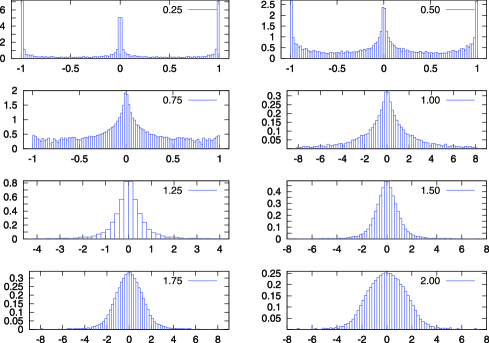
Figure 1: Histograms of scaled ESDs illustrating the convergence stated by Theorems 1.3 and 1.4, for the following values of $\alpha\dvtx 0.25$, $0.50$, $0.75$, $1.00$, $1.25$, $1.50$, $1.75$, $2.00$. Here $n=5000$ and $\mathcal{L}$ is the law of $V^{-1/\alpha}$ where $V$ is a uniform random variable on $(0,1)$. The first three plots are the histogram of the spectrum of a single realization of $K$. The fourth plot corresponds to $\alpha=1$ and is a histogram of the spectrum of a single realization of $\log(n)K$. The four last plots are the histogram of the spectrum of a single realization of $\kappa_{n}K$. In order to avoid scaling problems, an asymptotically negligible portion of the spectrum edge was discarded: only $\lambda_{\lfloor\log(n)\rfloor},\ldots,\lambda_{\lfloor n-\log(n)\rfloor}$ were used.

Nevertheless, Figure 1 provides histograms for various values of $\alpha$ and a large value of $n$, illustrating Theorems 1.3–1.7.

Invariant measure and edge behavior

Finally, we turn to the analysis of the invariant probability distribution $\hat{\rho}$ for the random walk on $(G,\mathbf{U})$. This is obtained by normalizing the vector of row sums $\rho$

$$\hat{\rho}=(\rho_{1}+\cdots+\rho_{n})^{-1}(\rho_{1},\ldots,\rho_{n}).$$

Following bordenave-caputo-chafai , Lemma 2.2, if $\alpha>2$, then $n\max_{1\leq i\leq n}|\hat{\rho}_{i}-n^{-1}|\to 0$ as $n\to\infty$ a.s. This uniform strong law of large numbers does not hold in the heavy-tailed case $\alpha\in(0,2)$: the large $n$ behavior of $\hat{\rho}$ is then dictated by the largest weights in the system.

Below we use the notation $\widetilde{\rho}=(\widetilde{\rho}_{1},\ldots,\widetilde{\rho}_{n})$ for the ranked values of $\hat{\rho}_{1},\ldots,\hat{\rho}_{n}$, so that $\widetilde{\rho}_{1}\geq\widetilde{\rho}_{2}\geq\cdots$ and their sum is $1$. The symbol $\stackrel{{\scriptstyle d}}{{\longrightarrow}}$ denotes convergence in distribution. We refer to Section 2.4 for more details on weak convergence in the space of ranked sequences and for the definition of the Poisson–Dirichlet law $\mathrm{PD}(\alpha,0)$.

Theorem 1.8 ((Invariant probability measure))

Suppose that $\mathcal{L}\in\mathbb{H}_{\alpha}$.

1. [(ii)]

2. If $\alpha\in(0,1)$, then

   $$\widetilde{\rho}\mathop{\longrightarrow}^{d}_{n\to\infty}\tfrac 12(V_{1},V_{1},V_{2},V_{2},\ldots),$$ (11)

   where $V_{1}>V_{2}>\cdots$ stands for a Poisson–Dirichlet $\mathrm{PD}(\alpha,0)$ random vector.

3. If $\alpha\in(1,2)$, then

   $$\kappa_{n(n+1)/2}\widetilde{\rho}\mathop{\longrightarrow}^{d}_{n\to\infty}\tfrac 12(x_{1},x_{1},x_{2},x_{2},\ldots),$$ (12)

   where $x_{1}>x_{2}>\cdots$ denote the ranked points of the Poisson point process on $(0,\infty)$ with intensity measure $\alpha x^{-\alpha-1}\,dx$. Moreover, the same convergence holds for $\alpha=1$ provided the sequence $\kappa_{n}$ is replaced by $na_{n}^{-1}w_{n}$, with $w_{n}$ as in (9).

Theorem 1.8 is proved in Section 5. These results will be derived from the statistics of the ranked values of the weights $U_{i,j}$, $i<j$, on the scale $a_{n(n+1)/2}$ (diagonal weights $U_{i,i}$ are easily seen to give negligible contributions). The duplication in the sequences in (12) and (11) then comes from the fact that each of the largest weights belongs to two distinct rows and determines alone the limiting value of the associated row sum.

Theorem 1.8 is another indication that the random walk with transition matrix $K$ shares the features of a trap model. Loosely speaking, instead of being trapped at a vertex, as in the usual mean field trap models (see Bouchaud , BenArousCerny , MR2152251 , MR2435851 ) here the walker is trapped at an edge.

Large edge weights are responsible for the large eigenvalues of $K$. This phenomenon is well understood in the case of symmetric random matrices with i.i.d. entries, where it is known that, for $\alpha\in(0,4)$, the edge of the spectrum gives rise to a Poisson statistics (see MR2081462 , auffinger-benarous-peche ). The behavior of the extremal eigenvalues of $K$ when $\mathcal{L}$ has finite fourth moment has been studied in bordenave-caputo-chafai . In particular, it is shown there that the spectral gap $1-\lambda_{2}$ is $1-O(n^{-1/2})$. In the present case of heavy-tailed weights, in contrast, by localization on the largest edge weight it is possible to prove that, a.s. and up to corrections with slow variation at $\infty$,

$$1-\lambda_{2}=\cases{O(n^{-1/\alpha}),&\quad$\alpha\in(0,1)$,\cr O\bigl{(}n^{-(2-\alpha)/\alpha}\bigr{)},&\quad$\alpha\in[1,2)$.}$$ (13)

Similarly, for $\alpha\in(2,4)$ one has that $\lambda_{2}$ is bounded below by $n^{-(\alpha-2)/\alpha}$. Understanding the statistics of the extremal eigenvalues remains an interesting open problem.

2 Convergence to the Poisson weighted infinite tree

The aim of this section is to prove that the matrices $X$ and $K$ appearing in Theorems 1.2, 1.3 and 1.4, when properly rescaled, converge “locally” to a limiting operator defined on the Poisson weighted infinite tree (PWIT). The concept of local convergence of operators is defined below. We first recall the standard construction of the PWIT.

2.1 The PWIT

Given a Radon measure $\nu$ on $\mathbb{R}$, $\operatorname{PWIT}(\nu)$ is the random rooted tree defined as follows. The vertex set of the tree is identified with $\mathbb{N}^{f}:=\bigcup_{k\in\mathbb{N}}\mathbb{N}^{k}$ by indexing the root as $\mathbb{N}^{0}=\varnothing$, the offsprings of the root as $\mathbb{N}$ and, more generally, the offsprings of some $\mathbf{v}\in\mathbb{N}^{k}$ as $(\mathbf{v}1),(\mathbf{v}2),\ldots\in\mathbb{N}^{k+1}$ [for short notation, we write $(\mathbf{v}1)$ in place of $(\mathbf{v},1)$]. In this way the set of $\mathbf{v}\in\mathbb{N}^{n}$ identifies the $n$th generation.

We now assign marks to the edges of the tree according to a collection $\{\Xi_{\mathbf{v}}\}_{\mathbf{v}\in\mathbb{N}^{f}}$ of independent realizations of the Poisson point process with intensity measure $\nu$ on $\mathbb{R}$. Namely, starting from the root $\varnothing$, let $\Xi_{\varnothing}=\{y_{1},y_{2},\ldots\}$ be ordered in such a way that $|y_{1}|\leq|y_{2}|\leq\cdots,$ and assign the mark $y_{i}$ to the offspring of the root labeled $i$. Now, recursively, at each vertex $\mathbf{v}$ of generation $k$, assign the mark $y_{\mathbf{v}i}$ to the offspring labeled $\mathbf{v}i$, where $\Xi_{\mathbf{v}}=\{y_{\mathbf{v}1},y_{\mathbf{v}2},\ldots\}$ satisfy $|y_{\mathbf{v}1}|\leq|y_{\mathbf{v}2}|\leq\cdots.$

2.2 Local operator convergence

We give a general formulation and later specialize to our setting. Let $V$ be a countable set, and let $L^{2}(V)$ denote the Hilbert space defined by the scalar product

$$\langle\phi,\psi\rangle:=\sum_{u\in V}\bar{\phi}_{u}\psi_{u},\qquad\phi_{u}=\langle\delta_{u},\phi\rangle,$$

where $\phi,\psi\in\mathbb{C}^{V}$ and $\delta_{u}$ denote the unit vector with support $u$. Let $\mathcal{D}$ denote the dense subset of $L^{2}(V)$ of vectors with finite support.

Definition 2.1 ((Local convergence)).

Suppose $\mathbf{S}_{n}$ is a sequence of bounded operators on $L^{2}(V)$, and $\mathbf{S}$ is a closed linear operator on $L^{2}(V)$ with dense domain $D(\mathbf{S})\supset\mathcal{D}$. Suppose further that $\mathcal{D}$ is a core for $\mathbf{S}$ (i.e., the closure of $\mathbf{S}$ restricted to $\mathcal{D}$ equals $\mathbf{S}$). For any $u,v\in V$ we say that $(\mathbf{S}_{n},u)$ converges locally to $(\mathbf{S},v)$ and write

$$(\mathbf{S}_{n},u)\to(\mathbf{S},v),$$

if there exists a sequence of bijections $\sigma_{n}\dvtx V\to V$ such that $\sigma_{n}(v)=u$ and, for all $\phi\in\mathcal{D}$,

$$\sigma_{n}^{-1}\mathbf{S}_{n}\sigma_{n}\phi\to\mathbf{S}\phi,$$

in $L^{2}(V)$, as $n\to\infty$.

In other words, this is the standard strong convergence of operators up to a re-indexing of $V$ which preserves a distinguished element. With a slight abuse of notation we have used the same symbol $\sigma_{n}$ for the linear isometry $\sigma_{n}\dvtx L^{2}(V)\to L^{2}(V)$ induced in the obvious way, that is, such that $\sigma_{n}\delta_{v}=\delta_{\sigma_{n}(v)}$ for all $v\in V$. The point for introducing Definition 2.1 lies in the following theorem on strong resolvent convergence. Recall that if $\mathbf{S}$ is a self-adjoint operator its spectrum is real, and for all $z\in\mathbb{C}_{+}:=\{z\in\mathbb{C}\dvtx\Im z>0\}$, the operator $\mathbf{S}-zI$ is invertible with bounded inverse. The operator-valued function $z\mapsto(\mathbf{S}-zI)^{-1}$ is the resolvent of $\mathbf{S}$.

Theorem 2.2 ((From local convergence to resolvents))

If $\mathbf{S}_{n}$ and $\mathbf{S}$ are self-adjoint operators that satisfy the conditions of Definition 2.1 and $(\mathbf{S}_{n},\break u)\to(\mathbf{S},v)$ for some $u,v\in V$, then, for all $z\in\mathbb{C}_{+}$,

$$\langle\delta_{u},(\mathbf{S}_{n}-zI)^{-1}\delta_{u}\rangle\to\langle\delta_{v},(\mathbf{S}-zI)^{-1}\delta_{v}\rangle.$$ (14)

It is a special case of reedsimon , Theorem VIII.25(a). Indeed, if we define $\widetilde{\mathbf{S}}_{n}=\sigma_{n}^{-1}\mathbf{S}_{n}\sigma_{n}$, then $\widetilde{\mathbf{S}}_{n}\phi\to\mathbf{S}\phi$ for all $\phi$ in a common core of the self-adjoint operators $\widetilde{\mathbf{S}}_{n},\mathbf{S}$. This implies the strong resolvent convergence, that is, $(\widetilde{\mathbf{S}}_{n}-zI)^{-1}\psi\to(\mathbf{S}-zI)^{-1}\psi$ for any $z\in\mathbb{C}_{+}$, $\psi\in L^{2}(V)$. The conclusion follows by taking the scalar product

$$\langle\delta_{v},(\widetilde{\mathbf{S}}_{n}-zI)^{-1}\delta_{v}\rangle=\langle\delta_{u},(\mathbf{S}_{n}-zI)^{-1}\delta_{u}\rangle.$$

We shall apply the above theorem in cases where the operators $\mathbf{S}_{n}$ and $\mathbf{S}$ are random operators on $L^{2}(V)$, which satisfy with probability one the conditions of Definition 2.1. In this case we say that $(\mathbf{S}_{n},u)\to(\mathbf{S},v)$ in distribution if there exists a random bijection $\sigma_{n}$ as in Definition 2.1 such that $\sigma_{n}^{-1}\mathbf{S}_{n}\sigma_{n}\phi$ converges in distribution to $\mathbf{S}\phi$, for all $\phi\in\mathcal{D}$ [where a random vector $\psi_{n}\in L^{2}(V)$ converges in distribution to $\psi$ if

$$\lim_{n\to\infty}\mathbb{E}f(\psi_{n})=\mathbb{E}f(\psi)$$

for all bounded continuous functions $f\dvtx L^{2}(V)\to\mathbb{R}$]. Under these assumptions then (14) becomes convergence in distribution of (bounded) complex random variables. In our setting the Hilbert space will be $L^{2}(V)$, with $V=\mathbb{N}^{f}$, the vertex set of the PWIT, the operator $\mathbf{S}_{n}$ will be a rescaled version of the matrix $X$ defined by (6) or the matrix $K$ defined by (1). The operator $\mathbf{S}$ will be the corresponding limiting operator defined below.

2.3 Limiting operators

Let $\theta$ be as in Theorem 1.2, and let $\ell_{\theta}$ be the positive Borel measure on the real line defined by $d\ell_{\theta}(x)=\theta\mathbh{1}_{\{x>0\}}\,dx+(1-\theta)\mathbh{1}_{\{x<0\}}\,dx$. Consider a realization of $\operatorname{PWIT}(\ell_{\theta})$. As before the mark from vertex $\mathbf{v}\in\mathbb{N}^{k}$ to $\mathbf{v}k\in\mathbb{N}^{k+1}$ is denoted by $y_{\mathbf{v}k}$. We note that almost surely

$$\sum_{k}|y_{\mathbf{v}k}|^{-2/\alpha}<\infty,$$ (15)

since a.s. $\lim_{k}|y_{\mathbf{v}k}|/k=1$ and $\sum_{k}k^{-2/\alpha}$ converges for $\alpha\in(0,2)$. Recall that for $V=\mathbb{N}^{f}$, $\mathcal{D}$ is the dense set of $L^{2}(V)$ of vectors with finite support. We may a.s. define a linear operator $\mathbf{T}\dvtx\mathcal{D}\to L^{2}(V)$ by letting, for $\mathbf{v},\mathbf{w}\in\mathbb{N}^{f}$,

$$\qquad\mathbf{T}(\mathbf{v},\mathbf{w}) = \langle\delta_{\mathbf{v}},\mathbf{T}\delta_{\mathbf{w}}\rangle$$

$$= \cases{\operatorname{sign}(y_{\mathbf{w}})|y_{\mathbf{w}}|^{-1/\alpha},&\quad if $\mathbf{w}=\mathbf{v}k$ for some integer $k$,\cr\operatorname{sign}(y_{\mathbf{v}})|y_{\mathbf{v}}|^{-1/\alpha},&\quad if $\mathbf{v}=\mathbf{w}k$ for some integer $k$,\cr 0,&\quad otherwise.}$$

Note that if every edge $e$ in the tree with mark $y_{e}$ is given the “weight” $\operatorname{sign}(y_{e})|y_{e}|^{-1/\alpha}$ then we may look at the operator $\mathbf{T}$ as the “adjacency matrix” of the weighted tree. Clearly, $\mathbf{T}$ is symmetric, and therefore it has a closed extension with domain $D(\mathbf{T})\subset L^{2}(\mathbb{N}^{f})$ such that $\mathcal{D}\subset D(\mathbf{T})$ (see, e.g., reedsimon , Chapter VIII, Section 2). We will prove in Proposition A.2 below that $\mathbf{T}$ is essentially self-adjoint, that is, the closure of $\mathbf{T}$ is self-adjoint. With a slight abuse of notation, we identify $\mathbf{T}$ with its closed extension. As stated below, $\mathbf{T}$ is the weak local limit of the sequence of $n\times n$ i.i.d. matrices $a_{n}^{-1}X$, where $X$ is defined by (6). To this end we view the matrix $X$ as an operator in $L^{2}(V)$ by setting $\langle\delta_{i},X\delta_{j}\rangle=X_{i,j}$, where $i,j\in\mathbb{N}$ denote the labels of the offsprings of the root (the first generation), with the convention that $X_{i,j}=0$ when either $i>n$ or $j>n$, and by setting $\langle\delta_{\mathbf{u}},X\delta_{\mathbf{v}}\rangle=0$ when either $\mathbf{u}$ or $\mathbf{v}$ does not belong to the first generation.

Similarly, taking now $\theta=1$, in the case of Markov matrices $K$ defined by (1), for $\alpha\in[1,2)$, $\mathbf{T}$ is the local limit operator of $\kappa_{n}K$. To work directly with symmetric operators we introduce the symmetric matrix

$$S_{i,j}=\frac{U_{i,j}}{\sqrt{\rho_{i}\rho_{j}}},$$ (17)

which is easily seen to have the same spectrum of $K$ (see, e.g., bordenave-caputo-chafai , Lemma 2.1). Again the matrix $S$ can be embedded in the infinite tree as described above for $X$.

In the case $\alpha\in(0,1)$ the Markov matrix $K$ has a different limiting object that is defined as follows. Consider a realization of $\operatorname{PWIT}(\ell_{1})$, where $\ell_{1}$ is the Lebesgue measure on $[0,\infty)$. We define an operator corresponding to the random walk on this tree with conductance equal to the mark to the power $-1/\alpha$. More precisely, for $\mathbf{v}\in\mathbb{N}^{f}$, let

$$\rho(\mathbf{v})=y^{-1/\alpha}_{\mathbf{v}}+\sum_{k\in\mathbb{N}}y^{-1/\alpha}_{\mathbf{v}k}$$

with the convention that $y^{-1/\alpha}_{\varnothing}=0$. Since a.s. $\lim_{k}|y_{\mathbf{v}k}|/k=1$, $\rho(\mathbf{v})$ is almost surely finite for $\alpha\in(0,1)$. We define the linear operator $\mathbf{K}$ on $\mathcal{D}$, by letting, for $\mathbf{v},\mathbf{w}\in\mathbb{N}^{f}$,

$$\qquad\mathbf{K}(\mathbf{v},\mathbf{w})=\langle\delta_{\mathbf{v}},\mathbf{K}\delta_{\mathbf{w}}\rangle=\cases{\dfrac{y^{-1/\alpha}_{\mathbf{w}}}{\rho(\mathbf{v})},&\quad if $\mathbf{w}=\mathbf{v}k$ for some integer $k$,\vspace*{2pt}\cr\dfrac{y^{-1/\alpha}_{\mathbf{v}}}{\rho(\mathbf{v})},&\quad if $\mathbf{v}=\mathbf{w}k$ for some integer $k$,\vspace*{2pt}\cr 0,&\quad otherwise.}$$ (18)

Note that $\mathbf{K}$ is not symmetric, but it becomes symmetric in the weighted Hilbert space $L^{2}(V,\rho)$ defined by the scalar product

$$\langle\phi,\psi\rangle_{\rho}:=\sum_{\mathbf{u}\in V}\rho(\mathbf{u})\bar{\phi}_{\mathbf{u}}\psi_{\mathbf{u}}.$$

Moreover, on $L^{2}(V,\rho)$, $\mathbf{K}$ is a bounded self-adjoint operator since Schwarz’s inequality implies

$$\langle\mathbf{K}\phi,\mathbf{K}\phi\rangle_{\rho}^{2} = \sum_{\mathbf{u}}\rho(\mathbf{u})\biggl{|}\sum_{\mathbf{v}}\mathbf{K}(\mathbf{u},\mathbf{v})\phi_{\mathbf{v}}\biggr{|}^{2}$$

$$\leq \sum_{\mathbf{u}}\rho(\mathbf{u})\sum_{\mathbf{v}}\mathbf{K}(\mathbf{u},\mathbf{v})|\phi_{\mathbf{v}}|^{2}$$

$$= \sum_{\mathbf{v}}\rho(\mathbf{v})|\phi_{\mathbf{v}}|^{2}=\langle\phi,\phi\rangle_{\rho}^{2}$$

so that the operator norm of $\mathbf{K}$ is less than or equal to $1$. To work with self-adjoint operators in the unweighted Hilbert space $L^{2}(V)$ we shall actually consider the operator $\mathbf{S}$ defined by

$$\mathbf{S}(\mathbf{v},\mathbf{w}):=\sqrt{\frac{\rho(\mathbf{v})}{\rho(\mathbf{w})}}\mathbf{K}(\mathbf{v},\mathbf{w})=\frac{\mathbf{T}(\mathbf{v},\mathbf{w})}{\sqrt{\rho(\mathbf{v})\rho(\mathbf{w})}}.$$ (19)

This defines a bounded self-adjoint operator in $L^{2}(V)$. Indeed, the map $\delta_{\mathbf{v}}\to\sqrt{\rho(\mathbf{v})}\delta_{\mathbf{v}}$ induces a linear isometry $\mathbf{D}\dvtx L^{2}(V,\rho)\to L^{2}(V)$ such that

$$\langle\phi,\mathbf{S}\psi\rangle=\langle\mathbf{D}^{-1}\phi,\mathbf{K}\mathbf{D}^{-1}\psi\rangle_{\rho},$$ (20)

for all $\phi,\psi\in L^{2}(V)$. In this way, when $\alpha\in(0,1)$, $\mathbf{S}$ will be the limiting operator associated with the matrix $S$ defined in (17). Note that no rescaling is needed here. The main result of this section is the following.

Theorem 2.3 ((Limiting operators))

As $n$ goes to infinity, in distribution:

1. [(iii)]

2. if $\alpha\in(0,2)$ and $\theta\in[0,1]$, then $(a_{n}^{-1}X,1)\to(\mathbf{T},\varnothing)$;

3. if $\alpha\in(1,2)$ and $\theta=1$, then $(\kappa_{n}S,1)\to(\mathbf{T},\varnothing)$;

4. if $\alpha\in(0,1)$, then $(S,1)\to(\mathbf{S},\varnothing)$.

From the remark after Theorem 2.2 we see that Theorem 2.3 implies convergence in distribution of the resolvent at the root. As we shall see in Section 3, this in turn gives convergence of the expected values of the Cauchy–Stieltjes transform of the ESD of our matrices. The rest of this section is devoted to the proof of Theorem 2.3.

2.4 Weak convergence of a single row

In this paragraph, we recall some facts about the order statistics of the first row of the matrix $X$ and $K$, that is,

$$(X_{1,1},\ldots,X_{1,n})\quad\mbox{and}\quad(U_{1,1},\ldots,U_{1,n})/\rho_{1},$$

where $U_{1,j}=|X_{1,j}|$ has law $\mathbb{H}_{\alpha}$. Let us denote by $V_{1}\geq V_{2}\geq\cdots\geq V_{n}$ the order statistics of the variables $U_{1,j}$, $1\leq j\leq n$. Recall that $\rho_{1}=\sum_{j=1}^{n}V_{j}$. Let us define $\Delta_{k,n}=\sum_{j=k+1}^{n}V_{j}$ for $k<n$ and $\Delta^{2}_{k,n}=\sum_{j=k+1}^{n}V_{j}^{2}$. Call $\mathcal{A}$ the set of sequences $\{v_{j}\}\in[0,\infty)^{\mathbb{N}}$ with $v_{1}\geq v_{2}\geq\cdots\geq 0$ such that $\lim_{j\to\infty}v_{j}=0$, and let $\mathcal{A}_{1}\subset\mathcal{A}$ be the subset of sequences satisfying $\sum_{j}v_{j}=1$. We shall view

$$Y_{n}=\biggl{(}\frac{V_{1}}{a_{n}},\ldots,\frac{V_{n}}{a_{n}}\biggr{)}\quad\mbox{and}\quad Z_{n}=\biggl{(}\frac{V_{1}}{\rho_{1}},\ldots,\frac{V_{n}}{\rho_{1}}\biggr{)}$$

as elements of $\mathcal{A}$ and $\mathcal{A}_{1}$, respectively, simply by adding zeros to the right of $V_{n}/a_{n}$ and $V_{n}/\rho_{1}$. Equipped with the standard product metric, $\mathcal{A}$ and $\mathcal{A}_{1}$ are complete separable metric spaces ($\mathcal{A}_{1}$ is compact), and convergence in distribution for $\mathcal{A},\mathcal{A}_{1}$-valued random variables is equivalent to finite-dimensional convergence (cf., e.g., Bertoin bertoin06 ).

Let $E_{1},E_{2},\ldots$ denote i.i.d. exponential variables with mean $1$ and write $\gamma_{k}=\sum_{j=1}^{k}E_{j}$. We define the random variable in $\mathcal{A}$

$$Y=(\gamma_{1}^{-1/\alpha},\gamma_{2}^{-1/\alpha},\ldots).$$

The law of $Y$ is the law of the ordered points of a Poisson process on $(0,\infty)$ with intensity measure $\alpha x^{-\alpha-1}\,dx$. For $\alpha\in(0,1)$ we define the variable in $\mathcal{A}_{1}$

$$Z=\biggl{(}\frac{\gamma_{1}^{-1/\alpha}}{\sum_{n=1}^{\infty}\gamma_{n}^{-1/\alpha}},\frac{\gamma_{2}^{-1/\alpha}}{\sum_{n=1}^{\infty}\gamma_{n}^{-1/\alpha}},\ldots\biggr{)}.$$

For $\alpha\in(0,1)$ the sum $\sum_{n}\gamma_{n}^{-1/\alpha}$ is a.s. finite. The law of $Z$ in $\mathcal{A}_{1}$ is called the Poisson–Dirichlet law $\mathrm{PD}(\alpha,0)$ (see Pitman and Yor MR1434129 , Proposition 10). The next result is rather standard but we give a simple proof for convenience.

Lemma 2.4 ((Poisson–Dirichlet laws and Poisson point processes))

1. [(iii)]

2. For all $\alpha>0$, $Y_{n}$ converges in distribution to $Y$. Moreover, for $\alpha\in(0,2)$, $(a_{n}^{-1}V_{j})_{j\geq 1}$ is a.s. uniformly square integrable, that is, a.s.$\lim_{k}\sup_{n>k}a_{n}^{-2}\times\Delta^{2}_{k,n}=0$.

3. If $\alpha\in(0,1)$, $Z_{n}$ converges in distribution to $Z$. Moreover, $(a_{n}^{-1}V_{j})_{j\geq 1}$ is a.s. uniformly integrable, that is, a.s. $\lim_{k}\sup_{n>k}a_{n}^{-1}\Delta_{k,n}=0$.

4. If $I\subset\mathbb{N}$ is a finite set and $V^{I}_{1}\geq V^{I}_{2}\geq\cdots$ denote the order statistics of $\{U_{1,j}\}_{j\in\{1,\ldots,n\}\setminus I}$ then (i) and (ii) hold with $Y^{I}_{n}=(V^{I}_{1}/a_{n},V^{I}_{2}/a_{n},\ldots)$ and $Z^{I}_{n}=(V^{I}_{1}/\rho_{1},V^{I}_{2}/\rho_{1},\ldots)$.

As an example, from (i), we retrieve the well-known fact that for any $\alpha>0$, the random variable $a_{n}^{-1}\max(U_{1,1},\ldots,U_{1,n})$ converges weakly as $n\to\infty$ to the law of $\gamma_{1}^{-1/\alpha}$. This law, known as a Fréchet law, has density $\alpha x^{-\alpha-1}e^{-x^{-\alpha}}$ on $(0,\infty)$. Proof of Lemma 2.4 As in LePage, Woodroofe and Zinn zinn81 we take advantage of the following well-known representation for the order statistics of i.i.d. random variables. Let $G$ be the function in (4) and write

$$G^{-1}(u)=\inf\{y>0\dvtx G(y)\leq u\},$$

$u\in(0,1)$. We have that $(V_{1},\ldots,V_{n})$ equals in distribution the vector

$$\bigl{(}G^{-1}(\gamma_{1}/\gamma_{n+1}),\ldots,G^{-1}(\gamma_{n}/\gamma_{n+1})\bigr{)},$$ (21)

where $\gamma_{j}$ has been defined above. To prove (i) we start from the distributional identity

$$Y_{n}\stackrel{{\scriptstyle d}}{{=}}\biggl{(}\frac{G^{-1}(\gamma_{1}/\gamma_{n+1})}{a_{n}},\ldots,\frac{G^{-1}(\gamma_{n}/\gamma_{n+1})}{a_{n}}\biggr{)},$$

which follows from (21). It suffices to prove that for every $k$, almost surely the first $k$ terms above converge to the first $k$ terms in $Y$. Thanks to (5), almost surely, for every $j$,

$$a_{n}^{-1}G^{-1}(\gamma_{j}/\gamma_{n+1})\to\gamma_{j}^{-1/\alpha},$$ (22)

and the convergence in distribution of $Y_{n}$ to $Y$ follows. Moreover, from (5), for any $\delta>0$ we can find $n_{0}$ such that

$$a_{n}^{-1}V_{j}=a_{n}^{-1}G^{-1}(\gamma_{j}/\gamma_{n+1})\leq\bigl{(}n\gamma_{j}/(1+\delta)\gamma_{n+1}\bigr{)}^{-1/\alpha},$$

for $n\geq n_{0}$, $j\in\mathbb{N}$. Since $n/\gamma_{n+1}\to 1$, a.s. we see that the expression above is a.s. bounded by $2(1+\delta)^{1/\alpha}\gamma_{j}^{-1/\alpha}$, for $n$ sufficiently large, and the second part of (i) follows from a.s. summability of $\gamma_{j}^{-2/\alpha}$.

Similarly, if $\alpha\in(0,1)$, $\Delta_{k,n}$ has the same law of

$$\sum_{j=k+1}^{n}G^{-1}(\gamma_{j}/\gamma_{n+1}),$$

and the second part of (ii) follows from a.s. summability of $\gamma_{j}^{-1/\alpha}$. To prove the convergence of $Z_{n}$ we use the distributional identity

$$Z_{n}\stackrel{{\scriptstyle d}}{{=}}\biggl{(}\frac{G^{-1}(\gamma_{1}/\gamma_{n+1})}{\sum_{j=1}^{n}G^{-1}(\gamma_{j}/\gamma_{n+1})},\ldots,\frac{G^{-1}(\gamma_{n}/\gamma_{n+1})}{\sum_{j=1}^{n}G^{-1}(\gamma_{j}/\gamma_{n+1})}\biggr{)}.$$

As a consequence of (22), we then have almost surely

$$a_{n}^{-1}\sum_{j=1}^{n}G^{-1}(\gamma_{j}/\gamma_{n+1})\to\sum_{j=1}^{\infty}\gamma_{j}^{-1/\alpha},$$

and (ii) follows. Finally, (iii) is an easy consequence of the exchangeability of the variable $(U_{1,i})$

$$\mathbb{P}(V^{I}_{k}\neq V_{k})\leq\mathbb{P}(\exists j\in I\dvtx U_{1,j}\geq V_{k})\leq|I|\mathbb{P}(U_{1,1}\geq V_{k})=|I|\frac{k}{n}.$$

The intensity measure $\alpha x^{-\alpha-1}\,dx$ on $(0,\infty)$ is not locally finite at $0$. It will be more convenient to work with Radon (i.e., locally finite) intensity measures.

Lemma 2.5 ((Poisson point processes with Radon intensity measures))

Let $\xi^{n}_{1},\xi^{n}_{2},\ldots$ be sequences of i.i.d. random variables on $\overline{\mathbb{R}}:=\mathbb{R}\cup\{\pm\infty\}$ such that

$$n\mathbb{P}(\xi^{n}_{1}\in\cdot)\mathop{\longrightarrow}^{w}_{n\to\infty}\nu,$$ (23)

where $\nu$ is a Radon measure on $\mathbb{R}$. Then, for any finite set $I\subset\mathbb{N}$ the random measure

$$\sum_{i\in\{1,\ldots,n\}\setminus I}\delta_{\xi^{n}_{i}}$$

converges weakly as $n\to\infty$ to $\operatorname{PPP}(\nu)$, the Poisson point process on $\mathbb{R}$ with intensity law $\nu$, for the usual vague topology on Radon measures.

We refer to resnick , Theorem 5.3, page 138, for a proof of Lemma 2.5. Note that for $\xi^{(n)}_{j}=a_{n}/U_{1,j}$ it is a consequence of Lemma 2.4(iii). In the case $\xi^{(n)}_{j}=a_{n}/X_{1,j}$, where $X_{i,j}$ is as in (6) and (7), the above lemma yields convergence to PPP($\nu_{\alpha,\theta}$), where

$$\nu_{\alpha,\theta}(dx)=\bigl{[}\theta\mathbh{1}_{\{x>0\}}+(1-\theta)\mathbh{1}_{\{x<0\}}\bigr{]}\alpha|x|^{\alpha-1}\,dx.$$ (24)

2.5 Local weak convergence to PWIT

In the previous paragraph we have considered the convergence of the first row of the matrix $a_{n}^{-1}X$. Here we generalize this by characterizing the limiting local structure of the complete graph with marks $a_{n}/X_{i,j}$. Our argument is based on a technical generalization of an argument borrowed from Aldous aldous92 . This will lead us to Theorems 2.3 and 2.8 below.

Let $G_{n}$ be the complete network on $\{1,\ldots,n\}$ whose mark on edge $(i,j)$ equals $\xi^{n}_{i,j}$, for some collection $(\xi^{n}_{ij})_{1\leq i\leq j\leq n}$ of i.i.d. random variables with values in $\mathbb{R}$, with $\xi^{n}_{j,i}=\xi^{n}_{i,j}$. We consider the rooted network $(G_{n},1)$ obtained by distinguishing the vertex labeled $1$.

We follow Aldous aldous92 , Section 3. For every fixed realization of the marks $(\xi^{n}_{ij})$, and for any $B,H\in\mathbb{N}$, such that $(B^{H+1}-1)/(B-1)\leq n$, we define a finite rooted subnetwork $(G_{n},1)^{B,H}$ of $(G_{n},1)$, whose vertex set coincides with a $B$-ary tree of depth $H$ with root at $1$.

To this end we partially index the vertices of $(G_{n},1)$ as elements in

$$J_{B,H}=\bigcup_{\ell=0}^{H}\{1,\ldots,B\}^{\ell}\subset\mathbb{N}^{f},$$

the indexing being given by an injective map $\sigma_{n}$ from $J_{B,H}$ to $V_{n}:=\{1,\ldots,n\}$. The map $\sigma_{n}$ can be extended to a bijection from a subset of $\mathbb{N}^{f}$ to $V_{n}$. We set $I_{\varnothing}=\{1\}$ and the index of the root $1$ is $\sigma_{n}^{-1}(1)=\varnothing$. The vertex $v\in V_{n}\setminus I_{\varnothing}$ is given the index $(k)=\sigma_{n}^{-1}(v)$, $1\leq k\leq B$, if $\xi^{n}_{(1,v)}$ has the $k$th smallest absolute value among $\{\xi^{n}_{1,j},j\neq 1\}$, the marks of edges emanating from the root $1$. We break ties by using the lexicographic order. This defines the first generation. Now let $I_{1}$ be the union of $I_{\varnothing}$ and the $B$ vertices that have been selected. If $H\geq 2$, we repeat the indexing procedure for the vertex indexed by $(1)$ (the first child) on the set $V_{n}\setminus I_{1}$. We obtain a new set $\{11,\ldots,1B\}$ of vertices sorted by their weights as before [for short notation, we concatenate the vector $(1,1)$ into $11$]. Then we define $I_{2}$ as the union of $I_{1}$ and this new collection. We repeat the procedure for $(2)$ on $V_{n}\setminus I_{2}$ and obtain a new set $\{21,\ldots,2B\}$, and so on. When we have constructed $\{B1,\ldots,BB\}$, we have finished the second generation (depth $2$) and we have indexed $(B^{3}-1)/(B-1)$ vertices. The indexing procedure is then repeated until depth $H$ so that $(B^{H+1}-1)/(B-1)$ vertices are sorted. Call this set of vertices $V_{n}^{B,H}=\sigma_{n}J_{B,H}$. The subnetwork of $G_{n}$ generated by $V_{n}^{B,H}$ is denoted $(G_{n},1)^{B,H}$ (it can be identified with the original network $G_{n}$ where any edge $e$ touching the complement of $V_{n}^{B,H}$ is given a mark $x_{e}=\infty$). In $(G_{n},1)^{B,H}$, the set $\{\mathbf{u}1,\ldots,\mathbf{u}B\}$ is called the set of children or offsprings of the vertex $\mathbf{u}$. Note that while the vertex set has been given a tree structure, $(G_{n},1)^{B,H}$ is still a complete network. The next proposition shows that it nevertheless converges to a tree (i.e., all circuits vanish, or equivalently, the extra marks diverge to $\infty$) if the $\xi^{n}_{i,j}$ satisfy a suitable scaling assumption.

Let $(\mathcal{T},\varnothing)$ denote the infinite random rooted network with distribution $\operatorname{PWIT}(\nu)$. We call $(\mathcal{T},\varnothing)^{B,H}$ the finite random network obtained by the sorting procedure described in the previous paragraph. Namely, $(\mathcal{T},\varnothing)^{B,H}$ consists of the sub-tree with vertices of the form $\mathbf{u}\in J_{B,H}$, with the marks inherited from the infinite tree. If an edge is not present in $(\mathcal{T},\varnothing)^{B,H}$, we assign to it the mark $+\infty$.

We say that the sequence of random finite networks $(G_{n},1)^{B,H}$ converges in distribution (as $n\to\infty$) to the random finite network $(\mathcal{T},\varnothing)^{B,H}$ if the joint distributions of the marks converge weakly. To make this precise we have to add the points $\{\pm\infty\}$ as possible values for each mark, and continuous functions on the space of marks have to be understood as functions such that the limit as any one of the marks diverges to $+\infty$ exists and coincides with the limit as the same mark diverges to $-\infty$. The next proposition generalizes aldous92 , Section 3.

Proposition 2.6 ((Local weak convergence to a tree))

Let $(\xi^{n}_{i,j})_{1\leq i\leq j\leq n}$ be a collection of i.i.d. random variables with values in $\overline{\mathbb{R}}:=\mathbb{R}\cup\{\pm\infty\}$ and set $\xi^{n}_{j,i}=\xi^{n}_{i,j}$. Let $\nu$ be a Radon measure on $\mathbb{R}$ with no mass at $0$ and assume that

$$n\mathbb{P}(\xi^{n}_{12}\in\cdot)\mathop{\longrightarrow}^{w}_{n\to\infty}\nu\qquad\mbox{as }n\to\infty.$$ (25)

Let $G_{n}$ be the complete network on $\{1,\ldots,n\}$ whose mark on edge $(i,j)$ equals $\xi^{n}_{ij}$. Then, for all integers $B,H$, as $n$ goes to infinity, in distribution,

$$(G_{n},1)^{B,H}\longrightarrow(\mathcal{T},\varnothing)^{B,H}.$$

Moreover, if $\mathcal{T}_{1},\mathcal{T}_{2}$ are independent with common law $\operatorname{PWIT}(\nu)$, then, in distribution,

$$((G_{n},1)^{B,H},(G_{n},2)^{B,H})\longrightarrow((\mathcal{T}_{1},\varnothing)^{B,H},(\mathcal{T}_{2},\varnothing)^{B,H}).$$

The second statement is the convergence of the joint law of the finite networks, where $(G_{n},2)^{B,H}$ is obtained with the same procedure as for $(G_{n},1)^{B,H}$, by starting from the vertex $2$ instead of $1$. In particular, the second statement implies the first.

This type of convergence is often referred to as local weak convergence, a notion introduced by Benjamini and Schramm benjaminischramm and Aldous and Steele aldoussteele (see also Aldous and Lyons aldouslyons ). Let us give some examples of application of this proposition. Consider the case where $\xi^{n}_{ij}=1$ with probability $\lambda/n$ and $\xi^{n}_{i,j}=\infty$ otherwise. The network $G_{n}$ is an Erdős–Rényi random graph with parameter $\lambda/n$. From the proposition, we retrieve the well-known fact that it locally converges to the tree of a Yule process of intensity $\lambda$. If $\xi^{n}_{i,j}=nY_{i,j}$, where $Y_{i,j}$ is any nonnegative continuous random variable with density $1$ at $0+$, then the network converges to $\operatorname{PWIT}(\ell_{1})$, where $\ell_{1}$ is the Lebesgue measure on $[0,\infty)$. The relevant application for our purpose is given by the choice $\xi^{n}_{i,j}=(a_{n}/X_{i,j})$, and $\nu=\nu_{\alpha,\theta}$, where $X_{i,j}$ are such that $|X_{i,j}|\in\mathbb{H}_{\alpha}$ and (7) is satisfied, and $\nu_{\alpha,\theta}$ is defined by (24). Note that the proposition applies to all $\alpha>0$ in this setting. Proof of Proposition 2.6 We order the elements of $J_{B,H}$ in the lexicographic order, that is, $\varnothing\prec 1\prec 2\prec\cdots\prec B\prec 11\prec 12\prec\cdots\prec B\cdots B$. For $\mathbf{v}\in J_{B,H}$, let $O_{\mathbf{v}}$ denote the set of offsprings of $\mathbf{v}$ in $(G_{n},1)^{B,H}$. By construction, we have $I_{\varnothing}=\{1\}$ and $I_{\mathbf{v}}=\sigma_{n}(\bigcup_{\mathbf{w}\prec\mathbf{v}}O_{\mathbf{w}})$. At every step of the indexing procedure, we sort the marks of the neighboring edges that have not been explored at an earlier step $\{1,\ldots,n\}\setminus I_{1}$, $\{1,\ldots,n\}\setminus I_{2},\ldots.$ Therefore, for all $\mathbf{u}$,

$$\bigl{(}\xi^{n}_{\sigma_{n}(\mathbf{u}),i}\bigr{)}_{i\notin I_{\mathbf{u}}}\stackrel{{\scriptstyle d}}{{=}}(\xi^{n}_{1,i})_{1\leq i\leq n-|I_{\mathbf{u}}|}.$$ (26)

Thus, from Lemma 2.5 and the independence of the variables $\xi^{n}$, we infer that the marks from a parent to its offsprings in $(G_{n},1)^{B,H}$ converge weakly to those in $(\mathcal{T},\varnothing)^{B,H}$. We now check that all other marks diverge to infinity. For $\mathbf{v},\mathbf{w}\in J_{B,H}$, we define

$$x^{n}_{\mathbf{v},\mathbf{w}}=\xi^{n}_{\sigma_{n}(\mathbf{v}),\sigma_{n}(\mathbf{w})}.$$

Also, let $\{y^{n}_{\mathbf{v},\mathbf{w}},\mathbf{v},\mathbf{w}\in J_{B,H}\}$ denote independent variables distributed as $|\xi^{n}_{1,2}|$. Let $E^{B,H}$ denote the set of edges $\{\mathbf{u},\mathbf{v}\}\in J_{B,H}\times J_{B,H}$ that do not belong to the finite tree (i.e., there is no $k\in\{1,\ldots,B\}$ such that $\mathbf{u}=\mathbf{v}k$ or $\mathbf{v}=\mathbf{u}k$). Lemma 2.7 below implies that the vector $\{|x^{n}_{\mathbf{v},\mathbf{w}}|,\{\mathbf{v},\mathbf{w}\}\in E^{B,H}\}$ stochastically dominates the vector $\mathcal{Y}^{n}:=\{y^{n}_{\mathbf{v},\mathbf{w}},\{\mathbf{v},\mathbf{w}\}\in E^{B,H}\}$, that is, there exists a coupling of the two vectors such that almost surely $|x^{n}_{\mathbf{v},\mathbf{w}}|\geq y^{n}_{\mathbf{v},\mathbf{w}}$, for all $\{\mathbf{v},\mathbf{w}\}\in E^{B,H}$. Since $J_{B,H}$ is finite (independent of $n$), $\mathcal{Y}^{n}$ contains a finite number of variables and (25) implies that the probability of the event $\{\min_{\{\mathbf{v},\mathbf{w}\}\in E^{B,H}}|x^{n}_{\mathbf{v},\mathbf{w}}|\leq t\}$ goes to $0$ as $n\to\infty$, for any $t>0$. Therefore it is now standard to obtain that if $x_{e}$ denote the mark of edge $e$ in $\mathcal{T}^{B,H}$, the finite collection of marks $(x^{n}_{e})_{e\in J_{B,H}\times J_{B,H}}$ converges in distribution to $(x_{e})_{e\in J_{B,H}\times J_{B,H}}$ as $n\to\infty$. In other words, $(G_{n},1)^{B,H}$ converges in distribution to $(\mathcal{T},\varnothing)^{B,H}$.

It remains to prove the second statement. It is an extension of the above argument. We consider the two subnetworks $(G_{n},1)^{B,H}$ and $(G_{n},2)^{B,H}$ obtained from $(G_{n},1)$ and $(G_{n},2)$. This gives rise to two increasing sequences of sets of vertices $I_{\mathbf{v},1}$ and $I_{\mathbf{v},2}$ with $\mathbf{v}\in J_{B,H}$ and two injective maps $\sigma_{n,1}$, $\sigma_{n,2}$ from $J_{B,H}$ to $\{1,\ldots,n\}$. We need to show that, in distribution,

$$((G_{n},1)^{B,H},(G_{n},2)^{B,H})\longrightarrow((\mathcal{T}_{1},\varnothing)^{B,H},(\mathcal{T}_{2},\varnothing)^{B,H}).$$ (27)

Let $V_{n,i}^{B,H}=\sigma_{n,i}(J_{B,H})$ be the vertex set of $(G_{n},i)^{B,H}$, $i=1,2$. There are

$$C:=\frac{B^{H+1}-1}{B-1}$$

vertices in $V_{n,i}^{B,H}$, hence the exchangeability of the variables implies that

$$\mathbb{P}(2\in V_{n,1}^{B,H})\leq\frac{C}{n}.$$

Let $\widetilde{G}_{n}=G_{n}\setminus V_{n,1}^{B,H}$, the subnetwork of $G_{n}$ spanned by the vertex set $V\setminus V^{B,H}_{n,1}$. Assuming that $2(B^{H+1}-1)/(B-1)<n$ and $2\notin V_{n,1}^{B,H}$, we may then define $(\widetilde{G}_{n},2)^{B,H}$. If $2\in V_{n,1}^{B,H}$, $(\widetilde{G}_{n},2)^{B,H}$ is defined arbitrarily. The above analysis shows that, in distribution,

$$((G_{n},1)^{B,H},(\widetilde{G}_{n},2)^{B,H})\longrightarrow((\mathcal{T}_{1},\varnothing)^{B,H},(\mathcal{T}_{2},\varnothing)^{B,H}).$$

Therefore in order to prove (27) it is sufficient to prove that with probability tending to $1$,

$$V_{n,1}^{B,H}\cap V_{n,2}^{B,H}=\varnothing.$$

Indeed, on the event $\{V_{n,1}^{B,H}\cap V_{n,2}^{B,H}=\varnothing\}$, $(G_{n},2)^{B,H}$ and $(\widetilde{G}_{n},2)^{B,H}$ are equal. For $\mathbf{v}\in J_{B,H}$, let $O_{\mathbf{v},2}$ denote the set of offsprings of $\mathbf{v}$ in $(G_{n},2)^{B,H}$. We have

$$I_{\mathbf{v},2}=\{2\}\cup\bigcup_{\mathbf{w}\prec\mathbf{v}}O_{\mathbf{w},2}$$

and

$$\mathbb{P}(V_{n,1}^{B,H}\cap V_{n,2}^{B,H}\neq\varnothing)$$

$$\qquad\leq\mathbb{P}(2\in V_{n,1}^{B,H})+\sum_{\mathbf{v}=\varnothing}^{B\cdots B}\mathbb{P}(O_{\mathbf{v},2}\cap V_{n,1}^{B,H}\neq\varnothing|V_{n,1}^{B,H}\cap I_{\mathbf{v},2}=\varnothing).$$

For any $\mathbf{u},\mathbf{v}\in J_{B,H}$, if $V_{n,1}^{B,H}\cap I_{\mathbf{v},2}=\varnothing$, then $\sigma_{n,2}(\mathbf{v})$ is neither the ancestor of $\sigma_{n,1}(\mathbf{u})$, nor an offspring of $\sigma_{n,1}(\mathbf{u})$. From Lemma 2.7 below we deduce that $|\xi^{n}_{\sigma_{n,1}(\mathbf{u}),\sigma_{n,2}(\mathbf{v})}|$ given $V_{n,1}^{B,H}\cap I_{\mathbf{v},2}=\varnothing$ dominates stochastically $|\xi^{n}_{1,2}|$, and is independent of the i.i.d. vector $(|\xi^{n}_{\sigma_{n,2}(\mathbf{v}),k}|)_{k\in\{1,\ldots,n\}\setminus(V_{n,1}^{B,H}\cup I_{\mathbf{v},2})}$, with law $|\xi^{n}_{1,2}|$. It follows that

$$\mathbb{P}\bigl{(}\sigma_{n,1}(\mathbf{u})\in O_{\mathbf{v},2}|V_{n,1}^{B,H}\cap I_{\mathbf{v},2}=\varnothing\bigr{)}\leq\frac{B}{n-C-|I_{\mathbf{v},2}|}.$$

Therefore,

$$\mathbb{P}(O_{\mathbf{v},2}\cap V_{n,1}^{B,H}\neq\varnothing|V_{n,1}^{B,H}\cap I_{\mathbf{v},2}=\varnothing)$$

$$\qquad\leq\sum_{\mathbf{u}\in J_{B,H}}\mathbb{P}\bigl{(}\sigma_{n,1}(\mathbf{u})\in O_{\mathbf{v},2}|V_{n,1}^{B,H}\cap I_{\mathbf{v},2}=\varnothing\bigr{)}$$

$$\qquad\leq\frac{CB}{n-2C}.$$

Finally,

$$\mathbb{P}(V_{n,1}^{B,H}\cap V_{n,2}^{B,H}\neq\varnothing)\leq\frac{C}{n}+\frac{C^{2}B}{n-2C},$$

which converges to $0$ as $n\to\infty$.

We have used the following stochastic domination lemma. For any $B,H$ and $n$ let $\mathcal{E}_{n}^{H,B}$ denote the (random) set of edges $\{i,j\}$ of the complete graph on $\{1,\ldots,n\}$, such that $\{\sigma_{n}^{-1}(i),\sigma_{n}^{-1}(j)\}$ is not an edge of the finite tree on $J_{B,H}$. By construction, any loop $\{i,i\}$ belongs to $\mathcal{E}_{n}^{B,H}$. Also, for $\mathbf{u}\neq\varnothing$ on the finite tree, let $g(\mathbf{u})$ denote the parent of $\mathbf{u}$.

Lemma 2.7 ((Stochastic domination))

For any $n\in\mathbb{N}$, and $B,H\in\mathbb{N}$ such that

$$\frac{B^{H+1}-1}{B-1}\leq n,$$

the random variables

$$\{|\xi^{n}_{i,j}|,\{i,j\}\in\mathcal{E}_{n}^{B,H}\}$$

stochastically dominate i.i.d. random variables with the same law as law $|\xi^{n}_{1,2}|$. Moreover, for every $\varnothing\neq\mathbf{u}\in J_{B,H}$, the random variables

$$\bigl{\{}\bigl{|}\xi^{n}_{\sigma_{n}(\mathbf{u}),i}\bigr{|},i\in\{1,\ldots,n\}\setminus\sigma_{n}(g(\mathbf{u}))\bigr{\}},$$

stochastically dominate i.i.d. random variables with the same law as law $|\xi^{n}_{1,2}|$.

The censoring process which deletes the edges that belong to the tree on $J_{B,H}$ has the property that at each step the $B$ lowest absolute values are deleted from some fresh (previously unexplored) subset of edge marks. Using this and the fact that the edge marks $\xi^{n}_{i,j}$ are i.i.d. we see that both claims in the lemma are implied by the following simple statement.

Let $Y_{1},\ldots,Y_{m}$ denote i.i.d. positive random variables. Suppose $m=n_{1}+\cdots+n_{\ell}$, for some positive integers $\ell$, $n_{1},\ldots,n_{\ell}$, and partition the $m$ variables in $\ell$ blocks $I^{1},\ldots,I^{\ell}$ of $n_{1},\ldots,n_{\ell}$ variables each. Fix some nonnegative integers $k_{j}$ such that $k_{j}\leq n_{j}$ and call $q_{1}^{j},\ldots,q^{j}_{k_{j}}$, the (random) indexes of the $k_{j}$ lowest values of the variables in the block $I^{j}$ (so that $Y_{q^{1}_{1}}$ is the lowest of the $Y_{1},\ldots,Y_{n_{1}}$, $Y_{q^{1}_{2}}$ is the second lowest of the $Y_{1},\ldots,Y_{n_{1}}$ and so on). Consider the random index sets of the $k_{j}$ minimal values in the $j$th block, $J^{j}:=\bigcup_{i=1}^{k_{j}}\{q^{j}_{i}\}$, and set $J=\bigcup_{j=1}^{\ell}J^{j}$. If $k_{j}=0$ we set $J^{j}=\varnothing$. Finally, let $\widetilde{Y}$ denote the vector $\{Y_{i},i=1,\ldots,m;i\notin J\}$. Then we claim that $\widetilde{Y}$ stochastically dominates $m-\sum_{j=1}^{\ell}k_{j}$ i.i.d. copies of $Y_{1}$.

Indeed, the coupling can be constructed as follows. We first extract a realization $y_{1},\ldots,y_{m}$ of the whole vector. Given this we isolate the index sets $J^{1},\ldots,J^{\ell}$ within each block. We then consider two vectors $\mathcal{Z},\mathcal{V}$ obtained as follows. The vector $\mathcal{Z}_{1}=(z^{1}_{1},\ldots,z^{1}_{n_{1}-k_{1}},z^{2}_{1},\ldots,z^{2}_{n_{2}-k_{2}},\ldots,z^{\ell}_{n_{\ell}-k_{\ell}})$ is obtained by extracting the $n_{1}-k_{1}$ values $z^{1}_{1},\ldots,z^{1}_{n_{1}-k_{1}}$ uniformly at random (without replacement) from the values $y_{1},\ldots,y_{n_{1}}$ (in the block $I^{1}$), the $n_{2}-k_{2}$ variables $z^{2}_{1},\ldots,z^{2}_{n_{2}-k_{2}}$ in the same way from the values $y_{n_{1}+1},\ldots,y_{n_{1}+n_{2}}$ (in the block $I^{2}$), and so on. On the other hand, the vector $\mathcal{V}=(v^{1}_{1},\ldots,v^{1}_{n_{1}-k_{1}},v^{2}_{1},\ldots,v^{2}_{n_{2}-k_{2}},\ldots,v^{\ell}_{n_{\ell}-k_{\ell}})$ is obtained as follows. For the first block we take $v^{1}_{i}$, $i=1,\ldots,n_{1}-k_{1}$ equal to $z^{1}_{i}$ whenever an index $i\in I^{1}\setminus J^{1}$ was picked for the vector $z^{1}_{1},\ldots,z^{1}_{n_{1}-k_{1}}$, and we assign the remaining values (if any) through an independent uniform permutation of those variables $y_{i},i\in I^{1}\setminus J^{1}$ which were not picked for the vector $z^{1}_{1},\ldots,z^{1}_{n_{1}-k_{1}}$. We repeat this procedure for all other blocks to assign all values of $\mathcal{V}$. By construction, $\mathcal{V}\geq\mathcal{Z}$ coordinate-wise. The conclusion follows from the observation that $\mathcal{Z}$ is distributed like a vector of $m-\sum_{j=1}^{\ell}k_{j}$ i.i.d. copies of $Y_{1}$, while $\mathcal{V}$ is distributed like our vector $\widetilde{Y}$.

2.6 Proof of Theorem 2.3

Proof of Theorem 2.3(i) Let $\nu=\nu_{\alpha,\theta}$ be as in (24), and let $(\mathcal{T}_{\alpha},\varnothing)$ be a realization of the $\operatorname{PWIT}(\nu)$. The mark on edge $(\mathbf{v},\mathbf{v}k)$ in $\mathcal{T}_{\alpha}$ is denoted by $x_{(\mathbf{v},\mathbf{v}k)}$ or simply $x_{\mathbf{v}k}$. By definition, we have $x_{(\mathbf{v},\mathbf{w})}=\infty$ if $\mathbf{v}$ and $\mathbf{w}$ are at graph-distance different from $1$. In particular, if we set $y_{\mathbf{v}}=\operatorname{sign}(x_{\mathbf{v}})|x_{\mathbf{v}}|^{\alpha}$, then the point sets $\Xi_{\mathbf{v}}=\{y_{\mathbf{v}k}\}_{k\geq 1}$ are independent Poisson point processes of intensity $\ell_{\theta}=\theta\mathbh{1}_{\{x>0\}}\,dx+(1-\theta)\mathbh{1}_{\{x<0\}}\,dx$. We may thus build a realization of the operator $\mathbf{T}$ on $\mathcal{T}_{\alpha}$ [cf. (2.3)]. Let $G_{n}$ be the complete network on $\{1,\ldots,n\}$ whose mark on edge $(i,j)$ is $\xi^{n}_{i,j}:=a_{n}/X_{i,j}$. Next, we apply Proposition 2.6. For all $B$, $H$, $(G_{n},1)^{B,H}$ converges weakly to $(\mathcal{T}_{\alpha},\varnothing)^{B,H}$. Let $\sigma_{n}^{B,H}$ be the map $\sigma_{n}$ associated with the network $(G_{n},1)^{B,H}$ (see the construction given before Proposition 2.6). From the Skorokhod representation theorem we may assume that $(G_{n},1)^{B,H}$ converges a.s. to $(\mathcal{T}_{\alpha},\varnothing)^{B,H}$ for all $B,H$. Thus we may find sequences $B_{n},H_{n}$ tending to infinity, such that $(B_{n}^{H_{n}+1}-1)/(B_{n}-1)\leq n$ and such that for any pair $\mathbf{u},\mathbf{v}\in\mathbb{N}^{f}$ we have $\xi^{n}_{(\widetilde{\sigma}_{n}(\mathbf{u}),\widetilde{\sigma}_{n}(\mathbf{v}))}\to x_{(\mathbf{u},\mathbf{v})}$ a.s. as $n\to\infty$, where $\widetilde{\sigma}_{n}:=\sigma_{n}^{B_{n},H_{n}}$. The map $\widetilde{\sigma}_{n}$ can be extended to a bijection $\mathbb{N}^{f}\to\mathbb{N}^{f}$. It follows that a.s.

$$\langle\delta_{\mathbf{u}},\widetilde{\sigma}_{n}^{-1}(a_{n}^{-1}X)\widetilde{\sigma}_{n}\delta_{\mathbf{v}}\rangle=\frac{1}{\xi^{n}_{(\widetilde{\sigma}_{n}(\mathbf{u}),\widetilde{\sigma}_{n}(\mathbf{v}))}}\to\frac{1}{x_{(\mathbf{u},\mathbf{v})}}=\langle\delta_{\mathbf{u}},\mathbf{T}\delta_{\mathbf{v}}\rangle.$$ (28)

Fix $\mathbf{v}\in\mathbb{N}^{f}$, and set $\psi_{n}^{\mathbf{v}}:=\widetilde{\sigma}_{n}^{-1}(a_{n}^{-1}X)\widetilde{\sigma}_{n}\delta_{\mathbf{v}}$. To prove Theorem 2.3(i) it is sufficient to show that $\psi_{n}^{\mathbf{v}}\to\mathbf{T}\delta_{\mathbf{v}}$ in $L^{2}(\mathbb{N}^{f})$ almost surely as $n\to\infty$, that is,

$$\sum_{\mathbf{u}}(\langle\delta_{\mathbf{u}},\psi_{n}^{\mathbf{v}}\rangle-\langle\delta_{\mathbf{u}},\mathbf{T}\delta_{\mathbf{v}}\rangle)^{2}\to 0.$$ (29)

Since from (28) we know that $\langle\delta_{\mathbf{u}},\psi_{n}^{\mathbf{v}}\rangle\to\langle\delta_{\mathbf{u}},\mathbf{T}\delta_{\mathbf{v}}\rangle$ for every $\mathbf{u}$, the claim follows if we have (almost surely) uniform (in $n$) square-integrability of $(\langle\delta_{\mathbf{u}},\psi_{n}^{\mathbf{v}}\rangle)_{\mathbf{u}}$. This in turn follows from Lemmas 2.7 and 2.4(i). The proof of Theorem 2.3(i) is complete. Proof of Theorem 2.3(ii) We need the following two facts:

$$\lim_{n\to\infty}\frac{\rho_{1}}{n}=1\qquad\mbox{in probability},$$ (30)

and there exists $\delta>0$ such that

$$\liminf_{n\to\infty}\min_{1\leq i\leq n}\frac{\rho_{i}}{n}>\delta\qquad\mbox{a.s.}$$ (31)

Clearly, (30) is a law of large numbers and holds actually a.s. (recall that for $\alpha>1$ we assume the mean of $U_{i,j}$ to be $1$). Let us establish the a.s. uniform bound (31). For every $\epsilon>0$, there exists $R>0$ such that $\mathbb{E}(U_{i,j}\mathbh{1}_{\{U_{i,j}<R\}})\geq 1-\epsilon$. If we define $\rho_{i}^{R}=\sum_{j=1}^{n}U_{i,j}\mathbh{1}_{\{U_{i,j}<R\}}$, then

$$\liminf_{n\to\infty}\min_{1\leq i\leq n}\frac{\rho_{i}}{n}\geq\liminf_{n\to\infty}\min_{1\leq i\leq n}\frac{\rho_{i}^{R}}{n}.$$

Therefore (31) is implied by the uniform law of large numbers in bordenave-caputo-chafai , Lemma 2.2, applied to the bounded variables $U_{i,j}\mathbh{1}_{\{U_{i,j}<R\}}$.

Next, we claim that for all $\mathbf{u}\in\mathbb{N}^{f}$, in probability

$$\lim_{n\to\infty}\frac{\rho_{\widetilde{\sigma}_{n}(\mathbf{u})}}{n}=1.$$ (32)

To prove this we first observe that by Lemma 2.7 and (30) we have in probability

$$\limsup_{n\to\infty}\frac{(\rho_{\widetilde{\sigma}_{n}(\mathbf{u})}-U_{\widetilde{\sigma}_{n}(\mathbf{u}),\widetilde{\sigma}_{n}(g(\mathbf{u}))})}{n}\leq 1.$$

On the other hand $U_{\widetilde{\sigma}_{n}(\mathbf{u}),\widetilde{\sigma}_{n}(g(\mathbf{u}))}$ is stochastically dominated by the maximum of $n$ i.i.d. variables with law $U_{i,j}$. The latter converges in distribution on the scale $a_{n}$ [cf. Lemma 2.4(i)], and we know that $a_{n}/n\to 0$. It follows that in probability $\limsup_{n\to\infty}\rho_{\widetilde{\sigma}_{n}(\mathbf{u})}/n\leq 1$. Next, we can estimate

$$\rho_{\widetilde{\sigma}_{n}(\mathbf{u})}\geq\sum_{i\in\{1,\ldots,n\}\setminus I_{\mathbf{u}}}U_{\widetilde{\sigma}_{n}(\mathbf{u}),i}.$$

Now, observe that if $\mathbf{u}\in\mathbb{N}^{f}$ belongs to generation $h$, then the set $I_{\mathbf{u}}$ contains at most $O(B_{n}^{h})$ elements, while $n$ is at least of order $B_{n}^{H_{n}}$, where $B_{n},H_{n}$ are the sequences used in the proof of Theorem 2.3(i). In particular, it follows that $|I_{\mathbf{u}}|=o(n)$ and therefore (26) and (30) imply that $\liminf_{n\to\infty}\rho_{\widetilde{\sigma}_{n}(\mathbf{u})}/n\geq 1$ in probability. This proves (32).

Thanks to (32), from the Slutsky lemma and the Skorokhod representation theorem, we may also assume that for each $\mathbf{v}\in\mathbb{N}^{f}$, $\rho_{\widetilde{\sigma}_{n}(\mathbf{v})}/n$ converges a.s. to $1$. We need to show that for each $\mathbf{v}\in\mathbb{N}^{f}$, (29) holds with the new vector $\psi_{n}^{\mathbf{v}}:=\widetilde{\sigma}_{n}^{-1}(\kappa_{n}S)\widetilde{\sigma}_{n}\delta_{\mathbf{v}}$,

$$\langle\delta_{\mathbf{w}},\psi_{n}^{\mathbf{v}}\rangle=\kappa_{n}\frac{U_{\widetilde{\sigma}_{n}(\mathbf{w}),\widetilde{\sigma}_{n}(\mathbf{v})}}{\sqrt{\rho_{\widetilde{\sigma}_{n}(\mathbf{v})}\rho_{\widetilde{\sigma}_{n}(\mathbf{w})}}}.$$

Thanks to (31), $(\langle\delta_{\mathbf{w}},\psi_{n}^{\mathbf{v}}\rangle)_{\mathbf{w}}$ is uniformly square-integrable [cf. the proof of (29)], and all we have to check is that $(\langle\delta_{\mathbf{w}},\psi_{n}^{\mathbf{v}}\rangle-\langle\delta_{\mathbf{w}},\mathbf{T}\delta_{\mathbf{v}}\rangle)^{2}\to 0$ for fixed $\mathbf{w}$. Here $\mathbf{T}$ is the operator appearing in the proof of Theorem 2.3(i) above, now with the choice $\theta=1$. We have

$$(\langle\delta_{\mathbf{w}},\psi_{n}^{\mathbf{v}}\rangle-\langle\delta_{\mathbf{w}},\mathbf{T}\delta_{\mathbf{v}}\rangle)^{2}$$

$$\qquad\leq 2\bigl{(}a_{n}^{-1}U_{\widetilde{\sigma}_{n}(\mathbf{w}),\widetilde{\sigma}_{n}(\mathbf{v})}\bigl{(}1-n/\sqrt{\rho_{\widetilde{\sigma}_{n}(\mathbf{v})}\rho_{\widetilde{\sigma}_{n}(\mathbf{w})}}\bigr{)}\bigr{)}^{2}$$

$$\qquad\quad{}+2\bigl{(}a_{n}^{-1}U_{\widetilde{\sigma}_{n}(\mathbf{w}),\widetilde{\sigma}_{n}(\mathbf{v})}-\langle\delta_{\mathbf{w}},\mathbf{T}\delta_{\mathbf{v}}\rangle\bigr{)}^{2}.$$

The second term above converges to zero as in the proof of point (i). For the first term we use $\rho_{\widetilde{\sigma}_{n}(\mathbf{v})}/n\to 1$ and $\rho_{\widetilde{\sigma}_{n}(\mathbf{w})}/n\to 1$. This proves point (ii). Proof of Theorem 2.3(iii) The setting is as in the proof of point (ii) above, but now $\alpha\in(0,1)$. We build the operator $\mathbf{S}$ on the tree $\mathcal{T}_{\alpha}$ as in (19). We need to prove that for any $\mathbf{v}\in\mathbb{N}^{f}$, a.s.

$$\sum_{\mathbf{w}}(\langle\delta_{\mathbf{w}},\psi_{n}^{\mathbf{v}}\rangle-\langle\delta_{\mathbf{w}},\mathbf{S}\delta_{\mathbf{v}}\rangle)^{2}\to 0,$$ (33)

with $\psi_{n}^{\mathbf{v}}:=\widetilde{\sigma}_{n}^{-1}S\widetilde{\sigma}_{n}\delta_{\mathbf{v}}$, that is,

$$\langle\delta_{\mathbf{w}},\psi_{n}^{\mathbf{v}}\rangle=\frac{U_{\widetilde{\sigma}_{n}(\mathbf{w}),\widetilde{\sigma}_{n}(\mathbf{v})}}{\sqrt{\rho_{\widetilde{\sigma}_{n}(\mathbf{v})}\rho_{\widetilde{\sigma}_{n}(\mathbf{w})}}}.$$

Let us first show that for any $\mathbf{v},\mathbf{w}\in\mathbb{N}^{f}$ we have a.s.

$$\frac{U_{\widetilde{\sigma}_{n}(\mathbf{w}),\widetilde{\sigma}_{n}(\mathbf{v})}}{\sqrt{\rho_{\widetilde{\sigma}_{n}(\mathbf{v})}\rho_{\widetilde{\sigma}_{n}(\mathbf{w})}}}\to\frac{\langle\delta_{\mathbf{w}},\mathbf{T}\delta_{\mathbf{v}}\rangle}{\sqrt{\rho(\mathbf{v})\rho(\mathbf{w})}}=\langle\delta_{\mathbf{w}},\mathbf{S}\delta_{\mathbf{v}}\rangle.$$ (34)

Multiplying and dividing by $a_{n}$ and using (28) with $\theta=1$, we see that (34) holds if

$$a_{n}^{-1}\rho_{\widetilde{\sigma}_{n}(\mathbf{v})}\to\rho(\mathbf{v}),$$ (35)

almost surely, for every $\mathbf{v}\in\mathbb{N}^{f}$. In turn, (35) can be proved as follows. Let $k\in\mathbb{N}$, and consider the tree with vertex set $J_{k,k}$, obtained as in Proposition 2.6 with $B=H=k$. Since $J_{k,k}$ is a finite set, for any $\mathbf{v}$, (28) implies that a.s.

$$a_{n}^{-1}\sum_{\mathbf{u}\in J_{k,k}}U_{\widetilde{\sigma}_{n}(\mathbf{v}),\widetilde{\sigma}_{n}(\mathbf{u})}\to{\sum_{\mathbf{u}\in J_{k,k}}x^{-1}_{\mathbf{v},\mathbf{u}}}.$$

By Lemmas 2.7 and 2.4(ii), $\sum_{\mathbf{u}\notin J_{k,k}}a_{n}^{-1}U_{\widetilde{\sigma}_{n}(\mathbf{v}),\widetilde{\sigma}_{n}(\mathbf{u})}$ a.s. converges uniformly (in $n$) to $0$ as $k$ goes to infinity. This proves (34) and (35).

Once we have (34), to conclude the proof it is sufficient to show that a.s.

$$\lim_{k\to\infty}\sup_{n}\sum_{\mathbf{w}\notin J_{k,k}}(\langle\delta_{\mathbf{w}},\psi_{n}^{\mathbf{v}}\rangle)^{2}=0.$$ (36)

However, using (35) and the simple bound $(\langle\delta_{\mathbf{w}},\psi_{n}^{\mathbf{v}}\rangle)^{2}\leq\frac{U_{\widetilde{\sigma}_{n}(\mathbf{v}),\widetilde{\sigma}_{n}(\mathbf{w})}}{\rho_{\widetilde{\sigma}_{n}(\mathbf{v})}}$, we have that (36) again follows from an application of Lemmas 2.7 and 2.4(ii). This completes the proof of Theorem 2.3(iii).

2.7 Two-points local operator convergence

In the proof of the main theorems, we will need a stronger version of Theorem 2.3. Define the $2n\times 2n$ matrices

$$X\oplus X\quad\mbox{and}\quad S\oplus S,$$

where “$\oplus$” denotes the usual direct sum decomposition, $X\oplus X(\phi_{1},\phi_{2})=(X\phi_{1}$, $X\phi_{2})$, for $n$-dimensional vectors $\phi_{1},\phi_{2}$. As for the limiting operators, we realize them on the Hilbert space $L^{2}(V)\oplus L^{2}(V)$ with $V=\mathbb{N}^{f}$. We consider two independent realizations $\mathcal{T}^{1}_{\alpha}$, $\mathcal{T}^{2}_{\alpha}$ of the PWIT($\ell_{\theta}$), and call $\mathbf{T}_{1},\mathbf{S}_{1},\mathbf{T}_{2},\mathbf{S}_{2}$ the associated operators as in Section 2.3. We may then define

$$\mathbf{T}_{1}\oplus\mathbf{T}_{2}\quad\mbox{and}\quad\mathbf{S}_{1}\oplus\mathbf{S}_{2}.$$

By Proposition 2.6, $((G_{n},1))^{B,H},(G_{n},2)^{B,H})$ converges weakly to $((\mathcal{T}^{1}_{\alpha},\varnothing)^{B,H}$, $(\mathcal{T}^{2}_{\alpha},\varnothing)^{B,H})$. As before we can view the matrices $X\oplus X$ and $S\oplus S$ as bounded self-adjoint operators on $L^{2}(V)\oplus L^{2}(V)$. Therefore, arguing as in the proof of Theorem 2.3, it follows that, in distribution, for all $(\phi_{1},\phi_{2})\in\mathcal{D}\times\mathcal{D}$,

$$\sigma_{n}^{-1}a_{n}^{-1}X\oplus X\sigma_{n}(\phi_{1},\phi_{2})\rightarrow\mathbf{T}_{1}\oplus\mathbf{T}_{2}(\phi_{1},\phi_{2}),$$

where, $\sigma_{n}=\sigma_{n}^{1}\oplus\sigma_{n}^{2}$, and, as above, for $i\in\{1,2\}$, $\sigma_{n}^{i}$ is a bijection on $\mathbb{N}^{f}$, extension of the injective indexing map from $\mathbb{N}^{f}$ to $\{1,\ldots,n\}$, such that $\sigma_{n}^{i}(\varnothing)=i$. Analogous convergence results hold for the matrix $S\oplus S$. We can thus extend the statement of Theorem 2.3 to the following local convergence of operators in $L^{2}(V)\oplus L^{2}(V)$. To avoid lengthy repetitions we omit the details of the proof.

Theorem 2.8

As $n$ goes to infinity, in distribution:

1. [(iii)]

2. if $\alpha\in(0,2)$, then $(a_{n}^{-1}X\oplus a_{n}^{-1}X,(1,2))\to(\mathbf{T}_{1}\oplus\mathbf{T}_{2},(\varnothing,\varnothing))$;

3. if $\alpha\in(1,2)$ and $\theta=1$, then $(\kappa_{n}S\oplus\kappa_{n}S,(1,2))\to(\mathbf{T}_{1}\oplus\mathbf{T}_{2},(\varnothing,\varnothing))$;

4. if $\alpha\in(0,1)$, then $(S\oplus S,(1,2))\to(\mathbf{S}_{1}\oplus\mathbf{S}_{2},(\varnothing,\varnothing))$.

3 Convergence of the empirical spectral distributions

3.1 Markov matrix, $\alpha\in(0,1)$: Proof of Theorem 1.4

Recall that $\mathbf{S}$ is a bounded self-adjoint operator on $L^{2}(V)$, whose spectrum is contained in $[-1,1]$ [cf. (20)]. The resolvents of $S$ and $\mathbf{S}$ are the functions on $\mathbb{C}_{+}=\{z\in\mathbb{C}\dvtx\Im z>0\}$:

$$R^{(n)}(z)=(S-zI)^{-1}\quad\mbox{and}\quad R(z)=(\mathbf{S}-zI)^{-1}.$$

For $\ell\in\mathbb{N}$, set

$$\mathbf{p}_{\ell}:=\langle\delta_{\varnothing},\mathbf{S}^{\ell}\delta_{\varnothing}\rangle.$$ (37)

Note that $\mathbf{p}_{\ell}=\frac{1}{\rho(\varnothing)}\langle\delta_{\varnothing},\mathbf{K}^{\ell}\delta_{\varnothing}\rangle_{\rho}$ is the probability that the random walk on the PWIT associated with the stochastic operator $\mathbf{K}$ comes back to the root (where it started) after $\ell$ steps. In particular, $\mathbf{p}_{\ell}=0$ for $\ell$ odd. We set $\mathbf{p}_{0}=1$. Let $\mu_{\varnothing}$ denote the spectral measure of $\mathbf{S}$ associated with $\delta_{\varnothing}$ (see e.g., reedsimon , Chapter VII). Equivalently, $\mu_{\varnothing}$ is the spectral measure of $\mathbf{K}$ associated with the $L^{2}(V,\rho)$ normalized vector $\hat{\delta}_{\varnothing}:=\delta_{\varnothing}/\sqrt{\rho(\varnothing)}$ [cf. (20)]. In particular, $\mu_{\varnothing}$ is a probability measure supported on $[-1,1]$ and such that $\mathbf{p}_{\ell}=\int_{-1}^{1}x^{\ell}\mu_{\varnothing}(dx)$, for every $\ell$. Since all odd moments vanish $\mu_{\varnothing}$ is symmetric. Moreover, for any $z\in\mathbb{C}_{+}$ we have

$$\langle\delta_{\varnothing},R(z)\delta_{\varnothing}\rangle=\int_{-1}^{1}\frac{\mu_{\varnothing}(dx)}{x-z},$$

that is, $\langle\delta_{\varnothing},R(z)\delta_{\varnothing}\rangle$ is the Cauchy–Stieltjes transform of $\mu_{\varnothing}$. Recall that the Cauchy–Stieltjes transform of a probability measure $\mu$ on $\mathbb{R}$ is the analytic function on $\mathbb{C}_{+}$ given by

$$m_{\mu}(z)=\int_{\mathbb{R}}\frac{\mu(dx)}{x-z}.$$

The function $m_{\mu}$ characterizes the measure $\mu$, $|m_{\mu}(z)|\leq(\Im z)^{-1}$, and weak convergence of $\mu_{n}$ to $\mu$ is equivalent to the convergence $m_{\mu_{n}}(z)\to m_{\mu}(z)$ for all $z\in\mathbb{C}_{+}$. By construction

$$\frac{1}{n}\operatorname{tr}R^{(n)}(z)=\int_{-1}^{1}\frac{\mu_{K}(dx)}{x-z}=m_{\mu_{K}}(z),$$

where $\mu_{K}$ is the ESD of $K$, which coincides with the ESD of $S$. Using exchangeability and linearity, we get

$$\mathbb{E}R^{(n)}_{1,1}(z)=\mathbb{E}m_{\mu_{K}}(z)=m_{\mathbb{E}\mu_{K}}(z).$$

Since $R^{(n)}(z)_{1,1}\leq(\Im z)^{-1}$ is bounded, we may apply Theorems 2.2 and 2.3, and obtain, for all $z\in\mathbb{C}_{+}$,

$$\lim_{n\to\infty}m_{\mathbb{E}\mu_{K}}(z)=m_{\mathbb{E}\mu_{\varnothing}}(z).$$ (38)

We define

$$\widetilde{\mu}_{\alpha}=\mathbb{E}\mu_{\varnothing}.$$

Next, we shall prove that, for all $z\in\mathbb{C}_{+}$,

$$\lim_{n\to\infty}\mathbb{E}|m_{\mu_{K}}(z)-m_{\mathbb{E}\mu_{\varnothing}}(z)|=0.$$ (39)

We have

$$\mathbb{E}|m_{\mu_{K}}(z)-m_{\mathbb{E}\mu_{\varnothing}}(z)|\leq\mathbb{E}|m_{\mu_{K}}(z)-\mathbb{E}m_{\mu_{K}}(z)|+|m_{\mathbb{E}\mu_{K}}(z)-m_{\mathbb{E}\mu_{\varnothing}}(z)|.$$

On the right-hand side, the second term converges to $0$ by (38). The first term is equal to

$$\mathbb{E}\Biggl{|}\frac{1}{n}\sum_{k=1}^{n}\bigl{[}R^{(n)}_{k,k}(z)-\mathbb{E}R^{(n)}_{k,k}(z)\bigr{]}\Biggr{|}.$$

By exchangeability, we note that

$$\mathbb{E}\Biggl{[}\Biggl{(}\frac{1}{n}\sum_{k=1}^{n}\bigl{[}R^{(n)}_{k,k}(z)-\mathbb{E}R^{(n)}_{k,k}(z)\bigr{]}\Biggr{)}^{2}\Biggr{]}$$

$$\qquad=\frac{1}{n}\mathbb{E}\bigl{(}R^{(n)}_{1,1}-\mathbb{E}R^{(n)}_{1,1}\bigr{)}^{2}+\frac{n(n-1)}{n^{2}}\mathbb{E}\bigl{[}\bigl{(}R^{(n)}_{1,1}-\mathbb{E}R^{(n)}_{1,1}\bigr{)}\bigl{(}R^{(n)}_{2,2}-\mathbb{E}R^{(n)}_{2,2}\bigr{)}\bigr{]}$$

$$\qquad\leq\frac{1}{n(\Im z)^{2}}+\mathbb{E}\bigl{[}\bigl{(}R^{(n)}_{1,1}-\mathbb{E}R^{(n)}_{1,1}\bigr{)}\bigl{(}R^{(n)}_{2,2}-\mathbb{E}R^{(n)}_{2,2}\bigr{)}\bigr{]}.$$

Theorems 2.2 and 2.8 imply that $(R_{1,1}(z),R_{2,2}(z))$ are asymptotically independent. Since these variables are bounded, they are also asymptotically uncorrelated, and (39) follows.

Finally, observe that the sequence of measures $\mu_{K}$ is a.s. tight. Therefore the convergence (39) is sufficient to establish a.s. convergence of $\mu_{K}$ to $\widetilde{\mu}_{\alpha}$. This completes the proof of Theorem 1.4.

3.2 I.i.d. matrix, $\alpha\in(0,2)$: Proof of Theorem 1.2

Set $A_{n}=a_{n}^{-1}X$. For $z\in\mathbb{C}_{+}$, we define the Cauchy–Stieltjes transform,

$$m_{A_{n}}(z)=\int\frac{d\mu_{A_{n}}(x)}{x-z}=\frac{1}{n}\sum_{k=1}^{n}R^{(n)}_{k,k}(z),$$

where

$$R^{(n)}(z)=(A_{n}-zI)^{-1},$$

is the resolvent of $A_{n}$. By exchangeability, $\mathbb{E}m_{A_{n}}(z)=\mathbb{E}R^{(n)}_{1,1}(z)$. From Proposition A.2 we know that $\mathbf{T}$ is self-adjoint. Therefore from Theorems 2.2 and 2.3 we infer

$$\mathbb{E}m_{A_{n}}(z)\to\mathbb{E}h(z),\qquad h(z):=\langle\delta_{\varnothing},(\mathbf{T}-zI)^{-1}\delta_{\varnothing}\rangle.$$ (40)

As in the proof of Theorem 1.4 we may write $\mathbb{E}h(z)=\mathbb{E}m_{\mu_{\varnothing}}=m_{\mathbb{E}\mu_{\varnothing}}$, that is the Cauchy–Stieltjes transform of the expected value of the random spectral measure $\mu_{\varnothing}$ associated to $\mathbf{T}$ at the root vector $\delta_{\varnothing}$. From (40) we obtain the weak convergence of $\mathbb{E}\mu_{A_{n}}$ to $\mu_{\alpha}:=\mathbb{E}\mu_{\varnothing}$. To obtain a.s. weak convergence of $\mu_{A_{n}}$ to $\mu_{\alpha}$, from Lemma B.1 it suffices to prove the $L^{1}$ convergence of Cauchy–Stieltjes transforms as in (39). This in turn is obtained by repeating word by word the argument in the proof of Theorem 1.4.

Thus, we have obtained $\mu_{A_{n}}\to\mu_{\alpha}$ almost surely. Since the operator $\mathbf{T}$ only depends on the two parameters $\alpha$ and $\theta$, where the latter is defined by (7), the LSD $\mu_{\alpha}$ might still depend on the parameter $\theta$. However, the fact that $\mu_{\alpha}$ is independent of $\theta$ follows from Lemma 4.2 below, which implies in particular that the values $m_{\mu_{\alpha}}(it)=\mathbb{E}[h(it)]$, $t>0$, are uniquely determined by $\alpha$, and therefore by analyticity, all values $m_{\mu_{\alpha}}(z)$, $z\in\mathbb{C}_{+}$ are uniquely determined by $\alpha$. This ends the proof of Theorem 1.2.

We remark that in the proof of Theorem 1.2 one can avoid establishing (39) plus almost sure tightness [Lemma B.1(i)] as we do above. Namely, the convergence of expected values $\mathbb{E}\mu_{a_{n}^{-1}X}\to\mu_{\alpha}$ is sufficient. This follows from an a priori concentration estimate (see bordenave-caputo-chafai-heavygirko ). However, we did that piece of extra work here since we need it anyway in the case of Markov matrices, where the mentioned concentration estimate is not available.

3.3 Markov matrix, $\alpha\in(1,2)$: Proof of Theorem 1.3

The proof given above for the matrix $A_{n}=a_{n}^{-1}X$ applies without modifications to the new matrix $A_{n}:=\kappa_{n}S$, where $S_{i,j}=\frac{U_{i,j}}{\sqrt{\rho_{i}\rho_{j}}}$. In particular, we use Theorems 2.3(ii), 2.8(ii) and Lemma B.1(ii) to obtain the a.s. weak convergence of $\mu_{A_{n}}$ to $\mu_{\alpha}=\mathbb{E}\mu_{\varnothing}$, where $\mu_{\varnothing}$ is the random spectral measure of $\mathbf{T}$ at the root. This ends the proof of Theorem 1.3.

3.4 Markov matrix, $\alpha=1$: Proof of Theorem 1.5

Suppose now that $\alpha=1$ and set $w_{n}=\int_{0}^{a_{n}}x\mathcal{L}(dx)$ and $\kappa_{n}=na_{n}^{-1}w_{n}$. A close inspection of the proof of Theorem 2.3(ii) and Theorem 1.3 reveals that all arguments used for $\alpha\in(1,2)$ can be applied to the case $\alpha=1$ without modifications except for the two estimates (30) and (31), which have to be replaced by (41) and (42) below, respectively. For (42) we shall use the hypothesis (10) on $w_{n}$. Let us start by proving that, in probability

$$\lim_{n\to\infty}\frac{\rho_{1}}{nw_{n}}=1.$$ (41)

We recall that, for fixed $i$, $a_{n}^{-1}(\rho_{i}-nw_{n})$ converges in distribution to a $1$-stable law (see, e.g., zinn81 , Theorem 1). Therefore it suffices to show that $\kappa_{n}=a_{n}^{-1}nw_{n}\to\infty$. To see this we may argue as follows. Observe that, for any $\varepsilon>0$

$$\kappa_{n}=\mathbb{E}\sum_{i=1}^{n}a_{n}^{-1}V_{i}\mathbh{1}_{\{a_{n}^{-1}V_{i}\leq 1\}}\geq\mathbb{E}\sum_{i=1}^{n}a_{n}^{-1}V_{i}\mathbh{1}_{\{\varepsilon\leq a_{n}^{-1}V_{i}\leq 1\}},$$

where $V_{1}\geq V_{2}\geq\cdots$ are the ranked values of $U_{1,j}$, $j=1,\ldots,n$. From Lemma 2.4(i) the right-hand side above, for any $\varepsilon>0$, converges to $\mathbb{E}\sum_{i}x_{i}\mathbh{1}_{\{\varepsilon\leq x_{i}\leq 1\}}$, where the $x_{i}$ are distributed according to the PPP with intensity $x^{-2}\,dx$ on $(0,\infty)$. While this sum is finite for every $\varepsilon>0$ it is easily seen to diverge (logarithmically) for $\varepsilon\to 0$. This achieves the proof of (41).

Next, we claim that if $w_{n}$ satisfies (10), then there exists $\delta>0$ such that, a.s.

$$\liminf_{n\to\infty}\min_{1\leq i\leq n}\frac{\rho_{i}}{nw_{n}}\geq\delta.$$ (42)

To establish (42), let us define $b_{n}=a_{\lfloor n^{\varepsilon}\rfloor}$ so that $\mathbb{E}(U_{1,i}\mathbh{1}_{\{U_{1,i}\leq b_{n}\}})=w_{\lfloor n^{\varepsilon}\rfloor}$ and

$$\rho_{1}\geq S_{n}:=\sum_{i=1}^{n}U_{1,i}\mathbh{1}_{\{U_{1,i}\leq b_{n}\}}.$$

From the union bound,

$$\mathbb{P}\biggl{(}\min_{1\leq i\leq n}\frac{\rho_{i}}{nw_{n}}<\delta\biggr{)}\leq n\mathbb{P}\biggl{(}\frac{\rho_{1}}{nw_{n}}<\delta\biggr{)}.$$

From the Borel–Cantelli lemma, it is thus sufficient to prove that for some $\delta>0$

$$\sum_{n\geq 1}n\mathbb{P}(S_{n}<\delta nw_{n})<\infty.$$ (43)

By assumption, there exists $\delta>0$ such that for all $n$ large enough, $w_{\lfloor n^{\varepsilon}\rfloor}\geq 2\delta w_{n}$. We define

$$V_{i}=U_{i,1}\mathbh{1}_{\{U_{1,i}\leq b_{n}\}}-w_{\lfloor n^{\varepsilon}\rfloor}\quad\mbox{and}\quad\overline{S}_{n}=\sum_{i=1}^{n}V_{i}.$$

Note that $\mathbb{E}V_{i}=\mathbb{E}\overline{S}_{n}=0$. We get for all $n$ large enough

$$\mathbb{P}(S_{n}<\delta nw_{n})=\mathbb{P}\bigl{(}\overline{S}_{n}<\delta nw_{n}-nw_{\lfloor n^{\varepsilon}\rfloor}\bigr{)}\leq\mathbb{P}(\overline{S}_{n}<-\delta nw_{n}).$$ (44)

By construction, $w_{n}$ is slowly varying and $a_{n}=L(n)n$ where $L(n)$ is slowly varying. Hence $|V_{i}|\leq\max(w_{\lfloor n^{\varepsilon}\rfloor},b_{n})=L(n)n^{\varepsilon}$ where $L(n)$ is another slowly varying sequence. By the Hoeffding inequality, we get from (44)

$$\mathbb{P}(\overline{S}_{n}<-\delta nw_{n})\leq\exp\biggl{(}-\frac{\delta^{2}n^{2}w_{n}^{2}}{nL(n)^{2}n^{2\varepsilon}}\biggr{)}=\exp(-\widetilde{L}(n)n^{1-2\varepsilon}),$$

where $\widetilde{L}(n)$ is a slowly varying sequence. Since $\varepsilon<1/2$ we obtain (43) and thus (42).

4 Properties of the limiting spectral distributions

Recall that $\mu_{\alpha}$ is characterized by the Cauchy–Stieltjes transform $m_{\mu_{\alpha}}(z)=\mathbb{E}h(z)$, $z\in\mathbb{C}_{+}$, where $h(z)$ is the random variable $h(z)=\langle\delta_{\varnothing},(\mathbf{T}-zI)^{-1}\delta_{\varnothing}\rangle$ [cf. (40)]. The main novelty in our analysis of the LSD $\mu_{\alpha}$ with respect to previous works benarous-guionnet , belinschi is that we can work here with the distribution of $h(z)$ rather than only with its expectation.

4.1 Recursive distributional equation

The symbol $\stackrel{{\scriptstyle d}}{{=}}$ stands for equality in distribution. The following result is at the heart of our analysis of the LSD $\mu_{\alpha}$.

Theorem 4.1 ((Recursive distributional equation))

For all $z\in\mathbb{C}_{+}$, the random variable

$$h(z)=\langle\delta_{\varnothing},(\mathbf{T}-zI)^{-1}\delta_{\varnothing}\rangle$$

satisfies to $h(-\bar{z})=-\bar{h}(z)$ and

$$h(z)\stackrel{{\scriptstyle d}}{{=}}-\biggl{(}z+\sum_{k\in\mathbb{N}}\xi_{k}h_{k}(z)\biggr{)}^{-1},$$ (45)

where $(h_{k})_{k\in\mathbb{N}}(z)$ are i.i.d. with the same law of $h(z)$, and $\{\xi_{k}\}_{k\in\mathbb{N}}$ is an independent Poisson point process with intensity $\frac{\alpha}{2}x^{-\alpha/2-1}\,dx$ on $(0,\infty)$.

Since the PWIT is bipartite, the property $h(-\bar{z})=-\bar{h}(z)$ is a consequence of Lemma A.1. We are left with the RDE (45). This can be interpreted as an operator version of the Schur complement formula (see, e.g., Proposition 2.1 in Klein klein for a similar argument). Denote, as usual, by $k\in\mathbb{N}$ the descendants of the root $\varnothing$, and let $\mathcal{T}^{(k)}$ denote the subtree rooted at $k$ (the set of vertices of $\mathcal{T}^{(k)}$ is then $k\mathbb{N}^{f}$). We have the direct sum decomposition $\mathbb{N}^{f}=\{\varnothing\}\cup\bigcup_{k}k\mathbb{N}^{f}$. We define $\mathbf{T}^{(k)}$ as the projection of $\mathbf{T}$ on $k\mathbb{N}^{f}$. Its skeleton is thus $\mathcal{T}^{(k)}$. Finally, define the operator $\mathbf{U}$ on $\mathcal{D}$ by its matrix elements

$$u_{k}:=\langle\delta_{\varnothing},\mathbf{U}\delta_{k}\rangle=\langle\delta_{k},\mathbf{U}\delta_{\varnothing}\rangle=\langle\delta_{\varnothing},\mathbf{T}\delta_{k}\rangle$$

for all $k\in\mathbb{N}$ (offsprings of $\varnothing$) and $\langle\delta_{\mathbf{u}},\mathbf{U}\delta_{\mathbf{v}}\rangle=0$ otherwise. In this way we have

$$\mathbf{T}=\mathbf{U}+\widetilde{\mathbf{T}}\qquad\mbox{with }\widetilde{\mathbf{T}}=\bigoplus_{k\in\mathbb{N}}\mathbf{T}^{(k)}.$$

As $\mathbf{T}$, each $\mathbf{T}^{(k)}$ can be extended to a self-adjoint operator, which we denote again by $\mathbf{T}^{(k)}$. Therefore $\widetilde{\mathbf{T}}$ is self-adjoint. We shall write $R(z)=(\mathbf{T}-zI)^{-1}$ and $\widetilde{R}(z)=(\widetilde{\mathbf{T}}-zI)^{-1}$ for the associated resolvents, $z\in\mathbb{C}_{+}$. These operators satisfy the resolvent identity

$$\widetilde{R}(z)(\mathbf{T}-\widetilde{\mathbf{T}})R(z)=\widetilde{R}(z)-R(z).$$ (46)

Set $\widetilde{R}_{\mathbf{u},\mathbf{v}}(z):=\langle\delta_{\mathbf{u}},\widetilde{R}(z)\delta_{\mathbf{v}}\rangle$ and $R_{\mathbf{u},\mathbf{v}}(z):=\langle\delta_{\mathbf{u}},R(z)\delta_{\mathbf{v}}\rangle$. Observe that$\widetilde{R}_{\varnothing,\varnothing}(z)=-z^{-1}$ and that the direct sum decomposition $\mathbb{N}^{f}=\{\varnothing\}\cup\bigcup_{k}k\mathbb{N}^{f}$ implies $\widetilde{R}_{k,l}(z)=0$ for $k\neq l$. Similarly we have that $\widetilde{R}_{\varnothing,k}(z)=0=\widetilde{R}_{k,\varnothing}(z)$ for every $k\in\mathbb{N}$. From (46) we then obtain, for $k\in\mathbb{N}$,

$$\widetilde{R}_{k,k}(z)u_{k}R_{\varnothing,\varnothing}(z)=-R_{k,\varnothing}(z).$$

It follows that

$$\langle\delta_{\varnothing},\widetilde{R}(z)(\mathbf{T}-\widetilde{\mathbf{T}})R(z)\delta_{\varnothing}\rangle = \sum_{k\in\mathbb{N}}\widetilde{R}_{\varnothing,\varnothing}(z)u_{k}R_{k,\varnothing}(z)$$

$$= -\sum_{k\in\mathbb{N}}\widetilde{R}_{\varnothing,\varnothing}(z)\widetilde{R}_{k,k}(z)u_{k}^{2}R_{\varnothing,\varnothing}(z).$$

From (46) we then conclude that

$$R_{\varnothing,\varnothing}(z)=\frac{\widetilde{R}_{\varnothing,\varnothing}(z)}{1-\widetilde{R}_{\varnothing,\varnothing}(z)\sum_{k\in\mathbb{N}}\widetilde{R}_{k,k}(z)u_{k}^{2}}.$$

Or, using $\widetilde{R}_{\varnothing,\varnothing}(z)=-z^{-1}$,

$$R_{\varnothing,\varnothing}(z)=-\biggl{(}z+\sum_{k\in\mathbb{N}}\widetilde{R}_{k,k}(z)u_{k}^{2}\biggr{)}^{-1}.$$

Then (45) follows from the recursive construction of the PWIT: $\mathcal{T}^{(k)}$ are i.i.d. with distribution $\mathcal{T}$ and therefore $\widetilde{R}_{k,k}(z)$ are i.i.d. with the same law of $R_{\varnothing,\varnothing}(z)$, for every $z\in\mathbb{C}_{+}$.

Concerning the uniqueness of the solution to the RDE (45) we can establish the following useful result. For $z=it$, with $t>0$, the identity, $h(-\bar{z})=-\bar{h}(z)$ reads $\Re h(it)=0$. Thus, the equation satisfied by $g(it)=\Im h(it)\geq 0$ is

$$g(it)\stackrel{{\scriptstyle d}}{{=}}\biggl{(}t+\sum_{k\in\mathbb{N}}\xi_{k}g_{k}(it)\biggr{)}^{-1}.$$ (47)

Lemma 4.2 ((Uniqueness of solution for the RDE))

For each $t>0$, there exists a unique probability measure $L^{it}$ on $\mathbb{R}_{+}$, solution of (47).

Set $\beta=\alpha/2$. If $(Y_{k})$ is an i.i.d. sequence of nonnegative random variables, independent of $\{\xi_{k}\}_{k\in\mathbb{N}}$, such that $\mathbb{E}[Y_{1}^{\beta}]<\infty$ then it is well known that

$$\sum_{k}\xi_{k}Y_{k}\stackrel{{\scriptstyle d}}{{=}}\sum_{k}\xi_{k}(\mathbb{E}[Y_{1}^{\beta}])^{1/\beta}$$

(see, e.g., talagrand2003 , Lemma 6.5.1, or (4.1) below). This implies the unicity for (47) provided that the equation satisfied by $\mathbb{E}[g(it)^{\beta}]$ has a unique solution. Recall the formulas of Laplace transforms, for $y\geq 0$, $\eta>0$ and $0<\eta<1$, respectively,

$$y^{-\eta} = \Gamma(\eta)^{-1}\int_{0}^{\infty}x^{\eta-1}e^{-xy}\,dx\quad\mbox{and}$$

$$y^{\eta} = \Gamma(1-\eta)^{-1}\eta\int_{0}^{\infty}x^{-\eta-1}(1-e^{-xy})\,dx.$$

From the Lévy–Khinchine formula we deduce that, with $s\geq 0$,

$$\mathbb{E}\exp\biggl{(}-s\sum_{k}\xi_{k}Y_{k}\biggr{)} = \exp\biggl{(}\mathbb{E}\int_{0}^{\infty}(e^{-xsY_{1}}-1)\beta x^{-\beta-1}\,dx\biggr{)}$$

$$= \exp\bigl{(}-\Gamma(1-\beta)s^{\beta}\mathbb{E}[Y_{1}^{\beta}]\bigr{)}.$$

From (47), $\mathbb{E}[g(it)^{\beta}]$ is the solution of the equation in $y$:

$$y=\frac{1}{\Gamma(\beta)}\int_{0}^{\infty}x^{\beta-1}e^{-tx}e^{-x^{\beta}\Gamma(1-\beta)y}\,dx.$$

The last equation has a unique solution for any $t\geq 0$. Indeed, the function from $\mathbb{R}_{+}$ to $\mathbb{R}_{+}$

$$\varphi\dvtx y\mapsto\frac{1}{\Gamma(\beta)}\int_{0}^{\infty}x^{\beta-1}e^{-tx}e^{-x^{\beta}\Gamma(1-\beta)y}\,dx$$

tends to $0$ as $y\to\infty$, and it is decreasing since

$$\varphi^{\prime}(y)=-\frac{\Gamma(1-\beta)}{\Gamma(\beta)}\int_{0}^{\infty}x^{2\beta-1}e^{-tx}e^{-x^{\beta}\Gamma(1-\beta)y}\,dx.$$

Thus $\varphi$ has a unique fixed point.

Before going into the proof of Theorem 1.6, we introduce some notation. Let $\beta=\alpha/2$ as above, and let $\mathcal{K}_{\alpha}$ denote the set of probability measures on $(0,\infty)$ with finite $\beta$ moment. We define the map $\Psi$ on probability measures on $\mathbb{R}_{+}\cup\{\infty\}$, where $\Psi(Q)$ is the law of

$$Z=\biggl{(}\sum_{k\in\mathbb{N}}\xi_{k}Y_{k}\biggr{)}^{-1},$$ (50)

with $(Y_{k},k\in\mathbb{N})$ i.i.d. with law $Q$ independent of $\Xi=\{\xi_{k}\}_{k\in\mathbb{N}}$ a Poisson point process on $\mathbb{R}_{+}$ of intensity $\beta x^{-\beta-1}\,dx$.

Lemma 4.3

$\Psi$ satisfies the following:

1. [(iii)]

2. $\Psi$ is a map from $\mathcal{K}_{\alpha}$ to $\mathcal{K}_{\alpha}$. Let $(P_{n})_{n\in\mathbf{N}}$ and $P$ in $\mathcal{K}_{\alpha}$, if $\lim_{n\to\infty}\int x^{\beta}\,dP_{n}=\int x^{\beta}\,dP$ then $\Psi(P_{n})$ converges weakly to $\Psi(P)$ and $\lim_{n\to\infty}\int x^{\beta}\,d\Psi(P_{n})=\int x^{\beta}\,d\Psi(P)$.

3. The unique fixed point of $\Psi$ in $\mathcal{K}_{\alpha}$ is the law of $1/S$ where $S$ is the one-sided $\beta$-stable law with Laplace transform $\mathbb{E}\exp(-tS)=\exp(-t^{\beta}\times\sqrt{\Gamma(1+\beta)/\Gamma(1-\beta)})$, $t\geq 0$.

4. $\mathbb{E}S^{-\beta}=(\Gamma(\beta+1)\Gamma(1-\beta))^{-1/2}$.

As in the proof of Lemma 4.2, we get

$$\mathbb{E}Z^{\beta} = \mathbb{E}\biggl{(}\sum_{k}\xi_{k}Y_{k}\biggr{)}^{-\beta}$$

$$= \mathbb{E}\frac{1}{\Gamma(\beta)}\int_{0}^{\infty}x^{\beta-1}e^{-x\sum_{k}\xi_{k}Y_{k}}\,dx$$

$$= \frac{1}{\Gamma(\beta)}\int_{0}^{\infty}x^{\beta-1}e^{-x^{\beta}\Gamma(1-\beta)\mathbb{E}Y_{1}^{\beta}}\,dx$$

$$= \frac{1}{\beta\Gamma(\beta)}\int_{0}^{\infty}e^{-s\Gamma(1-\beta)\mathbb{E}Y_{1}^{\beta}}\,ds$$

$$= \bigl{(}\Gamma(\beta+1)\Gamma(1-\beta)\mathbb{E}Y_{1}^{\beta}\bigr{)}^{-1},$$

[in the last line we have used the identity $z\Gamma(z)=\Gamma(z+1)$]. Therefore, $\Psi$ is a map from $\mathcal{K}_{\alpha}$ to $\mathcal{K}_{\alpha}$. Also as a consequence of (4.1)

$$\mathbb{E}\exp(-tZ^{-1})=\exp\bigl{(}-t^{\beta}\Gamma(1-\beta)\mathbb{E}Y_{1}^{\beta}\bigr{)}.$$

Statement (i) follows from the continuity of the map $x\mapsto 1/x$ in $(0,\infty)$. If $Z$ is a fixed point of $\Psi$ then from the computation above $\mathbb{E}Z^{\beta}=(\Gamma(\beta+1)\Gamma(1-\beta))^{-1/2}$. Finally, from (4.1) we obtain for all $t\geq 0$,

$$\mathbb{E}\exp(-tZ^{-1})=\exp\bigl{(}-t^{\beta}\Gamma(1-\beta)\mathbb{E}Z^{\beta}\bigr{)}=\exp\Biggl{(}-t^{\beta}\sqrt{\frac{\Gamma(1+\beta)}{\Gamma(1-\beta)}}\Biggr{)}.$$

4.2 Proof of Theorem 1.6(i)

From Theorem 4.1, for $z\in\mathbb{C}_{+}$,

$$m_{\mu_{\alpha}}(z)=\mathbb{E}h(z),$$

where $h$ solves RDE (45). Set $f(z)=\Re h(z)$ and $g(z)=\Im h(z)$. For $z=u+iv\in\mathbb{C}_{+}$, $f$ and $g$ satisfy the RDE

$$f(z)\stackrel{{\scriptstyle d}}{{=}}-\frac{u+\sum_{k}\xi_{k}f_{k}(z)}{(u+\sum_{k}\xi_{k}f_{k}(z))^{2}+(v+\sum_{k}\xi_{k}g_{k}(z))^{2}}$$

and

$$g(z)\stackrel{{\scriptstyle d}}{{=}}\frac{v+\sum_{k}\xi_{k}g_{k}(z)}{(u+\sum_{k}\xi_{k}f_{k}(z))^{2}+(v+\sum_{k}\xi_{k}g_{k}(z))^{2}}.$$

By construction, $0\leq g(z)\leq 1/v$, thus the law of $g(z)$ is in $\mathcal{K}_{\alpha}$. If the stochastic domination of $P$ by $Q$ is denoted by $P\leq_{st}Q$, we have

$$g(z)\leq_{st}\biggl{(}v+\sum_{k}\xi_{k}g_{k}(z)\biggr{)}^{-1}\leq_{st}\biggl{(}\sum_{k}\xi_{k}g_{k}(z)\biggr{)}^{-1}.$$ (51)

[In fact, we also have $|h(z)|\leq_{st}(\sum_{k}\xi_{k}g_{k}(z))^{-1}$.] Using the computation in Lemma 4.3, we obtain $\mathbb{E}g(z)^{\beta}\leq(\Gamma(\beta+1)\Gamma(1-\beta)\mathbb{E}g(z)^{\beta})^{-1}$. Thus

$$\mathbb{E}g(z)^{\beta}\leq\frac{1}{\sqrt{\Gamma(\beta+1)\Gamma(1-\beta))}}.$$ (52)

Again, the formula $y^{-\eta}=\Gamma(\eta)^{-1}\int_{0}^{\infty}x^{\eta-1}e^{-xy}\,dx$, for $y\geq 0$, $\eta>0$, gives

$$\mathbb{E}\biggl{[}\biggl{(}\sum_{k}\xi_{k}g_{k}(z)\biggr{)}^{-\eta}\biggr{]}=\frac{1}{\Gamma(\eta)}\int_{0}^{\infty}x^{\eta-1}e^{-x^{\beta}\Gamma(1-\beta)\mathbb{E}g(z)^{\beta}}\,dx.$$ (53)

We now study the weak limit of $g(u+iv)$ when $v\downarrow 0$, $u\in\mathbb{R}$. Equation (52) implies tightness, so let $g(u+i0)$ be a weak limit. If this limit is nonzero then $\mathbb{E}g^{\beta}(u+i0)>0$, and equations (51)–(53) imply for all $\eta>0$ and $u\in\mathbb{R}$,

$$\limsup_{u+iv\dvtx v\downarrow 0}\mathbb{E}g^{\eta}(u+iv)<\infty.$$

Since $\mathbb{E}h(z)$ is the Cauchy–Stieltjes transform of $\mu_{\alpha}$, taking $\eta=1$, we deduce that $\mu_{\alpha}$ is absolutely continuous (see, e.g., simon05 , Theorem 11.6).

4.3 Proof of Theorem 1.6(ii)

In view of simon05 , Theorem 11.6, it is sufficient to show that

$$\lim_{t\downarrow 0}\mathbb{E}g(it)=\Gamma\biggl{(}1+\frac{1}{\beta}\biggr{)}\biggl{(}\frac{\Gamma(1+\beta)}{\Gamma(1-\beta)}\biggr{)}^{{1}/({2\beta})}.$$ (54)

As above, (52) implies the tightness of $(g(it),t>0)$. So let $g(i0)$ be a weak limit. It is in $\mathcal{K}_{\alpha}$ and, by continuity, $g(i0)$ is solution of the RDE

$$g(i0)\stackrel{{\scriptstyle d}}{{=}}\biggl{(}\sum_{k}\xi_{k}g_{k}(i0)\biggr{)}^{-1}.$$

By Lemma 4.3, $g(i0)\stackrel{{\scriptstyle d}}{{=}}1/S$, and (53) gives

$$\mathbb{E}g(i0)=\int_{0}^{\infty}e^{-x^{\beta}\sqrt{{\Gamma(1-\beta)}/{\Gamma(1+\beta)}}}\,dx=\frac{1}{\beta}\Gamma\biggl{(}\frac{1}{\beta}\biggr{)}\biggl{(}\frac{\Gamma(1+\beta)}{\Gamma(1-\beta)}\biggr{)}^{{1}/({2\beta})}.$$

Using the identity $z\Gamma(z)=\Gamma(z+1)$, we get (54).

4.4 Proof of Theorem 1.6(iii)

We start with a Tauberian-type theorem for the Cauchy–Stieltjes transform of symmetric probability measures. As usual, let $m_{\mu}$ denote the Cauchy–Stieltjes transform of a symmetric probability measure $\mu$ on $\mathbb{R}$. Then, for all $t>0$, $m_{\mu}(it)\in i\mathbb{R}_{+}$ and

$$\Im m_{\mu}(it)=\int_{-\infty}^{\infty}\frac{t}{t^{2}+x^{2}}\mu(dx)=2\int_{0}^{\infty}\frac{t}{t^{2}+x^{2}}\mu(dx).$$

Lemma 4.4 ((Tauberian-like lemma))

If $L$ is slowly varying and $0<\alpha<2$, the following are equivalent: as $t$ goes to $+\infty$

$$\mu((t,\infty)) \sim L(t)t^{-\alpha},$$ (55)

$$\Im m_{\mu}(it)-t^{-1} \sim -\Delta(\alpha)L(t)t^{-\alpha-1}$$ (56)

with $\Delta(\alpha)=2\alpha\int_{0}^{\infty}\frac{x^{1-\alpha}}{1+x^{2}}\,dx$.

Sketch of Proof of Lemma 4.4 The proof is an adaptation of the proof of the Karamata’s Tauberian theorem in bingham , pages 37 and 38. Let $\mathcal{M}$ denote the set of symmetric measures on $\mathbb{R}$ such that $\int_{0}^{\infty}\min(1,x^{2})\mu(dx)<+\infty$. On $\mathcal{M}$, define the transform

$$\mathcal{S}\mu\dvtx t\mapsto\int_{0}^{\infty}\frac{2x^{2}}{t^{2}+x^{2}}\mu(dx).$$

Note that $\mathcal{S}\mu(t)=1-t\Im m_{\mu}(it)=1+itm_{\mu}(it)$. Recall that the Cauchy–Stieltjes transform characterizes the measure. Thus if for all $t>0$, $(\mathcal{S}\mu_{n}(t))_{n\in\mathbb{N}}$ converges to $\mathcal{S}\mu$, then $(\mu_{n})_{n\in\mathbb{N}}$ converges to $\mu$ over all bounded continuous function with $0$ outside the support. Now, assume that (56) holds, namely

$$\mathcal{S}\mu(t)\sim\Delta(\alpha)L(t)t^{-\alpha}.$$ (57)

Since $\lim_{x\to\infty}L(tx)/L(t)=1$, we deduce that for all $t>0$, as $x\to\infty$

$$\frac{\mathcal{S}\mu(xt)}{L(x)x^{-\alpha}}\to\Delta(\alpha)t^{-\alpha}.$$

The left-hand side is the $\mathcal{S}$ transform of the measure $\mu_{x}(dy)=\mu(x\,dy)/\break(L(x)x^{-\alpha})$ while the right-hand side is the $\mathcal{S}$ transform of $\mu_{\infty}(dy)=\break\alpha|y|^{-\alpha-1}\,dy$, thus

$$\frac{\mu((x,\infty))}{L(x)x^{-\alpha}}=\mu_{x}((1,\infty))\quad\to\quad\mu_{\infty}(1,\infty)=1.$$

We get precisely (55). The reciprocal implication can be proved similarly (see bingham , pages 37 and 38) [it is straightforward for $L(t)=c$, the case that we will actually use].

We now come back to the RDE (47) and define $Q(t)=\mathbb{E}[g(it)^{\beta}]$. From (47), we have a.s. $tg(it)\leq 1$. Note also, from a.s. $\sum_{k}\xi_{k}g_{k}(it)\leq t^{-1}\sum_{k}\xi_{k}$, that a.s. $\lim_{t\to+\infty}tg(it)=1$. The dominated convergence theorem leads to

$$\lim_{t\to\infty}t^{\beta}Q(t)=1.$$ (58)

Moreover, as already pointed in Lemma 4.2,

$$\sum_{k}\xi_{k}g_{k}(it)\stackrel{{\scriptstyle d}}{{=}}Q(t)^{1/\beta}\sum_{k}\xi_{k}.$$

We deduce, with $C(t)=(tQ(t)^{1/\beta})^{-1/2}$, that

$$\Im m_{\mu_{\alpha}}(it) = \mathbb{E}g(it)=\mathbb{E}\frac{t}{t^{2}+tQ(t)^{1/\beta}\sum_{k}\xi_{k}}$$

$$= C(t)\mathbb{E}\frac{tC(t)}{(tC(t))^{2}+\sum_{k}\xi_{k}}$$

$$= C(t)\Im m_{\mathcal{L}(Y)}(iC(t)t),$$

where $\mathcal{L}(Y)$ is the law of

$$Y=\varepsilon\sqrt{\sum_{k}\xi_{k}},$$

and $\varepsilon$ is independent of $\{\xi_{k}\}_{k}$, $\mathbb{P}(\varepsilon=1)=\mathbb{P}(\varepsilon=-1)=1/2$. We have

$$\mathbb{P}(Y>t)=\frac{1}{2}\mathbb{P}\biggl{(}\sum_{k}\xi_{k}>t^{2}\biggr{)}.$$

By (4.1), as $s\downarrow 0$, $\mathbb{E}\exp(-s\sum_{k}\xi_{k})=\exp(-s^{\beta}\Gamma(1-\beta))\sim 1-s^{\beta}\Gamma(1-\beta)$. Using bingham , Corollary 8.7.1, we obtain $\mathbb{P}(\sum_{k}\xi_{k}>t)\sim t^{-\beta}$ and

$$\mathbb{P}(Y>t)\sim\frac{t^{-\alpha}}{2}.$$

By Lemma 4.4, $\Im m_{\mathcal{L}(Y)}(it)-t^{-1}\sim-\frac{t^{-\alpha-1}}{2}\Delta(\alpha)$. Thus by (58) and (4.4),

$$\Im m_{\mu_{\alpha}}(it)-t^{-1}\sim-\frac{t^{-\alpha-1}}{2}\Delta(\alpha).$$

Theorem 1.6(iii) now follows from Lemma 4.4.

Remark 4.5.

In the proof of Lemma 4.2, we have seen that the distribution of $g(it)=\Im h(it)$ was function of $Q(t)=\mathbb{E}[g^{\beta}(it)]$ which satisfies the equation

$$Q(t)=\frac{1}{\Gamma(\beta)}\int_{0}^{\infty}x^{\beta-1}e^{-tx}e^{-x^{\beta}\Gamma(1-\beta)Q(t)}\,dx=f_{\beta}(t,Q(t)).$$

We could push further our investigation at $t=0$ and compute the derivative of $Q$ at $t=0$: $Q^{\prime}(0)=-f_{\beta+1}(0,Q(0))-\Gamma(1-\beta)f_{2\beta}(0,Q(0))Q^{\prime}(0)$, with $Q(0)=(\Gamma(\beta+1)\Gamma(1-\beta))^{-1/2}$. There should be no obstacle for computing by recursion the successive derivatives of $Q(t)$ at $t=0$. We would then obtain a series expansion of the partition function $\mu_{\alpha}((-\infty,t))$ in a neighborhood of $0$.

4.5 Proof of Theorem 1.7: $\tilde{\mu}_{\alpha}$, $\alpha\in(0,1)$

As in (37), let $\mathbf{p}_{\ell}$ denote the return probability after $\ell$ steps starting from the root $\varnothing$, for the random walk on the PWIT with transition kernel $\mathbf{K}$ given by (18). In particular, $\gamma_{\ell}=\mathbb{E}\mathbf{p}_{\ell}$ is the $\ell$th moment of the LSD $\widetilde{\mu}_{\alpha}$. Proof of Theorem 1.7(i) For the first part, we shall show that there exists $\delta>0$ such that for any $\varepsilon\in(0,1/2]$ and any $n$

$$\gamma_{2n}\geq\delta\varepsilon^{\alpha}(1-\varepsilon)^{2n}.$$ (60)

Theorem 1.7 (i) follows by choosing $\varepsilon=1/2n$. To prove (60) we use the simple bound $\mathbf{p}_{2n}\geq(\mathbf{K}(\varnothing,1)\mathbf{K}(1,\varnothing))^{n}$, which states that to come back to the root in $2n$ steps the walk can move to the child with the highest weight, with probability $\mathbf{K}(\varnothing,1)$, go back to the root, with probability $\mathbf{K}(1,\varnothing)$, and repeat this $n$ times. Taking expectation, it follows that

$$\gamma_{2n}\geq\mathbb{E}[(\mathbf{K}(\varnothing,1)\mathbf{K}(1,\varnothing))^{n}].$$ (61)

Therefore (60) holds if the event

$$A_{\varepsilon}=\{\mathbf{K}(\varnothing,1)\geq(1-\varepsilon)\mbox{ and }\mathbf{K}(1,\varnothing)\geq(1-\varepsilon)\}$$

has probability at least $\delta\varepsilon^{\alpha}$, for some $\delta>0$ and for any $\varepsilon\in(0,1/2]$.

Let $(x_{i})_{i}$ denote the realization of the PPP at the root $\varnothing$, that is, $x_{1}>x_{2}>\cdots$ are the points of a PPP on $(0,\infty)$ with intensity measure $\alpha x^{-\alpha-1}\,dx$. We set $\phi:=\sum_{i=1}^{\infty}x_{i}$ and let $\phi^{\prime}$ denote an independent copy of $\phi$. We can use the representation $\mathbf{K}(\varnothing,1)=x_{1}/\phi$ and $\mathbf{K}(1,\varnothing)=x_{1}/(x_{1}+\phi^{\prime})$. Therefore,

$$\mathbb{P}(A_{\varepsilon}) = \mathbb{P}\bigl{(}x_{1}\geq(1-\varepsilon)\phi,x_{1}\geq(1-\varepsilon)(x_{1}+\phi^{\prime})\bigr{)}$$

$$= \mathbb{P}\biggl{(}x_{1}\geq(1-\varepsilon)\phi,\phi^{\prime}\leq\frac{\varepsilon x_{1}}{(1-\varepsilon)}\biggr{)}$$

$$\geq \mathbb{P}\bigl{(}x_{1}\geq(1-\varepsilon)\phi,x_{1}\geq\varepsilon^{-1},\phi^{\prime}\leq 1\bigr{)}.$$

Let $\delta_{1}:=\mathbb{P}(\phi\leq 1)=\int_{0}^{1}f(t)\,dt>0$, where $f(t)$ denotes the density of $\phi$. The function $f(t)$ can be obtained from its Laplace transform, which is given by the known identity $\mathbb{E}[e^{-u\phi}]=e^{-\Gamma(1-\alpha)u^{\alpha}}$, $u>0$ (see MR1434129 , Proposition 10, or (4.1) with $\beta$ replaced by $\alpha$ and $Y_{k}=1$). Since $\phi^{\prime}$ is independent of $(x_{i})$ we obtain

$$\mathbb{P}(A_{\varepsilon})\geq\delta_{1}\mathbb{P}\bigl{(}x_{1}\geq(1-\varepsilon)\phi,x_{1}\geq\varepsilon^{-1}\bigr{)}.$$

To estimate the last quantity we observe that if $\widetilde{x}$ is a size-biased pick from $(x_{i})$, then $x_{1}\geq\widetilde{x}$. We recall that $\widetilde{x}$ is a random variable such that, given the sequence $(x_{i})$ the probability that $\widetilde{x}$ equals $x_{i}$ is $x_{i}/\phi$. It is not hard to check (see, e.g., PerPitYor , Lemma 2.2) that the random variable $\widetilde{x}$ has a probability density on $(0,\infty)$ given by

$$\alpha x^{-\alpha-1}\int_{0}^{\infty}f(t)\frac{x}{x+t}\,dt,$$ (62)

where $f(t)$ is the density of the variable $\phi$. Therefore,

$$\mathbb{P}\bigl{(}x_{1}\geq(1-\varepsilon)\phi,x_{1}\geq\varepsilon^{-1}\bigr{)}$$

$$\qquad\geq\mathbb{P}\bigl{(}\widetilde{x}\geq(1-\varepsilon)\phi,\widetilde{x}\geq\varepsilon^{-1}\bigr{)}$$

$$\qquad=\alpha\int_{0}^{\infty}dt\,f(t)\int_{0}^{\infty}\,dx\,x^{-\alpha-1}\frac{x}{x+t}\mathbh{1}_{\{x\geq(1-\varepsilon)(x+t)\}}\mathbh{1}_{\{x\geq\varepsilon^{-1}\}}$$

$$\qquad\geq\alpha\int_{0}^{1}dt\,f(t)\int_{0}^{\infty}\,dx\,x^{-\alpha-1}(1-\varepsilon)\mathbh{1}_{\{x\geq\varepsilon^{-1}\}}$$

$$\qquad=\delta_{1}(1-\varepsilon)\varepsilon^{\alpha}.$$

In conclusion, $\mathbb{P}(A_{\varepsilon})\geq\delta_{1}^{2}(1-\varepsilon)\varepsilon^{\alpha}\geq\frac{1}{2}\delta_{1}^{2}\varepsilon^{\alpha}$, and the claim (60) follows.

It remains to show that $\liminf_{\alpha\nearrow 1}\gamma_{2}>0$. If $(x_{i})$, $\widetilde{x}$, and $\phi$ are as above and if $\phi^{\prime}$ is independent of the sequence $(x_{i})$ and identical in law to the random variable $\phi$, then

$$\gamma_{2}=\mathbb{E}\biggl{[}\sum_{i}\frac{x_{i}}{\phi}\frac{x_{i}}{x_{i}+\phi^{\prime}}\biggr{]}=\mathbb{E}\biggl{[}\frac{\widetilde{x}}{\widetilde{x}+\phi^{\prime}}\biggr{]}=\int_{0}^{\infty}\alpha x^{1-\alpha}\biggl{(}\int_{0}^{\infty}\frac{f(t)}{x+t}\,dt\biggr{)}^{2}\,dx.$$

Now, from the Laplace transform $\mathbb{E}[e^{-u\phi}]=e^{-\Gamma(1-\alpha)u^{\alpha}}$ we have the identity

$$\int_{0}^{\infty}\frac{f(t)}{x+t}\,dt=\int_{0}^{\infty}e^{-\Gamma(1-\alpha)u^{\alpha}-ux}\,du.$$

This gives

$$\gamma_{2} = \alpha\Gamma(2-\alpha)\int_{0}^{\infty}\int_{0}^{\infty}e^{-\Gamma(1-\alpha)(u^{\alpha}+v^{\alpha})}(u+v)^{-2+\alpha}\,du\,dv$$

$$= \frac{\alpha\Gamma(2-\alpha)}{\Gamma(1-\alpha)}\int_{0}^{\infty}\int_{0}^{\infty}e^{-t^{\alpha}-s^{\alpha}}(t+s)^{-2+\alpha}\,ds\,dt.$$

Finally, the desired result follows from the bounds (for absolute constants $c_{1}$, $c_{2}>0$)

$$\int_{0}^{\infty}\int_{0}^{\infty}e^{-t^{\alpha}-s^{\alpha}}(t+s)^{-2+\alpha}\,ds\,dt \geq e^{-2}\int_{0}^{1}\int_{0}^{1}(t+s)^{-2+\alpha}\,ds\,dt$$

$$\geq \frac{c_{1}}{1-\alpha}$$

and

$$\Gamma(1-\alpha)=\int_{0}^{\infty}t^{-\alpha}e^{-t}\,dt\leq\int_{0}^{1}t^{-\alpha}\,dt+\int_{1}^{\infty}e^{-t}\,dt\leq\frac{c_{2}}{1-\alpha}.$$

Proof of Theorem 1.7(ii) It is convenient to make here the dependence over $\alpha$ explicit in all the notation. In particular, for every $\alpha\in(0,1)$, we denote by $\mathbf{S}_{\alpha}$ the operator $\mathbf{S}$ given by (19). These operators are defined on a common probability space, and are self-adjoint in $L^{2}(V)$. Moreover, it follows from Section 3.1 that $\widetilde{\mu}_{\alpha}=\mathbb{E}\mu_{\alpha,\varnothing}$, where $\mu_{\alpha,\varnothing}$ is the spectral measure of $\mathbf{S}_{\alpha}$ at the vector $\delta_{\varnothing}$. By the dominated convergence theorem, in order to prove that $\alpha\mapsto\widetilde{\mu}_{\alpha}$ is continuous in $(0,1)$, it is sufficient to show that a.s. $\alpha\mapsto\mu_{\alpha,\varnothing}$ is continuous. From reedsimon , Theorem VIII.25(a), it is in turn sufficient to prove that for all $\mathbf{v}\in V$, $\alpha\mapsto\mathbf{S}_{\alpha}\delta_{\mathbf{v}}$ is a continuous map from $(0,1)$ to $L^{2}(V)$. From (19), for all $\mathbf{u}\in V$, the map $\alpha\mapsto\mathbf{S}_{\alpha}(\mathbf{u},\mathbf{v})$ is continuous. It thus remains to check the uniform square integrability of $(\mathbf{S}_{\alpha}(\mathbf{v},\mathbf{u}))_{\mathbf{u}\in V}$. We start with the upper bound

$$(\mathbf{S}_{\alpha}(\mathbf{v},\mathbf{v}k))^{2}=\frac{y_{\mathbf{v}k}^{-1/\alpha}}{\rho_{\alpha}(\mathbf{v})}\frac{y_{\mathbf{v}k}^{-1/\alpha}}{\rho_{\alpha}(\mathbf{v}k)}\leq\frac{y_{\mathbf{v}k}^{-1/\alpha}}{\rho_{\alpha}(\mathbf{v})}.$$

Then, notice that for all $\alpha\in(0,1-\varepsilon)$, one has $y_{\mathbf{v}k}^{-1/\alpha}\leq\max(1,y_{\mathbf{v}k}^{-1/(1-\varepsilon)})$ and $\rho_{\alpha}(\mathbf{v})\geq\min(1,y_{\mathbf{v}1}^{-1/(1-\varepsilon)})$. We may conclude by recalling that a.s. $\lim_{k}y_{\mathbf{v}k}/k=1$ and $y_{\mathbf{v}1}>0$. Proof of Theorem 1.7(iii) As in the proof of Theorem 1.7(ii), we make here the dependence over $\alpha$ explicit in all the notation. It follows from Section 3.1

$$\int x^{2\ell}\widetilde{\mu}_{\alpha}(dx)=\mathbb{E}\int x^{2\ell}\mu_{\alpha,\varnothing}(dx)=\mathbb{E}\mathbf{p}_{\alpha,2\ell},$$

where the expectation is over the randomness of the PWIT. We introduce for $\mathbf{v}\in V$,

$$V_{\alpha}(\mathbf{v})=\biggl{(}\frac{y_{\mathbf{v}1}^{-1/\alpha}}{\sum_{k\geq 1}y_{\mathbf{v}k}^{-1/\alpha}},\frac{y_{\mathbf{v}2}^{-1/\alpha}}{\sum_{k\geq 1}y_{\mathbf{v}k}^{-1/\alpha}},\ldots\biggr{)}.$$

By construction $V_{\alpha}(\mathbf{v})$ is a PD($\alpha,0$) random variable. Thus, by MR1434129 , Corollary 18, as $\alpha\downarrow 0$, $V_{\alpha}(\mathbf{v})$ converge weakly to the deterministic vector $(1,0,\ldots)$. We may thus write

$$\mathbf{K}_{\alpha}(1,\varnothing)=\frac{y_{1}^{-1/\alpha}}{y_{1}^{-1/\alpha}+y_{11}^{-1/\alpha}(1+\varepsilon_{\alpha})},$$

where as $\alpha$ goes to $0$, $\varepsilon_{\alpha}$ goes in probability to $0$. We define $U=\mathbh{1}_{\{y_{11}>y_{1}\}}$, so that $U$ is a symmetric Bernoulli, that is, $\mathbb{P}(U=0)=\mathbb{P}(U=1)=1/2$. We have proved that in probability

$$\lim_{\alpha\downarrow 0}\mathbf{K}_{\alpha}(\varnothing,1)=1\quad\mbox{and}\quad\lim_{\alpha\downarrow 0}\mathbf{K}_{\alpha}(1,\varnothing)=U.$$

In particular,

$$\lim_{\alpha\downarrow 0}\int x^{2\ell}\mu_{\alpha,\varnothing}(dx)=U.$$

Since $\mu_{\alpha,\varnothing}$ is symmetric,

$$\lim_{\alpha\downarrow 0}\mu_{\alpha,\varnothing}=\frac{U}{2}\delta_{-1}+(1-U)\delta_{0}+\frac{U}{2}\delta_{1}.$$

Taking expectation, we obtain the claimed statement on $\widetilde{\mu}_{\alpha}$.

5 Invariant measure: Proof of Theorem 1.8

We start with a lemma. Let $(X_{1},\ldots,X_{n})$, $X_{1}\geq\cdots\geq X_{n}$, denote the ranked values of $\rho_{1},\ldots,\rho_{n}$ and recall the notion of convergence in the space $\mathcal{A}$, cf. Section 2.4. We use the notation $b_{n}:=a_{m_{n}}$, where $m_{n}=n(n+1)/2$.

Lemma 5.1

For any $\alpha\in(0,2)$, the sequence $b^{-1}_{n}(X_{1},X_{2},\ldots)$ converges in distribution to $(x_{1},x_{1},x_{2},x_{2},\ldots)$, where $x_{1}>x_{2}>\cdots$ denote the ranked points of the Poisson point process on $(0,\infty)$ with intensity $\alpha x^{-\alpha-1}\,dx$.

There are $m_{n}=n(n+1)/2$ edges, including self-loops. Let us denote by $U_{e}$ the weight of edge $e\in\{1,\ldots,m_{n}\}$. The row sums are given by $\rho_{i}=\sum_{e\dvtx e\ni i}U_{e}$. We write $O_{n}$ for the set of off-diagonal edges $e$, that is, edges of the form $e=\{i,j\}$ with $i\neq j$. Let $U_{e_{1}}\geq U_{e_{2}}\geq\cdots$ denote the ranked values of the i.i.d. random vector $(U_{e})_{e\in O_{n}}$. Since there are $m_{n}-n$ edges in $O_{n}$, an application of Lemma 2.4(i) yields convergence in distribution

$$b_{n}^{-1}(U_{e_{1}},U_{e_{2}},\ldots)\mathop{\longrightarrow}^{d}_{n\to\infty}(x_{1},x_{2},\ldots).$$ (63)

Each $e_{i}=\{u_{i},v_{i}\}\in O_{n}$ identifies two row sums $\rho_{u_{i}}$ and $\rho_{v_{i}}$. Set $\Delta_{i}=\break\max\{\rho_{u_{i}}-U_{e_{i}},\rho_{v_{i}}-U_{e_{i}}\}$. Then, for every $k\in\mathbb{N}$ and $\varepsilon>0$,

$$\lim_{n\to\infty}\mathbb{P}\Bigl{(}\max_{1\leq\ell\leq k}\Delta_{\ell}\geq\varepsilon b_{n}\Bigr{)}=0.$$ (64)

To prove this we use an estimate due to Soshnikov MR2081462 . Let $B_{n}$ denote the event that there exists no $i\in\{1,\ldots,n\}$ such that

$$\Bigl{\{}\rho_{i}>b_{n}^{3/4+\alpha/{8}}\mbox{ and }\rho_{i}-\max_{j}U_{i,j}>b_{n}^{3/4+\alpha/{8}}\Bigr{\}}.$$

Then, from MR2081462 and auffinger-benarous-peche , Lemma 3, one has

$$\lim_{n\to\infty}\mathbb{P}(B_{n})\to 1.$$ (65)

Clearly, on the event $B_{n}$, if $\max_{1\leq\ell\leq k}\Delta_{\ell}\geq\varepsilon b_{n}$, then $U_{e_{k}}\leq b_{n}^{3/4+\alpha/{8}}$ which has vanishing probability in the limit by (63). This proves (64).

For simplicity, we introduce the notation $R_{2\ell-1}=\max\{\rho_{u_{\ell}},\rho_{v_{\ell}}\}$, $R_{2\ell}=\min\{\rho_{u_{\ell}},\rho_{v_{\ell}}\}$. Therefore (64) and (63) prove that

$$b_{n}^{-1}(R_{1},R_{2},R_{3},R_{4},\ldots)\mathop{\longrightarrow}^{d}_{n\to\infty}(x_{1},x_{1},x_{2},x_{2},\ldots).$$ (66)

It remains to show that for every fixed $k$

$$\lim_{n\to\infty}\mathbb{P}\biggl{(}\bigcup_{1\leq i\leq 2k}\{R_{i}\neq X_{i}\}\biggr{)}=0.$$ (67)

By construction, we have $X_{i}\geq R_{i}$ for $i=1,2$. On the event $B_{n}$ described above, to have $X_{1}>R_{1}$ or $X_{2}>R_{2}$ implies that there exists an edge $e\neq e_{1}$ such that $U_{e}\geq U_{e_{1}}-b_{n}^{3/4+\alpha/{8}}$. However, this event has vanishing probability by (63) and the fact that $b_{n}^{\delta-1}\max_{i}U_{i,i}\to 0$ in probability for all sufficiently small $\delta>0$ (indeed by Lemma 2.4, $a_{n}^{-1}\max_{i}U_{i,i}$ converges weakly to the Fréchet distribution, see first comment after Lemma 2.4). Thanks to (65) this shows that $\mathbb{P}(X_{1}>R_{1}\mbox{ or }X_{2}>R_{2})\to 0$. Recursively, the probability of $X_{2i+1}>R_{2i+1}$ or $X_{2i+2}>R_{2i+2}$ on the event $B_{n}\cap\{X_{j}=R_{j},\forall j=1,\ldots,2i\}$ vanishes as $n\to\infty$. Indeed, at each step we have removed a row and a column corresponding to the largest off-diagonal weight and we may repeat the same reasoning as above. This proves (67) as required. Proof of Theorem 1.8(ii) Let us define $m_{n}=n(n+1)/2$. Observe that

$$\quad\sum_{i=1}^{n}\rho_{i}=2S_{n}+D_{n}\qquad\mbox{where }S_{n}:=\sum_{e\in O_{n}}U_{e}\quad\mbox{and}\quad D_{n}:=\sum_{i=1}^{n}U_{i,i}.$$ (68)

Here, as in the previous proof $O_{n}$ denotes the set of off-diagonal edges. For $\alpha\in(1,2)$, we have by the weak law of large numbers $S_{n}/m_{n}\to 1$ and $D_{n}/n\to 1$ in probability. Therefore

$$\lim_{n\to\infty}\frac{1}{m_{n}}\sum_{i=1}^{n}\rho_{i}=2\qquad\mbox{in probability}.$$ (69)

Theorem 1.8(ii) thus follows directly from Lemma 5.1 and (69). The same reasoning applies in the case $\alpha=1$ replacing the law of large numbers by the statement (41) which now gives (69) with $m_{n}$ replaced by $m_{n}w_{m_{n}}$. Proof of Theorem 1.8(i) If $U_{e_{1}}\geq U_{e_{2}}\geq\cdots$ are the ranked values of the i.i.d. random vector $(U_{e})_{e\in O_{n}}$ and $S_{n}$ is their sum as in (68), then by Lemma 2.4(ii), replacing $n$ with $m_{n}$, we have

$$\biggl{(}\frac{U_{e_{1}}}{S_{n}},\frac{U_{e_{2}}}{S_{n}},\ldots\biggr{)}\mathop{\longrightarrow}^{d}_{n\to\infty}\biggl{(}\frac{x_{1}}{\sum_{i=1}^{\infty}x_{i}},\frac{x_{2}}{\sum_{i=1}^{\infty}x_{i}},\ldots\biggr{)},$$ (70)

where $x_{1}>x_{2}>\cdots$ denote the ranked points of the Poisson point process on $(0,\infty)$ with intensity $\alpha x^{-\alpha-1}$.

Write $X_{1},X_{2},\ldots$ for the ranked values of row sums as in Lemma 5.1, so that $\widetilde{\rho}_{i}=X_{i}/(2S_{n}+D_{n})$, where $D_{n},S_{n}$ are as in (68). Let

$$Y_{2\ell-1}=\frac{X_{2\ell-1}}{2S_{n}+D_{n}}-\frac{U_{e_{\ell}}}{2S_{n}},\qquad Y_{2\ell}=\frac{X_{2\ell}}{2S_{n}+D_{n}}-\frac{U_{e_{\ell}}}{2S_{n}}.$$

Thanks to (70) it is sufficient to prove that $\mathbb{P}(\max_{1\leq i\leq 2k}|Y_{i}|>\varepsilon)\to 0$, as $n\to\infty$, for any fixed $\varepsilon>0$ and $k\in\mathbb{N}$. This follows from the argument used in the proof of (64) and (67).

Appendix A Self-adjoint operators on PWIT

The following classical lemma was used in Section 3. If $\mathbf{S}$ is a self-adjoint operator on $D(\mathbf{S})\subset L^{2}(V)$ with $V$ countable, the skeleton of $\mathbf{S}$ is the graph on $V$ obtained by putting an edge between two vertices $(\mathbf{v},\mathbf{w})$ iff $\langle\delta_{\mathbf{v}},\mathbf{S}\delta_{\mathbf{w}}\rangle\neq 0$.

Lemma A.1 ((Resolvent of self-adjoint operators on bipartite graphs))

Let $\mathbf{S}$ be a self-adjoint operator on $D(\mathbf{S})\subset L^{2}(V)$ with $V$ countable. If the skeleton is a bipartite graph then for $\mathbf{v}\in V$, $h(z)=\langle\delta_{\mathbf{v}},(\mathbf{S}-zI)^{-1}\delta_{\mathbf{v}}\rangle$ satisfies for all $z\in\mathbb{C}_{+}$, $h(-\bar{z})=-\bar{h}(z)$.

Assume first that $\mathbf{S}$ is bounded: for all $\mathbf{w}\in V$, $\|\mathbf{S}\delta_{\mathbf{w}}\|\leq C$. For $|z|>C$, the series expansion of the resolvent gives

$$h(z)=-\sum_{\ell\geq 0}\frac{\langle\delta_{\mathbf{v}},\mathbf{S}^{\ell}\delta_{\mathbf{v}}\rangle}{z^{\ell+1}}.$$

However, since the skeleton is a bipartite graph, all cycles have an even length, and for $\ell$ odd $\langle\delta_{\mathbf{v}},\mathbf{S}^{\ell}\delta_{\mathbf{v}}\rangle=0$. We deduce that for $|z|>C$, $h(-\bar{z})=-\bar{h}(z)$. We may then extend to $\mathbb{C}_{+}$ this last identity by analyticity.

If $\mathbf{S}$ is not bounded, then $\mathbf{S}$ is limit of a sequence of bounded operators, and we conclude by invoking Theorem VIII.25(a) in reedsimon .

The arguments of Section 3 were crucially based on the following fact.

Proposition A.2

The operator $\mathbf{T}$ defined by (2.3) is essentially self-adjoint.

To prove the proposition, we start with a deterministic lemma. Let $V=\mathbb{N}^{f}$ denote the vertex set of the PWIT, and let $\mathcal{D}$ be the space of finitely supported vectors. We write $\mathbf{u}\sim\mathbf{v}$ if $\mathbf{u}=\mathbf{v}k$ or $\mathbf{v}=\mathbf{u}k$ for some $k\in\mathbb{N}$ (i.e., if $\mathbf{u},\mathbf{v}$ are neighbors) and $\mathbf{u}\not\sim\mathbf{v}$ otherwise. Let $A\dvtx\mathcal{D}\to L^{2}(V)$ denote the symmetric linear operator defined by

$$\langle\delta_{\mathbf{v}},\mathbf{A}\delta_{\mathbf{w}}\rangle=w_{\mathbf{u},\mathbf{v}}=\overline{w}_{\mathbf{v},\mathbf{u}},$$ (71)

and such that $w_{\mathbf{u},\mathbf{v}}=0$ whenever $\mathbf{u}\not\sim\mathbf{v}$.

Lemma A.3 ((Criterion of self-adjointness))

Suppose that there exists a constant $\kappa>0$ and a sequence of connected finite subsets $(S_{n})_{n\geq 1}$ in $V$, such that $S_{n}\subset S_{n+1}$, $\bigcup_{n}S_{n}=V$, and for every $n$ and $\mathbf{v}\in S_{n}$,

$$\sum_{\mathbf{u}\notin S_{n}\dvtx\mathbf{u}\sim\mathbf{v}}|w_{\mathbf{u},\mathbf{v}}|^{2}\leq\kappa.$$

Then the operator $\mathbf{A}$ defined by (71) is essentially self-adjoint.

It is sufficient to check that the only function $\varphi\in D(\mathbf{A}^{*})\subset L^{2}(V)$ such that

$$\mathbf{A}^{*}\varphi=\pm i\varphi$$

is $\varphi=0$ (see, e.g., reedsimon , Theorem VIII.3). A similar argument is used in BLS , Proposition 3. We deal with the case $\mathbf{A}^{*}\varphi=i\varphi$, that is, for all $\mathbf{u}\in V$,

$$i\varphi(\mathbf{u})=\sum_{\mathbf{v}\sim\mathbf{u}}w_{\mathbf{u},\mathbf{v}}\varphi(\mathbf{v}).$$

Here we use the notation $\varphi(\mathbf{u})=\langle\delta_{u},\varphi\rangle$. Taking conjugate, we also have for all $\mathbf{u}\in V$

$$-i\overline{\varphi}(\mathbf{u})=\sum_{\mathbf{v}\sim\mathbf{u}}\overline{w}_{\mathbf{u},\mathbf{v}}\overline{\varphi}(\mathbf{v})=\sum_{\mathbf{v}\sim\mathbf{u}}w_{\mathbf{v},\mathbf{u}}\overline{\varphi}(\mathbf{v}).$$

For any finite set $S\subset V$, we deduce

$$i\sum_{\mathbf{v}\in S}|\varphi(\mathbf{v})|^{2} = \sum_{\mathbf{v}\in S}\overline{\varphi}(\mathbf{v})(\mathbf{A}^{*}\varphi)(\mathbf{v})=\sum_{\mathbf{v}\in S}\overline{\varphi}(\mathbf{v})\sum_{\mathbf{u}\sim\mathbf{v}}w_{\mathbf{v},\mathbf{u}}\varphi(\mathbf{u})$$

$$= \sum_{\mathbf{u}\in S}\varphi(\mathbf{u})\sum_{\mathbf{v}\sim\mathbf{u}}w_{\mathbf{v},\mathbf{u}}\overline{\varphi}(\mathbf{v})+\sum_{\mathbf{v}\in S}\overline{\varphi}(\mathbf{v})\sum_{\mathbf{u}\sim\mathbf{v}\dvtx\mathbf{u}\notin S}w_{\mathbf{v},\mathbf{u}}\varphi(\mathbf{u})$$

$${}-\sum_{\mathbf{u}\in S}\varphi(\mathbf{u})\sum_{\mathbf{v}\sim\mathbf{u}\dvtx\mathbf{v}\notin S}w_{\mathbf{v},\mathbf{u}}\overline{\varphi}(\mathbf{v})$$

$$= -i\sum_{\mathbf{u}\in S}|\varphi(\mathbf{u})|^{2}+\sum_{\mathbf{v}\in S}\overline{\varphi}(\mathbf{v})\sum_{\mathbf{u}\sim\mathbf{v}\dvtx\mathbf{u}\notin S}w_{\mathbf{v},\mathbf{u}}\varphi(\mathbf{u})$$

$${}-\sum_{\mathbf{u}\in S}\varphi(\mathbf{u})\sum_{\mathbf{v}\sim\mathbf{u}\dvtx\mathbf{v}\notin S}w_{\mathbf{v},\mathbf{u}}\overline{\varphi}(\mathbf{v}).$$

We obtain a Green formula,

$$2i\sum_{\mathbf{v}\in S}|\varphi(\mathbf{v})|^{2}=\sum_{\mathbf{v}\in S}\overline{\varphi}(\mathbf{v})\sum_{\mathbf{u}\sim\mathbf{v}\dvtx\mathbf{u}\notin S}w_{\mathbf{v},\mathbf{u}}\varphi(\mathbf{u})-\sum_{\mathbf{v}\in S}\varphi(\mathbf{v})\sum_{\mathbf{u}\sim\mathbf{v}\dvtx\mathbf{u}\notin S}\overline{w}_{\mathbf{v},\mathbf{u}}\overline{\varphi}(\mathbf{u}).$$

From Cauchy–Schwarz’s inequality,

$$\sum_{\mathbf{v}\in S}|\varphi(\mathbf{v})|^{2} \leq \sum_{\mathbf{v}\in S}|\varphi(\mathbf{v})|\sum_{\mathbf{u}\sim\mathbf{v}\dvtx\mathbf{u}\notin S}|w_{\mathbf{v},\mathbf{u}}||\varphi(\mathbf{u})|$$

$$\leq \biggl{(}\sum_{\mathbf{v}\in S}|\varphi(\mathbf{v})|^{2}\biggr{)}^{1/2}\biggl{(}\sum_{\mathbf{v}\in S}\biggl{(}\sum_{\mathbf{u}\sim\mathbf{v}\dvtx\mathbf{u}\notin S}|w_{\mathbf{v},\mathbf{u}}||\varphi(\mathbf{u})|\biggr{)}^{2}\biggr{)}^{1/2}.$$

Now take $S=S_{n}$. From the assumption of the lemma, using again Cauchy–Schwarz’s inequality,

$$\biggl{(}\sum_{\mathbf{u}\sim\mathbf{v}\dvtx\mathbf{u}\notin S_{n}}|w_{\mathbf{v},\mathbf{u}}||\varphi(\mathbf{u})|\biggr{)}^{2}\leq\kappa\sum_{\mathbf{u}\sim\mathbf{v}\dvtx\mathbf{u}\notin S_{n}}|\varphi(\mathbf{u})|^{2}.$$

Since $S_{n}$ is connected and the graph is a tree, if $\mathbf{u}\notin S_{n}$ and $\mathbf{u}\sim\mathbf{v}$ then for any $\mathbf{v}^{\prime}\in S_{n}\setminus\mathbf{v}$, then $\mathbf{u}\not\sim\mathbf{v}^{\prime}$. It follows that

$$\sum_{\mathbf{v}\in S_{n}}|\varphi(\mathbf{v})|^{2}\leq\sqrt{\kappa}\biggl{(}\sum_{\mathbf{v}\in S_{n}}|\varphi(\mathbf{v})|^{2}\biggr{)}^{1/2}\biggl{(}\sum_{\mathbf{u}\in S^{c}_{n}}|\varphi(\mathbf{u})|^{2}\biggr{)}^{1/2}.$$

Therefore,

$$\sum_{\mathbf{v}\in S_{n}}|\varphi(\mathbf{v})|^{2}\leq\kappa\sum_{\mathbf{v}\notin S_{n}}|\varphi(\mathbf{v})|^{2}.$$

Since $\lim_{n}S_{n}=V$, as $n$ grows, the right-hand side goes to $0$, while the left-hand side goes to $\|\varphi\|_{2}^{2}$. We obtain $\varphi=0$.

Next, we need a technical lemma.

Lemma A.4

Let $\kappa>0$, $0<\alpha<2$, and let $0<x_{1}<x_{2}<\cdots$ be a Poisson process of intensity $1$ on $\mathbb{R}_{+}$. Define $\tau_{\kappa}=\inf\{t\in\mathbb{N}\dvtx\sum_{k=t+1}^{\infty}x_{k}^{-2/\alpha}\leq\kappa\}$. Then $\mathbb{E}\tau_{\kappa}$ is finite and goes to $0$ as $\kappa$ goes to infinity.

First of all, the fact that $\tau_{\kappa}$ is a.s. finite follows from the a.s. summability of $\sum_{k=1}^{\infty}x_{k}^{-2/\alpha}$. We deduce also that a.s. there exists $\kappa>0$ such that $\tau_{\kappa}=0$. From monotone convergence, it remains to check that $\mathbb{E}\tau_{\kappa}<\infty$. Let $n\geq 1$ and $S_{n}=\sum_{k=1}^{\infty}x_{k}^{-2/\alpha}\mathbh{1}_{\{x_{k}\geq n\}}$. From the Lévy–Khinchin formula, for $\theta>0$,

$$\mathbb{E}\exp(\theta S_{n})=\exp\biggl{(}\int_{n}^{\infty}(e^{\theta x^{-2/\alpha}}-1)\,dx\biggr{)}.$$

As $n$ goes to infinity, if $\theta=o(n^{2/\alpha})$,

$$\int_{n}^{\infty}(e^{\theta x^{-2/\alpha}}-1)\,dx\sim\frac{\theta}{2/\alpha-1}n^{-2/\alpha+1}.$$

Hence, taking $\theta=(2/\alpha-1)n^{2/\alpha-1}$, we deduce from the Chernov bound, that for any integer $n\geq n_{0}$,

$$\mathbb{P}(S_{n}>\kappa)\leq e^{-\theta\kappa}\mathbb{E}\exp(\theta S_{n})\leq 3e^{-cn^{2/\alpha-1}},$$

where $n_{0}\geq 1$ and $c=(2/\alpha-1)\kappa$. Also recall (from the Chernov bound) that if $N$ is a Poisson random variable with mean $n$, then for all $t>0$,

$$\mathbb{P}(N\geq t)\leq\exp\biggl{(}-t\log\frac{t}{ne}\biggr{)}.$$

Now if the event $\{\tau_{\kappa}>t\}$ holds, then either the number of points of the Poisson process $(x_{k})_{k\geq 1}$ in $[0,n]$ is larger than $t$ or $S_{n}>\kappa$. We get for any integer $n\geq n_{0}$,

$$\mathbb{P}(\tau>t)\leq e^{-t\ln({t}/({ne}))}+3e^{-cn^{2/\alpha-1}}.$$

We conclude by taking $n=\max(n_{0},t/(2e))$. Proof of Proposition A.2 We apply Lemma A.3 with $\mathbf{A}$ given by $\mathbf{T}$, the operator defined by (2.3). For $\kappa>0$ and $\mathbf{v}\in\mathbb{N}^{f}$, we define the integer

$$\tau_{\kappa}(\mathbf{v})=\inf\Biggl{\{}t\geq 0\dvtx\sum_{k=t+1}^{\infty}|y_{\mathbf{v}k}|^{-2/\alpha}\leq\kappa\Biggr{\}}.$$

The variables $(\tau_{\kappa}(\mathbf{v}))_{\mathbf{v}}$ are i.i.d., and by Lemma A.4, there exists $\kappa>0$ such that $\mathbb{E}\tau_{\kappa}(\mathbf{v})<1$. We fix such $\kappa$. Next, we give a green color to all vertices $\mathbf{v}$ such that $\tau_{\kappa}(\mathbf{v})\geq 1$ and a red color otherwise. We consider an exploration procedure starting from the root which stops at red vertices and goes on at green vertices. More formally, define the sub-forest $\mathcal{T}^{g}$ of the PWIT where we put an edge between green vertices $\mathbf{v}$ and $\mathbf{v}k$ iff $1\leq k\leq\tau_{\kappa}(\mathbf{v})$.

The sets $S_{n}$ appearing in Lemma A.3 are defined as follows. If the root $\varnothing$ is red, we set $S_{1}=\{\varnothing\}$. If the root is green, we consider $T^{g}_{\varnothing}$, the maximal subtree of $\mathcal{T}^{g}$ that contains the root. It is a Galton–Watson tree with offspring distribution $\tau_{\kappa}(\mathbf{v})$. Thanks to our choice of $\kappa$, $T^{g}_{\varnothing}$ is almost surely finite. Let $V^{g}_{\varnothing}$ denote the set of vertices of $T^{g}_{\varnothing}$, and consider the set $L^{g}_{\varnothing}$ of the leaves of $T^{g}_{\varnothing}$. Note that $L^{g}_{\varnothing}$ is the set of vertices $\mathbf{v}\in V^{g}_{\varnothing}$ such that for all $1\leq k\leq\tau_{\kappa}(\mathbf{v})$, $\mathbf{v}k$ is red. Thus, when the root is green, we set $S_{1}=V^{g}_{\varnothing}\bigcup_{\mathbf{v}\in L^{g}_{\varnothing}}\{\mathbf{v}k\dvtx 1\leq k\leq\tau_{\kappa}(\mathbf{v})\}$. By construction, the set $S_{1}$ satisfies the condition of Lemma A.3.

Next, define the outer boundary of the root as $\{\varnothing\}$ as $\partial\{\varnothing\}=\{1,\ldots,\tau_{\kappa}(\varnothing)\}$, and for $\mathbf{v}\neq\varnothing$, $\mathbf{v}=(i_{1},\ldots,i_{k})$, set

$$\partial\{\mathbf{v}\}=\{(i_{1},\ldots,i_{k-1},i_{k}+1)\}\cup\{(i_{1},\ldots,i_{k},1),\ldots,(i_{1},\ldots,i_{k},\tau_{\kappa}(\mathbf{v}))\}.$$

For a finite connected set $S$, its outer boundary is defined by

$$\partial S=\biggl{(}\bigcup_{\mathbf{v}\in S}\partial\{\mathbf{v}\}\biggr{)}\Big{\backslash}S.$$

To define the set $S_{2}$, suppose that $\partial S_{1}=\{u_{1},\ldots,u_{n}\}$. The above procedure defining $S_{1}$ for the PWIT rooted at $\varnothing$ can be now repeated for the subtrees rooted at $u_{1},\ldots,u_{n}$ to obtain sets $S_{1}(u_{1}),\ldots,S_{1}(u_{n})$. We can then define $S_{2}=S_{1}\cup\bigcup_{1\leq i\leq n}S_{1}(u_{i})$. Iterating this procedure, we may thus almost surely define an increasing connected sequence $(S_{n})$ of vertices with the properties required in Lemma A.3.

Appendix B Tightness estimates

Let $X$ and $K$ be the matrices defined by (6) and (1), respectively. Recall that, when $\alpha\geq 1$ we set $\kappa_{n}=nw_{n}a_{n}^{-1}$, where $w_{n}=1$ if $\alpha>1$ and $w_{n}=\int_{0}^{a_{n}}x\mathcal{L}(dx)$ if $\alpha=1$.

Lemma B.1

1. [(ii)]

2. For every $\alpha\in(0,2)$, the sequence $\mu_{a_{n}^{-1}X}$ is a.s. tight.

3. For every $\alpha\in[1,2)$, the sequence $\mu_{\kappa_{n}K}$ is a.s. tight.

We first recall a classical lemma on truncated moments and a lemma on the eigenvalues.

Lemma B.2 ((Truncated moments Feller , Theorem VIII.9.2))

For every $p>\alpha$,

$$\mathbb{E}\bigl{[}|X_{1,1}|^{p}\mathbh{1}_{\{|X_{1,1}|\leq t\}}\bigr{]}\sim c(p)L(t)t^{p-\alpha},$$

where $c(p):=\alpha/(p-\alpha)$. In particular, $\mathbb{E}[|X_{1,1}|^{p}\mathbh{1}_{\{|X_{1,1}|\leq a_{n}\}}]\sim c(p)a_{n}^{p}/n$.

Lemma B.3 ((Schatten bound zhan , proof of Theorem 3.32))

If $A$ is an $n\times n$ complex Hermitian matrix then for every $0<r\leq 2$,

$$\sum_{k=1}^{n}|\lambda_{k}(A)|^{r}\leq\sum_{i=1}^{n}{{\Biggl{(}\sum_{j=1}^{n}|A_{{i,j}}|^{2}\Biggr{)}}}^{r/2}.$$ (72)

Proof of Lemma B.1

Proof of (i). Let us fix $r>0$. By definition of $\mu_{X}$ we have

$$\int_{0}^{\infty}|t|^{r}\mu_{a_{n}^{-1}X}(dt)=\frac{1}{n}\sum_{k=1}^{n}|\lambda_{k}(a_{n}^{-1}X)|^{r}.$$

By using (72) we get for any $0\leq r\leq 2$,

$$\int_{0}^{\infty}|t|^{r}\mu_{a_{n}^{-1}X}(dt)\leq Z_{n}:=\frac{1}{n}\sum_{i=1}^{n}Y_{n,i}\qquad\mbox{where }Y_{n,i}:={{\Biggl{(}\sum_{j=1}^{n}a_{n}^{-2}|X_{{i,j}}|^{2}\Biggr{)}}}^{r/2}.$$

We need to show that $(Z_{n})_{n\geq 1}$ is a.s. bounded. Assume for the moment that

$$\sup_{n\geq 1}\mathbb{E}(Y_{n,1}^{4})<\infty$$ (73)

for some choice of $r$. Since $Y_{n,1},\ldots,Y_{n,n}$ are i.i.d. for every $n\geq 1$, we get from (73) that

$$\mathbb{E}\bigl{(}(Z_{n}-\mathbb{E}Z_{n})^{4}\bigr{)}=n^{-4}\mathbb{E}{{\Biggl{(}{{\Biggl{(}\sum_{i=1}^{n}Y_{n,i}-\mathbb{E}Y_{n,i}\Biggr{)}}}^{4}\Biggr{)}}}=O(n^{-2}).$$

Therefore, by the monotone convergence theorem, we get $\mathbb{E}(\sum_{n\geq 1}(Z_{n}-\mathbb{E}Z_{n})^{4})<\infty$, which gives $\sum_{n\geq 1}(Z_{n}-\mathbb{E}Z_{n})^{4}<\infty$ a.s. and thus $Z_{n}-\mathbb{E}Z_{n}\to 0$ a.s. Now the sequence $(\mathbb{E}Z_{n})_{n\geq 1}=(\mathbb{E}Y_{n,1})_{n\geq 1}$ is bounded by (73), and it follows that $(Z_{n})_{n\geq 1}$ is a.s. bounded.

It remains to show that (73) holds, say if $0<4r<\alpha$. To this end, let us define

$$S_{n,a,b}:=\sum_{j=1}^{n}a_{n}^{-2}|X_{1,j}|^{2}\mathbh{1}_{\{a_{n}^{-2}|X_{1,j}|^{2}\in[a,b)\}}\qquad\mbox{for every $a<b$.}$$

Now $Y_{n,1}^{4}=(S_{n,0,\infty})^{2r}=(S_{n,0,1}+S_{n,1,\infty})^{2r}$ and thus,

$$\mathbb{E}(Y_{n,1}^{4})\leq 2^{2r-1}{{\{\mathbb{E}(S_{n,0,1}^{2r})+\mathbb{E}(S_{n,1,\infty}^{2r})\}}}.$$ (74)

We have $\sup_{n}\mathbb{E}(S_{n,0,1}^{2r})<\infty$. Indeed, since $2r<1$, from the Jensen inequality,

$$\mathbb{E}(S_{n,0,1}^{2r})\leq(\mathbb{E}S_{n,0,1})^{2r}$$

and, by Lemma B.2, $\mathbb{E}S_{n,0,1}\sim_{n}\alpha/(2-\alpha)$.

To deal with the second term of the right-hand side of (74), we define

$$M_{n}:=\max_{1\leq j\leq n}a_{n}^{-1}|X_{1,j}|\mathbh{1}_{\{a_{n}^{-1}|X_{1,j}|>1\}}$$

and

$$N_{n}:=\#\{1\leq j\leq n\mbox{ s.t. }a_{n}^{-1}|X_{1,j}|>1\}.$$

From the Hölder inequality, if $1/p+1/q=1$, we have

$$\mathbb{E}(S_{n,1,\infty}^{2r})\leq\mathbb{E}(N_{n}^{2r}M_{n}^{4r})\leq(\mathbb{E}N_{n}^{2rp})^{1/p}(\mathbb{E}M_{n}^{4rq})^{1/q}.$$ (75)

Recall that $\mathbb{P}(|X_{1,2}|>a_{n})=(1+o(1))/n\leq 2/n$ for large enough $n$. Using the union bound, for large enough $n$,

$$\mathbb{P}(N_{n}\geq k)\leq\pmatrix{n\cr k}\mathbb{P}(|X_{1,2}|>a_{n})^{k}\leq\frac{n^{k}}{k!}\frac{2^{k}}{n^{k}}=\frac{2^{k}}{k!}.$$

In particular for any $\eta>0$, $\sup_{n}\mathbb{E}N_{n}^{\eta}<\infty$. Similarly, since $L$ is slowly varying, for large enough $n$ and all $t\geq 1$,

$$\mathbb{P}(M_{n}\geq t)\leq n\mathbb{P}(|X_{1,2}|>ta_{n})=na_{n}^{-\alpha}t^{-\alpha}L(a_{n}t)\leq 2t^{-\alpha}.$$

It follows that if $\gamma<\alpha$, $\sup_{n}\mathbb{E}M_{n}^{\gamma}<\infty$. Taking $p$ and $q$ so that $4rq<\alpha$, we thus conclude from (75) that $\sup_{n}\mathbb{E}(S_{n,1,\infty}^{2r})<\infty$.

Proof of (ii). Recall that for any $\alpha\in[1,2)$, $\kappa_{n}=w_{n}na_{n}^{-1}$. Then, by using (72) we get for any $0\leq r\leq 2$,

$$\int_{0}^{\infty}|t|^{r}\mu_{\kappa_{n}K}(dt)\leq Z^{\prime}_{n}:=\frac{1}{n}\sum_{i=1}^{n}\biggl{(}\frac{nw_{n}}{\rho_{i}}\biggr{)}^{r}Y_{n,i},$$

where

$$Y_{n,i}:={{\Biggl{(}\sum_{j=1}^{n}a_{n}^{-2}|X_{{i,j}}|^{2}\Biggr{)}}}^{r/2}.$$

From (31) (for $1<\alpha<2$) and (42) (for $\alpha=1$), there exists $c>0$ such that a.s.,

$$\limsup_{n\to\infty}\max_{1\leq i\leq n}\biggl{(}\frac{nw_{n}}{\rho_{i}}\biggr{)}^{r}<c.$$

Hence for all $n$ large enough,

$$Z^{\prime}_{n}\leq\frac{c}{n}\sum_{i=1}^{n}Y_{n,i},$$

and we conclude by using the same argument as in the proof of (i).

References

- (1) {barticle}[mr] \bauthor\bsnmAldous, \bfnmDavid\binitsD. (\byear1992). \btitleAsymptotics in the random assignment problem. \bjournalProbab. Theory Related Fields \bvolume93 \bpages507–534. \biddoi=10.1007/BF01192719, mr=1183889 \endbibitem
- (2) {barticle}[vtex] \bauthor\bsnmAldous, \bfnmDavid\binitsD. and \bauthor\bsnmLyons, \bfnmRussell\binitsR. (\byear2007). \btitleProcesses on unimodular random networks. \bjournalElectron. J. Probab. \bvolume12 \bpages1454–1508. \bidmr=2354165 \endbibitem
- (3) {bincollection}[vtex] \bauthor\bsnmAldous, \bfnmDavid\binitsD. and \bauthor\bsnmSteele, \bfnmJ. Michael\binitsJ. M. (\byear2004). \btitleThe objective method: Probabilistic combinatorial optimization and local weak convergence. In \bbooktitleProbability on Discrete Structures. \bseriesEncyclopaedia of Mathematical Sciences \bvolume110 \bpages1–72. \bpublisherSpringer, \baddressBerlin. \bidmr=2023650 \endbibitem
- (4) {barticle}[vtex] \bauthor\bsnmAuffinger, \bfnmAntonio\binitsA., \bauthor\bsnmBen Arous, \bfnmGérard\binitsG. and \bauthor\bsnmPéché, \bfnmSandrine\binitsS. (\byear2009). \btitlePoisson convergence for the largest eigenvalues of heavy tailed random matrices. \bjournalAnn. Inst. H. Poincaré Probab. Statist. \bvolume45 \bpages589–610. \biddoi=10.1214/08-AIHP188, mr=2548495 \endbibitem
- (5) {barticle}[mr] \bauthor\bsnmBelinschi, \bfnmSerban\binitsS., \bauthor\bsnmDembo, \bfnmAmir\binitsA. and \bauthor\bsnmGuionnet, \bfnmAlice\binitsA. (\byear2009). \btitleSpectral measure of heavy tailed band and covariance random matrices. \bjournalComm. Math. Phys. \bvolume289 \bpages1023–1055. \biddoi=10.1007/s00220-009-0822-4, mr=2511659 \endbibitem
- (6) {barticle}[mr] \bauthor\bsnmBen Arous, \bfnmGérard\binitsG. and \bauthor\bsnmČerný, \bfnmJiří\binitsJ. (\byear2008). \btitleThe arcsine law as a universal aging scheme for trap models. \bjournalComm. Pure Appl. Math. \bvolume61 \bpages289–329. \biddoi=10.1002/cpa.20177, mr=2376843 \endbibitem
- (7) {barticle}[mr] \bauthor\bsnmBen Arous, \bfnmGérard\binitsG. and \bauthor\bsnmGuionnet, \bfnmAlice\binitsA. (\byear2008). \btitleThe spectrum of heavy tailed random matrices. \bjournalComm. Math. Phys. \bvolume278 \bpages715–751. \biddoi=10.1007/s00220-007-0389-x, mr=2373441 \endbibitem
- (8) {barticle}[vtex] \bauthor\bsnmBenjamini, \bfnmItai\binitsI. and \bauthor\bsnmSchramm, \bfnmOded\binitsO. (\byear2001). \btitleRecurrence of distributional limits of finite planar graphs. \bjournalElectron. J. Probab. \bvolume6 \bpages13 pp. (electronic). \bidmr=1873300 \endbibitem
- (9) {bbook}[mr] \bauthor\bsnmBertoin, \bfnmJean\binitsJ. (\byear2006). \btitleRandom Fragmentation and Coagulation Processes. \bseriesCambridge Studies in Advanced Mathematics \bvolume102. \bpublisherCambridge Univ. Press, \baddressCambridge. \biddoi=10.1017/CBO9780511617768, mr=2253162 \endbibitem
- (10) {bbook}[mr] \bauthor\bsnmBingham, \bfnmN. H.\binitsN. H., \bauthor\bsnmGoldie, \bfnmC. M.\binitsC. M. and \bauthor\bsnmTeugels, \bfnmJ. L.\binitsJ. L. (\byear1989). \btitleRegular Variation. \bseriesEncyclopedia of Mathematics and Its Applications \bvolume27. \bpublisherCambridge Univ. Press, \baddressCambridge. \bidmr=1015093 \endbibitem
- (11) {barticle}[mr] \bauthor\bsnmBordenave, \bfnmCharles\binitsC., \bauthor\bsnmCaputo, \bfnmPietro\binitsP. and \bauthor\bsnmChafaï, \bfnmDjalil\binitsD. (\byear2010). \btitleSpectrum of large random reversible Markov chains: Two examples. \bjournalALEA Lat. Am. J. Probab. Math. Stat. \bvolume7 \bpages41–64. \bidmr=2644041 \endbibitem
- (12) {bmisc}[vtex] \bauthor\bsnmBordenave, \bfnmCharles\binitsC., \bauthor\bsnmCaputo, \bfnmPietro\binitsP. and \bauthor\bsnmChafaï, \bfnmDjalil\binitsD. (\byear2010). \bhowpublishedSpectrum of non-Hermitian heavy tailed random matrices. Preprint. Available at http://arxiv.org/abs/ 1006.1713. \endbibitem
- (13) {barticle}[vtex] \bauthor\bsnmBordenave, \bfnmCh.\binitsC., \bauthor\bsnmLelarge, \bfnmM.\binitsM. and \bauthor\bsnmSalez, \bfnmJ.\binitsJ. (\byear2011). \btitleThe rank of diluted random graphs. \bjournalAnn. Probab. \bvolume39 \bpages1097–1121. \endbibitem
- (14) {barticle}[auto:SpringerTagBib—2010-11-12—15:43:13] \bauthor\bsnmBouchaud, \bfnmJ. P.\binitsJ. P. (\byear1992). \btitleWeak ergodicity breaking and aging in disordered systems. \bjournalJ. Phys. I France \bvolume2 \bpages1705–1713. \endbibitem
- (15) {barticle}[auto:SpringerTagBib—2010-11-12—15:43:13] \bauthor\bsnmBouchaud, \bfnmJ. P.\binitsJ. P. and \bauthor\bsnmCizeau, \bfnmP.\binitsP. (\byear1994). \btitleTheory of Lévy matrices. \bjournalPhys. Rev. E \bvolume3 \bpages1810–1822.\endbibitem
- (16) {barticle}[mr] \bauthor\bsnmBovier, \bfnmAnton\binitsA. and \bauthor\bsnmFaggionato, \bfnmAlessandra\binitsA. (\byear2005). \btitleSpectral characterization of aging: The REM-like trap model. \bjournalAnn. Appl. Probab. \bvolume15 \bpages1997–2037. \biddoi=10.1214/105051605000000359, mr=2152251 \endbibitem
- (17) {bbook}[vtex] \bauthor\bsnmFeller, \bfnmWilliam\binitsW. (\byear1971). \btitleAn Introduction to Probability Theory and Its Applications. Vol. II, \bedition2nd ed. \bpublisherWiley, \baddressNew York. \bidmr=0270403 \endbibitem
- (18) {barticle}[mr] \bauthor\bsnmFontes, \bfnmL. R. G.\binitsL. R. G. and \bauthor\bsnmMathieu, \bfnmP.\binitsP. (\byear2008). \btitle-processes, scaling limit and aging for the trap model in the complete graph. \bjournalAnn. Probab. \bvolume36 \bpages1322–1358. \biddoi=10.1214/07-AOP360, mr=2435851 \endbibitem
- (19) {barticle}[mr] \bauthor\bsnmKlein, \bfnmAbel\binitsA. (\byear1998). \btitleExtended states in the Anderson model on the Bethe lattice. \bjournalAdv. Math. \bvolume133 \bpages163–184. \biddoi=10.1006/aima.1997.1688, mr=1492789 \endbibitem
- (20) {barticle}[mr] \bauthor\bsnmLePage, \bfnmRaoul\binitsR., \bauthor\bsnmWoodroofe, \bfnmMichael\binitsM. and \bauthor\bsnmZinn, \bfnmJoel\binitsJ. (\byear1981). \btitleConvergence to a stable distribution via order statistics. \bjournalAnn. Probab. \bvolume9 \bpages624–632. \bidmr=0624688 \endbibitem
- (21) {barticle}[mr] \bauthor\bsnmPerman, \bfnmMihael\binitsM., \bauthor\bsnmPitman, \bfnmJim\binitsJ. and \bauthor\bsnmYor, \bfnmMarc\binitsM. (\byear1992). \btitleSize-biased sampling of Poisson point processes and excursions. \bjournalProbab. Theory Related Fields \bvolume92 \bpages21–39. \biddoi=10.1007/BF01205234, mr=1156448 \endbibitem
- (22) {barticle}[vtex] \bauthor\bsnmPitman, \bfnmJim\binitsJ. and \bauthor\bsnmYor, \bfnmMarc\binitsM. (\byear1997). \btitleThe two-parameter Poisson–Dirichlet distribution derived from a stable subordinator. \bjournalAnn. Probab. \bvolume25 \bpages855–900. \biddoi=10.1214/aop/1024404422, mr=1434129 \endbibitem
- (23) {bbook}[vtex] \bauthor\bsnmReed, \bfnmMichael\binitsM. and \bauthor\bsnmSimon, \bfnmBarry\binitsB. (\byear1980). \btitleMethods of Modern Mathematical Physics. I: Functional Analysis, \bedition2nd ed. \bpublisherAcademic Press, \baddressNew York. \bidmr=0751959 \endbibitem
- (24) {bbook}[vtex] \bauthor\bsnmResnick, \bfnmSidney I.\binitsS. I. (\byear2007). \btitleHeavy-tail Phenomena: Probabilistic and Statistical Modeling. \bpublisherSpringer, \baddressNew York. \bidmr=2271424 \endbibitem
- (25) {bbook}[mr] \bauthor\bsnmSimon, \bfnmBarry\binitsB. (\byear2005). \btitleTrace Ideals and Their Applications, \bedition2nd ed. \bseriesMathematical Surveys and Monographs \bvolume120. \bpublisherAmer. Math. Soc., \baddressProvidence, RI. \bidmr=2154153 \endbibitem
- (26) {barticle}[mr] \bauthor\bsnmSoshnikov, \bfnmAlexander\binitsA. (\byear2004). \btitlePoisson statistics for the largest eigenvalues of Wigner random matrices with heavy tails. \bjournalElectron. Comm. Probab. \bvolume9 \bpages82–91 (electronic). \bidmr=2081462 \endbibitem
- (27) {bbook}[vtex] \bauthor\bsnmTalagrand, \bfnmMichel\binitsM. (\byear2003). \btitleSpin Glasses: A Challenge for Mathematicians: Cavity and Mean Field Models. \bseriesErgebnisse der Mathematik und Ihrer Grenzgebiete. 3. Folge. A Series of Modern Surveys in Mathematics [Results in Mathematics and Related Areas. 3rd Series. A Series of Modern Surveys in Mathematics] \bvolume46. \bpublisherSpringer, \baddressBerlin. \bidmr=1993891 \endbibitem
- (28) {barticle}[mr] \bauthor\bsnmZakharevich, \bfnmInna\binitsI. (\byear2006). \btitleA generalization of Wigner’s law. \bjournalComm. Math. Phys. \bvolume268 \bpages403–414. \biddoi=10.1007/s00220-006-0074-5, mr=2259200 \endbibitem
- (29) {bbook}[mr] \bauthor\bsnmZhan, \bfnmXingzhi\binitsX. (\byear2002). \btitleMatrix Inequalities. \bseriesLecture Notes in Math. \bvolume1790. \bpublisherSpringer, \baddressBerlin. \bidmr=1927396 \endbibitem