Setting and analysis of the multi-configuration time-dependent Hartree–Fock equations
Abstract.
In this paper we formulate and analyze the Multi-Configuration Time-Dependent Hartree-Fock (MCTDHF) equations for molecular systems with pairwise interaction. This is an approximation of the -particle time-dependent Schrödinger equation which involves (time-dependent) linear combination of (time-dependent) Slater determinants. The mono-electronic wave-functions satisfy nonlinear Schrödinger-type equations coupled to a linear system of ordinary differential equations equations for the expansion coefficients. The invertibility of the one-body density matrix (full-rank hypothesis) plays a crucial rôle in the analysis. Under the full-rank assumption a fiber bundle structure shows up and produces unitary equivalence between different useful representations of the approximation. We establish existence and uniqueness of maximal solutions to the Cauchy problem in the energy space as long as the density matrix is not singular for a large class of interactions (including Coulomb potential). A sufficient condition in terms of the energy of the initial data ensuring the global-in-time invertibility is provided (first result in this direction). Regularizing the density matrix breaks down energy conservation. However a global well-posedness for this system in is obtained with Strichartz estimates. Eventually solutions to this regularized system are shown to converge to the original one on the time interval when the density matrix is invertible.
Key words and phrases:
Multi-configuration methods, Hartree–Fock equations, Dirac–Frenkel variational principle, Strichartz estimates1. Introduction
The purpose of the present paper is to lay out the mathematical analysis of the multi-configuration time–dependent Hartree–Fock (MCTDHF) approximation which is used in quantum chemistry for the dynamics of few electron problems, or the interaction of an atom with a strong short laser-pulse [7, 37, 38] and [21]. The MCTDHF models are natural generalizations of the time-dependent Hartree-Fock (TDHF) approximation, yielding a hierarchy of models that, in principle, should converge to the exact model.
The physical motivation is a molecular quantum system composed of a finite number of fixed nuclei of masses with charge and a finite number of electrons. Using atomic units, the -body Hamiltonian of the electronic system submitted to the external potential due to the nuclei is then the self-adjoint operator
| (1.1) |
acting on the Hilbert space with pairwise interaction between the electrons of the form
with real-valued and . Here and below is either the whole space or a bounded domain in with boundary conditions. The electrons state is defined by a wave-function in that is normalized by . To account for the Pauli exclusion principle which features the fermionic nature of the electrons, the antisymmetry condition
for every permutation of is imposed to the wave-function . The space of antisymmetric wave-functions will be denoted by . In (1.1) and throughout the paper, the subscript of means derivation with respect to the variable of the function . Next,
is the Coulomb potential created by nuclei of respective charge located at points and is the Coulomb repulsive potential between the electrons. Actually our whole analysis carries through to more general hamiltonians (possibly time-dependent) as explained in Section 7 below.
For nearly all applications, even with two interacting electrons the numerical treatment of the time-dependent Schrödinger equation (TDSE)
| (1.2) |
is out of the reach of even the most powerful computers, and approximations are needed. Simplest elements of are the so-called Slater determinants
| (1.3) |
constructed with any orthonormal family in The factor ensures the normalization condition on the wave-function. Such a Slater determinant will be denoted by . The family of all Slater determinants built from a complete orthonormal set of is a complete orthonormal set of . Algorithms based on the restriction to a single Slater determinant are called Hartree-Fock approximation (HF). On the other hand the basic idea of the multi-configuration methods is to use a finite linear combinations of such determinants constructed from a family of orthonormal mono-electronic wave-functions.
One observes (this computation is done in Subsection 3.5) that in the absence of pairwise interacting potentials any Slater determinant constructed with orthonormal solutions to the single-particle time–dependent Schrödinger equation gives an exact solution of the -particle non interacting time–dependent Schrödinger equation. Such are called orbitals in the Chemistry literature. The same is true for any linear combination of Slater determinants with constant coefficients. Of course, the situation turns out to be completely different when pairwise interactions are added : a solution to TDSE starting with an initial data composed of one or a finite number of Slater determinants will not remain so for any time . Such behavior (called “explosion of rank”) is part of the common belief, but is not shown rigorously as a property of the equations, to the best of our knowledge. In the MCTDHF approach one introduces time–dependent coefficients and time-dependent orbitals to take into account pairwise interactions and to preserve the finite linear combination structure of Slater determinants in time. Using time-independent orbitals as it corresponds to a Galerkin-type approximation would save the effort for the nonlinear equations, but requires a much larger number of relevant orbitals and hence the numerical cost is much higher. The motion of the electrons in the MCTDHF framework is then governed by a coupled system of nonlinear partial differential equations for the orbitals and ordinary differential equations for the expansion coefficients (see for instance System (3.27)). Although MCTDHF is known for decades, the mathematical analysis has been tackled only recently. For a mathematical theory of the use of the time-independent multi-configuration Hartree–Fock (MCHF) ansatz in the computation of so-called ground– and bound states we refer to [25, 17, 26]. A preliminary contribution was given by Lubich [28] and Koch and Lubich [24] for the time-dependent multi-configuration Hartree (MCTDH) equations for bosons, for the simplified case of a regular and bounded interaction potential between the electrons and a Hamiltonian without exterior potential . The MCTDH equations are similar to MCTDHF from the functional analysis point of view, although more complicated from the algebraic point of view, since more density-matrices have to be considered in the absence of a priori antisymmetry requirements on the -particle wave-function (see also [23] for an extension to MCTDHF equations). Using a full-rank (i.e. invertibility) assumption on the one-body density matrices, the authors proved short-time existence and uniqueness of solutions in the functions space for the orbitals with the help of Lie commutators techniques. Numerical algorithms are also proposed and analyzed by the groups around Scrinzi (e.g. [37]) and Lubich, the proof of their convergence generally requires the -type regularity assumptions (see e.g. [29]).
We present here well-posedness results for the MCTDHF Cauchy problem in , and , under the full-rank assumption on the first-order density matrix and for the physically most relevant and mathematically most demanding case of Coulomb interaction. We also give sufficient conditions for global-in-time full-rank in terms of the energy of the initial data. Eventually solutions to a perturbed system with regularized density matrix are shown to converge to the original one on the time interval when the density matrix is invertible.
This paper is organized as follows. In Section 2 we give a complete analysis of the ansatz associated to the multi-configuration Hartree-Fock approximation. Essentially, this ansatz corresponds to a linear combination of Slater determinants built from a vector of complex coefficients and a set of orthonormal, square integrable functions represented by a vector , for . The first-order density matrix is introduced and represented by a complex-valued matrix which corresponds to the representation of the kernel of the first-order density matrix in the orthonormal basis . By abuse of language this matrix depending only on the expansion coefficients is also called density matrix. Its invertibility is a crucial hypothesis which will be referred to as the full-rank hypothesis. Under this hypothesis, the corresponding set of pairs is endowed with a structure of a fiber bundle. In Section 3, two set of equivalent systems are presented. The first one, , called variational system is inspired by a variational principle. The second one, , will be referred to as working equations. In Section 4, the system is used to prove the propagation of the normalization constraints, the conservation of the total energy and an a posteriori error estimate for smooth solutions (if they exist). The system is used to prove local existence, uniqueness and stability with initial data in for . In particular the space is used to balance the singularity of the potentials (of Coulomb type) and we prove the local well-posedness using the Duhamel formula. Next, the conservation of the total energy allows to extend the local-in-time solution until the associated density matrix becomes singular. Therefore, Section 5 is devoted to a criteria based on the conservation of the energy that guarantees the global-in-time invertibility of the density matrix . To handle the possible degeneracy of this matrix, a regularized problem is considered in Section 6. For this problem the conservation of the energy does not hold anymore. Hence, we propose an alternate proof, also valid for singular potentials, but that is only based on mass conservation. Such proof relies on Strichartz estimates. Eventually, one expects that the solution of the regularized problem converges towards the solution of the original one as long as the unperturbed density matrix is invertible. The proof is a version of the classical “shadowing lemma” for ordinary differential equations. Finally, in the last section we list some extensions to time-dependent Hamiltonian including a laser field and/or a time-dependent external potential. The case of discrete systems is also discussed there. Some of the results presented here have been announced in [34] and [3] and the details of the theory are worked out in [31].
Notation. and respectively denote the usual scalar products in and in , the scalar product in and the complex scalar product of two complex vectors and . The bar denotes complex conjugation. We set where the symbol denotes the skew-symmetric tensorial product. Throughout the paper bold face letters correspond to one-particle operators on , calligraphic bold face letters to operators on , whereas “black board” bold face letters are reserved to matrices. denotes the set of continuous linear applications from to (as usual ).
2. Fiber Bundle Structure of the Multi-Configuration Hartree-Fock Ansatz
2.1. The MCHF ansatz.
For positive integers , let denote the set of increasing mappings
For simplicity the same notation is used for the mapping and its range . Next we define
with
| (2.1) |
with being the Kronecker delta and with being the unit sphere in endowed with the complex euclidean distance
| (2.2) |
with the shorthand for . To any and in , we associate the Slater determinant
The mapping
| (2.3) |
is multilinear, continuous and even infinitely differentiable from equipped with the natural topology of into . Its range is denoted by
When there is no ambiguity, we simply denote . The set is the set of single determinants or Hartree–Fock states. Of course when and actually
in the sense of an increasing sequence of sets, since Slater determinants form an Hilbert basis of (see [27]). In particular, for , we have
| (2.4) |
Observe that without orthonormality condition the formula (2.4) becomes
| (2.5) |
for which will be used below (see [27]). The set of multi-configuration ansatz is characterized in Proposition 2.2 in Subsection 2.2 in terms of the so-called first-order density matrix, and its geometric structure is analyzed in Subsection 2.3.
2.2. Density Operators
For and for with , a trace-class self-adjoint operator , called order density operator, is defined on through its kernel
| (2.6) |
for and
with the notation
and similarly for other capital letters. Our normalization follows Löwdin’s [27]. A simple calculation shows that, for ,
| (2.7) |
In particular, given , one can deduce the expression of from the one of . These operators satisfy:
Proposition 2.1 ([1, 13, 14, 27]).
For every integer , the -th order density matrix is a trace-class self-adjoint operator on such that
| (2.8) |
in the sense of operators, and
Actually, multi-configuration ansatz correspond to first-order density matrices with finite rank, and we have the following
More precisely, if with , then and . If and if with and with being an orthonormal basis of , then can be expanded as a linear combination of Slater determinants built from . The first-order (or one-particle) density matrix is often denoted by in the literature and in the course of this paper. According to Proposition 2.1 above it is a non-negative self-adjoint trace-class operator on , with trace and with operator norm less or equal to . Therefore its sequence of eigenvalues satisfies , for all , and . In particular, at least of the ’s are not zero, and therefore , for any . Similarly, if , the range of the operator is and its kernel is with . Therefore the operator is represented by an Hermitian matrix in whose entries turn out to depend only on the coefficients and the dependence is quadratic. For the first- and second- order density operators we have the explicit expressions
Proposition 2.3 ([17], Appendix 1).
Let in , then the operator kernel of the second-order density matrix kernel is given by
| (2.9) |
with
| (2.10) |
where for ,
Similarly, the kernel of the first-order density matrix is given by the formula
with
| (2.11) |
and
| (2.12) |
The first-order density matrix allows to characterize the set (see Proposition 2.2 above) whereas the second-order density matrix is needed to express expectation values of the energy Hamiltonian as soon as two-body interactions are involved.
Since the coefficients only depend on , we denote by the Hermitian matrix with entries , (the adjoint of the matrix representation of the first-order density operator in ). The matrix is positive, hermitian and of trace with same eigenvalues as and same rank, and there exists a unitary matrix such that with and . Hence, can also be expanded as follows
| (2.13) |
where with obvious notation and with being an eigenbasis of . Note that it is easily recovered from (2.12) that for .
Remark 2.4.
The representation of a wave-function in terms of expansion coefficients and orbitals is obviously not unique as it is already seen on the Hartree–Fock ansatz. Indeed, if , there exists a unique unitary transform such that . The pre-image of by in is the orbit of under the action of , with being the set of unitary matrices. In the general case under the full-rank assumption the set has a similar orbit-like structure as explained now.
2.3. Full-rank and fibration
We introduce
and, by analogy,
is the open subset of corresponding to invertible ’s (full-rank assumption). Clearly and ; that is, the full-rank assumption is automatically satisfied in the Hartree–Fock setting (see Remark 2.4). On the opposite, it may happen that (in that case ). Indeed, for the admissible ranks of first-order density matrices must satisfy the relations [17, 26]
From now on, we only deal with pairs with admissible. We recall from [27] the following
Proposition 2.5.
Let and in such that . Then, there exists a unique unitary matrix and a unique unitary matrix such that
where, for every ,
Moreover,
| (2.14) |
Proof.
Let and in such that . From Proposition 2.2, with and in . Therefore, there exists a unique unitary matrix such that . Eqn. (2.14) follows by definition of . Accordingly, there exists a unique unitary matrix in that maps the family to . More precisely, being given , we have by a direct calculation (see also [27])
| (2.15) |
where, for all ,
| (2.20) | ||||
By construction the matrix with matrix elements is unitary. By the orthonormality of the determinants, we have
| (2.21) |
whence the lemma with . ∎
Under the full-rank assumption and given admissible, the set is a principal fiber bundle. In differential geometry terminology, is called the base, and, for any , the pre-image is the fiber over . Proposition 2.5 defines a transitive group action on according to
| (2.22) |
Indeed on the one hand, it is clear from the expression for the matrix elements of that . On the other hand from (2.15) and (2.21) it is easily checked that . Therefore couples of the form form a subgroup of that we denote by . The action of is not free on itself — this is illustrated in Remark 2.6 below on the examples of Slater determinants in with —, but it is free on and transitive over any fiber for every . Therefore, the mapping defines a principal bundle with fiber given by the group . We can define local (cross-)sections as continuous maps from to such that is the identity. In particular, is homeomorphic to . Since the map is , one concludes from the inverse mapping theorem that the above isomorphism is also topological. In the Hartree–Fock case where the full-rank assumption is automatically fulfilled, is a so-called Stiefel manifold.
Remark 2.6.
The following example illustrates the necessity of the full-rank assumption. As
any Slater determinant can also be seen as an element of for all . If , the pre-image of by in does not have a similar orbit structure as shown on the following example. Let where all coordinates but the first one are and let with for every , then and . There is no group-orbit structure on .
Having equipped with a manifold structure we turn to the study of its the tangent space. Being multi-linear with respect to the variables and , the application is clearly infinitely differentiable. Its gradients
are computed as follows for every :
-
i)
for any in ,
(2.23) with ,
-
ii)
for any ,
(2.24) with
(2.25)
Remark 2.7.
For every and every , we have
| (2.26) |
Remark 2.8.
From (2.26) we recover the Euler Formula for homogeneous functions, that reads here
| (2.27) |
From the definition of the adjoint of the operator one has
| (2.28) |
with
for all , for any function in . It is also worth emphasizing the fact that changing to following the group action (2.22), involves a straightforward change of “variable” in the derivation of ; namely, with a straightforward chain rule,
| (2.29) |
and
| (2.30) |
The following further properties of the functional derivatives of will help to link the full-rank assumption with the possibility for to be a local diffeomorphism in a neighborhood of .
Lemma 2.9.
Let with . Then, for all , and , we have
| (2.31) |
and
| (2.32) |
for any .
Proof.
From (2.27), (2.23), (2.24) and (2.25), the tangent space of at is given by
| (2.33) |
Note that the tangent space (2.33) only depends on the basis point and not on the choice of coordinates in the corresponding fiber. In Physicists’ terminology this is the space of allowed variations around in according to the constraints (2.1) and (2.2) on the expansion coefficients and the orbitals respectively. Let be in with invertible . Then the local mapping theorem at allows to define a so-called section as a diffeomorphism in the neighborhood of . According to (2.33), we have to check that is the only solution in to
| (2.34) |
Indeed, on the one hand, if we scalar product the above equation with for any we obtain in virtue of the orthonormality of Slater determinants and (2.31). On the other hand, for a given and any , the scalar product of (2.34) with yields
thanks to (2.32). Since is arbitrary in and since is invertible this is equivalent to , hence the result. The full-rank property is mandatory for lifting continuous paths on the basis to continuous paths on .
2.4. Interpretation in terms of quantum physics
The wave-function with is interpreted through the square of its modulus () that represents the density of probability of presence of the electrons in . More generally, for all , the positive function is in with norm equal to , and it is interpreted as times the density of probability for finding electrons located at . Any set for is called a configuration in quantum chemistry literature and this is where the terminology multi-configuration comes from for wave-functions in . When is an orthonormal basis of each mono-electronic function is called an orbital of . When the orbitals are also eigenfunctions of according to (2.13) they are referred to as natural orbitals in the literature whereas the associated eigenvalues are referred to as occupation numbers. Under the full-rank assumption, only occupied orbitals are taken into account. The functions with variables that appear in formula (2.25) are known as a single-hole function (see e.g. [5, 7]). Finally, the matrix is called the charge- and bond matrix (see Löwdin [27]).
“Correlation” is a key concept for many-particle systems. Whereas the “correlation energy” of a many particle wave-function associated to a many particle Hamiltonian is a relatively well-defined concept, the intrinsic correlation of a many particle wave-function as such is a rather vague concept, with several different definitions in the literature (see among others [20, 19] and the references therein). In [19] Gottlieb and Mauser recently introduced a new measure for the correlation. This non-freeness is an entropy-type functional depending only on the density operator, and defined as follows
Hence it depends on the eigenvalues of in the following explicit way
It is a concave functional minimized for or . In the MCHF case this functional depends implicitly on and via the dependency on the s. This definition of correlation has the basic property that the correlation vanishes if and only if is a single Slater determinant. The simple proof is based on the Löwdin expansion theorem (see Proposition 2.2 and Remark 2.4).
The single Slater determinant case is usually taken as the definition of uncorrelated wave-functions. The Hartree-Fock ansatz is not able to catch “correlation effects”. When there is no binary interaction the Schrödinger equation propagates Slater determinant (see Subsection 3.5). However, the interaction of the particles would immediately create “correlations” in the time evolution even if the initial data is a single Slater determinant, - however, the TDHF method forces the dynamics to stay on a manifold where correlation is always zero. Improving the approximation systematically by adding determinants brings in correlation into the multi-configuration ansatz. Now correlation effects of the many particle wave-function can be included in the initial data and the effects of dynamical “correlation - decorrelation” can be caught in the time evolution. This is a very important conceptually advantage of MCTDHF for the modeling and simulation of correlated few electron systems. Such systems, for example in “photonics” where an atom interacting with an intense laser is measured on the femto- or atto-second scale, are increasingly studied and have given a boost to MCTDHF (see e.g. [7],[2]).
3. Flow on the Fiber Bundle
In this section, we consider a general self-adjoint operator in . Most calculations here stay at the formal level with no consideration of functional analysis. Solutions are meant in the classical sense and in the domain of the operator In Section 4 below physical problems will be considered and details concerning proof of existence, uniqueness of solutions and blow-up alternatives in the appropriate functional spaces will be given.
From this point onward, is fixed. A key point of the time-dependent case is that the set of ansatz is not invariant by the Schrödinger dynamics. It is even expected (but so far not proved to our knowledge) that the solution of the exact Schrödinger equation (1.2) with initial data in for some finite features an infinite rank at any positive time as long as many-body potentials are involved (see [18] for related issues on the stationary solutions and Subsection 3.5 for the picture for non-interacting electrons). We therefore have to rely on an approximation procedure that forces the solutions to stay on the set of ansatz for all time. In Physics’ literature, the MCTDHF equations are usually (formally) derived from the so-called Dirac–Frenkel variational principle (see, among others, [15, 16, 24] and the references therein) that demands that for all , and
| (3.1) |
where denotes the tangent space to the differentiable manifold at . Equivalently, one solves
| (3.2) |
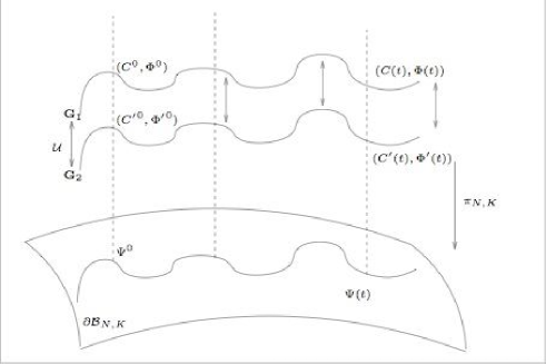
for every (see [28]). A continuous flow on may be lifted by infinitely many continuous flows foliating the fibers that are related by the transitive action of a continuous family of unitary transforms. So called gauge transforms allow then to pass from one flow to another (equivalent) flow such that . This is illustrated on Figure 1 below.
One choice of gauge amounts to imposing
| (3.3) |
to the time-dependent orbitals. Formally the minimization problem (3.2) under the constraints , along with (3.3) leads to the following system of coupled differential equations
for a given initial data in . This system will be referred to as the variational system in the following.
The operator in denotes the projector onto the space spanned by the s. More precisely
| (3.4) |
Actually one checks that
Up to the Lagrange multipliers associated to (3.3) the right-hand side in the variational system corresponds to the Fréchet derivatives of the energy expectation with respect to the conjugate (independent) variables and .
The variational system is well-suited for checking energy conservation and constraints propagation over the flow as shown in Subsection 3.1 below. However it is badly adapted for proving existence of solutions for the Cauchy problem or for designing numerical codes. Equivalent representations of the MCTDHF equations over different fibrations is made rigorous in Subsection 3.3. In particular, we prove below that the variational system is unitarily (or gauge-) equivalent to System (3.26) – named working equations – whose mathematical analysis in the physical case is the aim of Section 4.
Remark 3.1.
Since for every , , the system for the ’s can also be expressed as
| (3.5) |
This equation is then obviously linear in the expansion coefficients. Furthermore, when the ’s (or equivalently the ’s) are kept constant in time, (3.5) is nothing but a Galerkin approximation to the exact Schrödinger equation (1.2). The MCTDHF approximation then reveals as a generalization to a combination of time-dependent basis functions (with extra degree of freedom in the basis functions) of the Galerkin approximation.
3.1. Conservation Laws
In this subsection, we assume the full-rank assumption on the time interval ; that is is invertible for every . We check here that the expected conservation laws (propagation of constraints, conservation of the energy) are granted by the variational system. Recall that to avoid technicalities all calculations in this section are formal but would be rigorous for regular classical solutions. We start with the following
Lemma 3.2 (The dynamics preserves ).
Let being the initial data. If there exists a solution to the system on such that for all , then
Proof.
First we prove that for all . By taking the scalar product of the differential equation satisfied by in with itself, we get
thanks to the self-adjointness of , where and denote respectively real and imaginary parts of a complex number. From the other hand, the full-rank assumption allows to reformulate the second equation in () as
| (3.6) |
(Notice that commutes with .) By definition projects on the orthogonal subspace of , therefore lives in for all . Hence,
| (3.7) |
for all and for all . This achieves the proof of the lemma. ∎
We now check that solutions to the variational system indeed agree with the Dirac-Frenkel variational principle.
Proposition 3.3 (Link with the Dirac-Frenkel variational principle).
Let be a classical solution to on . Then, satisfies the Dirac–Frenkel variational principle (3.1).
Proof.
We start with the characterization (2.33) of the elements in . Since the full-rank assumption is satisfied on , the orbitals satisfy (3.6), and therefore for all and . Firstly, being given , we have
| (3.8) | ||||
thanks to the equation satisfied by . Indeed,
and therefore the sum in (3.8) vanishes thanks to Lemma 2.9. Secondly, for every and for any function in , we have
| (3.9) | ||||
| (3.10) |
Indeed, on the one hand, in virtue of Lemma 2.9, the first term in the right-hand side of (3.9) vanishes whereas the second one identifies with since and both belong to . On the other hand, the last line (3.10) is obtained using the equation satisfied by in and by observing that since . The proof is complete. ∎
Let us now recall the definition of the energy
It is clear that depends on time via . As a corollary to Proposition 3.3 we have the following
Corollary 3.4 (Energy is conserved by the flow).
Let be a solution to on such that lies in the domain of (or in the “form domain” when is semi-bounded) for all in . Then,
3.2. An a posteriori error estimate
We establish an error bound in for the MCTDHF approximation compared with the exact solution to the linear TDSE (1.2). Let us introduce the projection onto the tangent space to at . Then, we claim
Lemma 3.5.
Given an initial data and an exact solution to the -particle Schrödinger equation (1.2). Then, as long as is a solution to in , we have for and the estimate:
Proof.
First, Proposition 3.3 expresses the fact that . Therefore the equation satisfied by the ansatz is:
| (3.12) |
since lives in the tangent space . Next, subtracting (3.12) from (1.2), we get
| (3.13) |
Then, we apply the PDE above to and we integrate formally over . The result follows by taking the imaginary of both sides and by using the self-adjointness of . ∎
Roughly speaking, the above lemma tells that the closer is to the tangent space , the better is the MCTDHF approximation. Intuitively, this is true for large values of . Let us mention that this bound was already obtained in [28] and it is probably far from being accurate. However if the MCTDHF algorithm is applied to a discrete model say of dimension then for large enough ( ) this algorithm coincides with the original problem (see Subsection 7.3).
3.3. Unitary Group Action on the Flow
The variational system is taylor-made for checking energy conservation and constraints propagation over the flow. However it is badly adapted for proving existence of solutions for the Cauchy problem or for designing numerical codes. It is therefore convenient to have at our disposal several explicit and equivalent representations of the MCTDHF equations over different foliations and to understand how they are related. This is the purpose of this subsection. Proofs of technical lemma and theorems are postponed in the Appendix to facilitate straight reading. We start with the following (straightforward) lemma on regular flows of unitary transforms :
Lemma 3.6 (Flow of unitary transforms).
Let and let be in with . Then, defines a continuous family of hermitian matrices, and for all , is the unique solution to the Cauchy problem
| (3.14) |
Conversely, if is a continuous family of Hermitian matrices and if is given, then (3.14) defines a unique family of unitary matrices.
The corresponding flow for unitary transforms on expansion coefficients is as follows:
Corollary 3.7.
The proof of this corollary is postponed to the Appendix. The main result of this section is :
Theorem 3.8 (Flow of unitary equivalent foliations).
Let and . (i) Let be a continuous family of Hermitian matrices on and let be the corresponding solution to (3.14). Assume that there exists a solution of with initial data . Then, the couple with defined by (2.22) and (2.20) is solution to the system
| (3.17) |
with , being defined by (2.22) and with
where is the Hermitian matrix with entries given by (3.16).
Remark 3.9 (Link with Lagrangian interpretation).
The equations can be derived (at least formally) thanks to the Lagrangian formulation: One writes the stationarity condition for the action
over functions that move on . The associated time-dependent Euler–Lagrange equations take the form (3.17) with , an hermitian matrix and with be the hermitian matrix linked to through Eqn. (3.16) above. As observed already by Cancès and Le Bris [8], even if they appear so, the Hermitian matrices and should not be interpreted as time-dependent Lagrange multipliers associated to the constraints since the constraints on the coefficients and the orbitals are automatically propagated by the dynamics (see Lemma 3.15), but rather as degrees of freedom within the fiber at In particular, this gauge invariance can be used to set and to zero for all as observed in Lemma 3.8 and Eqn. (3.23) below, so that the above system can be transformed into the simpler system () we started from.
As a first example of the change of gauge one can use the unitary transforms to diagonalize the matrix for all time and therefore derive the evolution equations for natural orbitals following [5]
Lemma 3.10 (Diagonal density matrix).
Let satisfying with initial data and let that diagonalizes . We assume that for all time the eigenvalues of are simple, that is for and . Define a Hermitian matrix by
and consider the family that satisfies (3.14) with . Then is solution to
with the notation of Theorem 3.8. In particular, for every .
Proof.
As a second application of Theorem 3.8 we investigate particular (stationary) solutions or standing waves. A standing wave for the exact Schrödinger equation is of the form with In the same spirit we look for solutions of System (3.17) with , where is fixed, independent of time, and . Using the formulas (2.29) and (2.30) for the changes of variables, we arrive at
In the above system and are independent of time and is invertible. We start with the equation satisfied by . Observing that the left-hand side lives in whereas the right-hand side lives in , we conclude that there are both equal to zero. Therefore, there exists a matrix that is independent of and such that
| (3.18) |
Also since the left-hand side has to be independent of we get
Comparing now with the equation for the coefficients we infer from Corollary 3.7 that
hence
| (3.19) |
Equations (3.18) and (3.19) are precisely the MCHF equations that are satisfied by critical points of the energy. They were derived by Lewin [26] in the Coulomb case. The real is the Lagrange multiplier corresponding to the constraint whereas the Hermitian matrix is the matrix of Lagrange multipliers corresponding to the orthonormality constraints on the orbitals. Existence of such solutions in physical case is recalled in Section 4. The proof of Theorem 3.13 is postponed in the Appendix and we rather state before some corollaries or remarks. In Physics’ literature the MCTDHF equations are derived from the variational principle (3.1) under the constraints along with additional constraints on the time-dependent orbitals
| (3.20) |
In the above equation is an arbitrary self-adjoint operator on possibly time-dependent named the gauge. In this spirit the variational system corresponds to . Therefore a gauge field is chosen a priori and the corresponding equations are derived accordingly. Both approaches are equivalent by observing that, to every Hermitian matrix , one can associate a self-adjoint operator in such that by demanding that
Conversely being given the family in Theorem 3.13 it follows immediately from the system (3.17) that for all ,
provided is invertible on . We state below Theorem 3.8 that is the equivalent formulation of Theorem 3.13 in terms of gauge. It is based on above remarks together with the following :
Lemma 3.11.
Let be a family of self-adjoint operators on and let such that such that is continuous on Then the matrix with entries is Hermitian and the Cauchy problem (3.14) defines a globally well-defined flow on the set of unitary matrices. In that case, the unitary transforms solve the Cauchy problem (3.15) with in (3.16) given by
| (3.21) |
Remark 3.12.
In Lemma 3.11 the functions are continuous with values in the domain of . When is bounded from below it is enough to assume continuity in the form-domain. When is the Laplace operator or, more generally a one-body time-independent Schrödinger operator, we simply assume that or when is a bounded domain. (Other boundary conditions could of course be considered.)
Theorem 3.13 (Flow in different gauge).
Let , and let be a family of self-adjoint operators in . Assume that there exists a solution to with initial data such that is continuous on for every . Define the family of unitary transforms that satisfy (3.14) with as in Lemma 3.11. Then the couple with defined by (2.22) and (2.20) is a solution to
with , being defined by (2.22) and with being the Hermitian matrix given by (3.16).
Remark 3.14.
Passing from to amounts to change the operator by in both equations and by adding the linear term in the equation satisfied by . Note that whereas solutions to in satisfy
for all , solutions to () satisfy
| (3.22) |
System corresponds to the choice of gauge
This is illustrated and and summarized on Figure 1 below.
Theorem 3.13 and Lemma 3.11 provide with the differential equation that satisfies the unitary matrix that transforms into . A direct calculation shows that, given two self-adjoint one-particle operators and , the solution to
| (3.23) |
with maps a solution to to a solution to . In particular, if we prove existence of solutions for the system for some operator then we have existence of solutions for any system .
Another immediate though crucial consequence of Theorem 3.13 and Theorem 3.8 is given in Corollary 3.15 below. It states that for any choice of gauge the constraints on the expansion coefficients and on the orbitals are propagated by the flow and the energy is kept constant since it is the case for the system . Also the rank of the first-order density matrices does not depend on the gauge.
Corollary 3.15 (Gauge transforms and conservation properties).
Let . Let be a self-adjoint (possibly time-dependent) operator acting on . Assume that there exists a solution to the system on such that and such that the matrix is continuous. Then, for all ,
and the energy is conserved, that is
In addition, satisfies the Dirac-Frenkel variational principle (3.1).
Proof of Corollary 3.15. By Theorem 3.13 and its remark, if satisfies with initial data in , there exists a family of unitary transforms such that where satisfies with same initial data. Since by Lemma 3.2, preserves , so does since and are unitary. Then, by Lemma 2.5, , and the energy is conserved by the flow since it only depends on . Eventually Eqn. (3.1) is satisfied since only depends on the point on the basis and not on the pre-images in the fiber .
So far we have considered a generic Hamiltonian and we have written down an abstract coupled system of evolution equations for this operator. In the following subsection we turn to the particular physical case of -body Schrödinger-type operators with pairwise interactions
3.4. -body Schrödinger type operators with pairwise interactions
At this point, we consider an Hamiltonian in of the following form
| (3.24) |
In the above definition, is a self-adjoint operator acting on . To fix ideas we take . is a real-valued potential, and we denote
Expanding the expression of in the system and arguing as in the proof of Theorem 3.13 we obtain
| (3.25) |
Comparing with System in Theorem 3.13, one observes that the choice of gauge leads to the equivalent system
| (3.26) |
(provided makes sense). From Corollary 3.15 we know that if the initial data in (3.26) lies in it persists for all time. This property allows to recast System (3.26) in a more tractable way where the equations satisfied by the orbitals form a coupled system of non-linear Schrödinger-type equations. This new system that it is equivalent to System (3.26) as long as the solution lies in will be referred to as working equations following [7, 24]. It is better adapted for well-posedness analysis as will be seen in the forthcoming section.
Proposition 3.16 (Working equations).
Let be a solution to (3.26) in , then it is a solution to
| (3.27) |
where (resp. ) is a (resp. ) Hermitian matrix with entries
| (3.28) |
and
| (3.29) |
where here and below we denote
and with the coefficients being defined by (2.10) in Proposition 2.3. Conversely, any solution to (3.27) defines a flow on as long as is invertible and is therefore a solution to (3.26).
Proof.
We have to show that for in
| (3.30) |
and
| (3.31) |
We start from
with
according to (2.9). Since only the coefficients depend on through Eqn. (2.10) we first get
Hence (3.28) by using again Formula (2.10). We now turn to the proof of (3.31) starting from
Then, for every
by interchanging the rôle played by and in the first sum and by using and renaming as in the second one. Comparing with (3.29) we find
To achieve the proof of the proposition we now check that the system of equations in (3.27) preserves as long as is invertible. The claim is obvious as regards the orthonormality of the orbitals since is self-adjoint and since projects on . On the other hand, the equation on the coefficients leads to
since the matrix is Hermitian. ∎
We treat apart in the last two subsections the special cases of the linear free system with no pairwise interaction and of the time-dependent Hartree–Fock equations for the evolution of a single-determinant (TDHF in short) with pairwise interaction.
3.5. Interactionless Systems
In this section we consider systems for which the binary interaction potential is switched off. Then the system (3.26) becomes
From the first equation the coefficients ’s are constant during the evolution. In particular the full-rank assumption is satisfied for all time whenever it is satisfied at start. In the latter case the orbitals satisfy independent linear Schrödinger equations
| (3.32) |
and the -particle wave-function solves the exact Schrödinger equation
| (3.33) |
Conversely, the unique solution to the Cauchy problem (3.33) with coincides with where is the solution to (3.32). This is a direct consequence of the fact that the linear structure of (3.33) propagates the factorization of a Slater determinant. In particular, this enlightens the fact that the propagation of the full-rank assumption is intricately related to the non-linearities created by the interaction potential between particles.
3.6. MCTDHF () contains TDHF
The TDHF equations write (up to a unitary transform)
| (3.34) |
for , with being the self-adjoint operator on that is defined by
The global-in-time existence of solutions in the energy space goes back to Bove, Da Prato and Fano [6] for bounded interaction potentials and to Chadam and Glassey [12] for the Coulomb potentials. They also checked by integrating the equations that the TDHF equations propagate the orthonormality of the orbitals and that the Hartree–Fock energy is preserved by the flow. Derivation of the TDHF equations from the Dirac-Frenkel variational principle may be encountered in standard Physics textbooks (see e.g. [30]). Let us also mention the work [8] by Cancès and Le Bris who have investigated existence of solutions to TDHF equations including time-dependent electric field and that are coupled with nuclear dynamics. By simply setting in the MCTDHF formalism one gets
| (3.35) |
and
for some . In addition according to Remark 2.4,
| (3.36) |
Therefore with the definitions (3.28) and (3.29)
and
Eventually for , according to (3.27), the MCTDHF system in the working form turns out to be
with and Comparing with (3.17), we introduce the Hermitian matrix with entries . According to Lemma 3.6 there exists a unique unitary matrix such that
In virtue of (2.20) the unitary matrix that transforms into is then simply a complex number of modulus () that satisfies
| (3.37) |
Comparing (3.37) with the equation satisfied by in it turns out that . In that special case a change of gauge is simply a multiplication by a global phase factor. Applying Theorem 3.8, the functions , , defined by satisfy the standard Hartree–Fock equations (3.34) and for all time; that is . Being a special case of the MCTDHF setting we then recover “for free” that the TDHF equations propagate the orthonormality of the initial data, that they satisfy the Dirac-Frenkel variational principle and that the flow keeps the energy constant.
4. Mathematical analysis of the MCDTHF Cauchy Problem
This section is devoted to the mathematical analysis of the Cauchy problem for the -body Schrödinger operator with “physical interactions”
| (4.1) |
that is given by (3.26):
In this section . According to Proposition (3.27) solutions to lie in and they are therefore solutions to
| (4.2) |
with
The above system is referred to as the “strong form” of the working equations. Let us emphasize again that it is equivalent to () provided . The main sources of difficulties arise from the fact that the matrix may degenerate and from the Coulomb singularities of the interaction potentials. Our strategy of proof works for more general potentials and . This is discussed in Section 7 below. The spaces and are equipped with the Euclidian norms for the vectors and respectively
Moreover, for a matrix we use the Frobenius norm
We introduce the spaces for endowed with the norms
The main result in this section is the following
Theorem 4.1.
[The MCTDHF equations are well-posed] Let and with in . Then, there exists a maximal existence time (possibly but independent of ) such that:
The global well-posedness in and of the TDHF equations goes back to Chadam and Glassey [12]. Recently Koch and Lubich [24] proved local well-posedness in of the MCTDH and MCTDHF equations for regular pairwise interaction potential and with by using Lie commutators techniques. Our result extends both works. The rest of the section is devoted to the proof of this theorem. The above system with the same notation is rewritten in the “mild form” which makes sense as long as the matrix is not singular:
| (4.3) |
with
| (4.4) |
The strategy of proof is as follows.
In Subsection 4.1 we show that the operator is locally Lipschitz continuous on for in the neighborhood of any point such that is invertible. Observe in particular that is a second-order homogeneous function of the coefficients and therefore the invertibility of this matrix is a local property. Standard theory of evolution equations with locally Lipschitz non-linearities then guarantees local-in-time existence and uniqueness of a mild solution in these spaces that is continuous with respect to the initial data as long as the matrix remains invertible (see e.g [33, 32]). Next for initial data in with , the corresponding mild solution in this space is regular enough to be a strong solution to (4.2) (see [32, 11]). As shown in the previous section (Proposition 3.16), the strong solution then remains on the constraints fiber bundle and it is therefore a solution to (3.26). Furthermore using the gauge equivalence and Corollary 3.15 one deduces that the energy of the solution is conserved and that the Dirac-Frenkel variational principle is satisfied. Recall for further use that the energy may be recasted in the following equivalent forms [17, 26]
| (4.5) |
In consequence for initial data in , , the norm of the vector remains locally bounded in (independently of the norm). Therefore it is also a strong solution in defined on the same time interval which depends only on the norm and on . Eventually using the density of in and the continuous dependence with the initial data one obtains the local-in-time existence of a strong solution in with constant energy.
In Subsection 4.2, relying on the conservation of the energy we prove the existence of the solution over a maximal time interval beyond which the density matrix degenerates. The equations themselves imply the further regularity and
4.1. Properties of the one-parameter group and local Lipschitz properties of the non-linearities
As in Chadam and Glassey [12] for example, one checks that is a one-parameter group of linear operators, unitary in and uniformly bounded in time for in and . We now show that the operator in the right-hand side of (4.3) is a locally bounded and locally Lipschitz continuous mapping in a small enough neighborhood of any in such that is invertible for every . The operator reveals as a composition of locally bounded and locally Lipschitz continuous mappings as now detailed. We first recall that invertible matrices form an open subset of and that the mapping is locally Lipschitz continuous since
In addition, being quadratic, the mapping is for any and independently of locally Lipschitz in in a small enough neighborhood of any such that is invertible. The same holds true for the mapping by composition of locally bounded and locally Lipschitz functions. The operator is a sum of terms of the form with in . Hence, for ,
| (4.6) |
where here and below is a shorthand for a bound with a universal positive constant that only depends on and . Therefore is locally Lipschitz from to since it is quadratic with respect to . To deal with the other non-linearities we start with recalling a few properties of the Coulomb potential taken from [12, Lemma 2.3]. Their proof is a straightforward application of Cauchy–Schwarz’ and Hardy’s inequalities and we skip it. Let , then with , , and we have
| (4.7) |
and
As a consequence of above inequalities and by an induction argument that is detailed in [9] for example, we have, for and for every ,
| (4.8) |
with . First, recall from (3.29), that is a sum of terms of the form with the coefficients depending quadratically on according to (2.10). They are therefore locally Lipschitz continuous with respect to . Gathering with (4.8) we have
| (4.9) |
The mapping is then locally bounded in and being quadratic in and cubic in it is locally Lipschitz continuous in by a standard polarization argument. In particular, the first bounds reveals a linear dependence on the norm. Eventually, for every , using (4.7) and Hölder’s inequality we obtain
the last line being a direct consequence of (4.8). In particular this proves
| (4.10) |
| (4.11) |
and that is locally Lipschitz continuous in since according to (3.28), is a finite sum of terms of this kind up to some universal constant. For any existence and uniqueness of a solution to the integral equation (4.3) in a neighborhood of in for small enough follows by Segal’s Theorem [33], which also ensures the continuity with respect to the initial data in . We now turn to the existence of a maximal solution and to the blow-up alternative in .
4.2. Existence of the maximal solution and blow-up alternative
To simplify notation, from now on we use the shorthand for . Existence of a global-in-time solution requires to control uniformly both the norm of and the norm of . With the conservation of the energy this turns to be equivalent to control only the norm of . Let denotes the maximal existence time and assume that . We first show that
| (4.12) |
We argue by contradiction and assume that there exists a positive constant such that for all , . We now prove that there exists a positive constant such that
| (4.13) |
Thanks to Lemma 3.4 and Corollary 3.15, the energy is preserved by the flow, and therefore using the expression (4.5)
for all since, with ,
for . As in [26, 17], Kato’s inequality then yields that
where is a positive constant independent of . Now let be the smallest eigenvalue of the hermitian matrix . Then according to the definition of the Frobenius norm
with being the eigenvalues of , hence
for all . Therefore
| (4.14) |
In particular, this shows (4.13) with . Therefore, for any arguing as above, we may build a solution to the system on for that only depends on and . Since is arbitrary close to we reach a contradiction with the definition of . Hence (4.12). Now, taking the derivative with respect to of both sides of , we get
| (4.15) |
for all . From the expression of in terms of and since , it holds
in virtue of the bound (4.10) on using the fact that . Inserting the last bound above in (4.15) and integrating over yields
for all . Because of (4.12), this implies that . So far we have proved the local well-posedness of the MCTDHF equations in for every and the existence of a maximal solution in until time when the density matrix becomes singular. We prove now that is the maximal time of existence regardless of the imposed regularity on the solution. Let be a solution in , then it is in particular a maximal solution in . We have to show that the norm of cannot explode at finite time . Indeed, for any , we have
| (4.16) |
by definition of , hence
| (4.17) |
From the Duhamel formula for the PDEs system (4.3)–(4.4) and using the bounds (4.6) and (4.8) together with and , we get for all
where is a positive constant that only depends on the local bounds (4.16) and (4.17). By Gronwall’s lemma we infer
hence the conclusion. The proof for any follows then by a straightforward induction argument using the corresponding bounds (4.6) and (4.8) by assuming that . The proof of Theorem 4.1 is now complete.
4.3. Existence of Standing wave solutions
In the present case the equations for the coefficients write (3.19) while Eqn. (3.18) for the orbitals becomes:
| (4.18) |
according to Proposition 3.16. In [25] Le Bris has proved the existence of ground-states - that is, minima of the energy over the set - for the physical Hamiltonian (1.1), on the whole space , and under the assumptions and . Later on Friesecke extended this result to general admissible pairs , under the same assumption on the nuclear charge. Finally Lewin proved the existence of infinitely many critical points of the MCHF energy for any pairs , hence the existence of infinitely many solutions to the coupled system (4.18) – (3.19) that satisfy the full-rank assumption. All these solutions then give rise to infinitely many standing waves of the MCTDHF system and thereby to particular global-in-time solutions.
The conservation of the invertibility of the matrix being an essential issue in the MCTDHF setting it is natural to give sufficient condition for such property.
5. Sufficient condition for global-in-time existence
In this section we focus again on the -body Schrödinger operator (1.1) with physical interactions (4.1). For any with fixed , we denote
the “- ground state energy”. Obviously one has
| (5.1) |
with being the bottom of the spectrum of on . Recall that the maximal rank hypothesis corresponds to the following equivalent facts :
-
(i)
The rank of the operator is equal to ;
-
(ii)
The matrix is invertible;
-
(iii)
The smallest eigenvalue of is strictly positive.
Since this is satisfied for (Hartree–Fock case) and since must be admissible, we now assume that . The main result of this section is the following:
Theorem 5.1.
Let be an initial data in (3.27) with invertible. Assume that then
As an immediate by-product we get a sufficient condition ensuring the global-in-time invertibility of the matrix .
Corollary 5.2.
If satisfies
| (5.2) |
then ; that is, the maximal solution is global-in-time.
Remark 5.3.
Remark 5.4.
A key difficulty in the proof of above theorem is that the energy functional is not weakly lower semi-continuous in while it is in for any bounded domain as already observed by Friesecke [17]. When is a bounded domain of or when the potential is non-negative, the proof of Theorem 5.1 is much easier thanks to the lower semi-continuity, and it is detailed in [3]. In the general case the proof is in the very spirit of Lewin’s one for the convergence of critical points of the energy functional [26].
Proof of Theorem 5.1. Let be the maximal solution to (3.27) on with initial data given by Theorem 4.1. We assume that , then
Equivalently, with the eigenvalues of being arranged in decreasing order , this means
Then there exists a sequence converging to , a positive number and an integer such that
| (5.3) |
Indeed, since , at least eigenvalues stay away from zero when goes to . We denote , , , and so on for other involved quantities. For all , . Thus according to Proposition 2.5, there exists a unique sequence of unitary transforms that map into with being an eigenbasis for the operator . In particular the corresponding matrix is diagonal. In other words,
Since the group of unitary transforms is compact, we may argue equivalently on the sequence that we keep denoting by for simplicity. From (5.3)
| (5.4) |
Then,
| (5.5) |
for in virtue of (2.12). In particular, the sequence being compact
| (5.6) |
We decompose
with
Then
as a consequence of (5.5) and since each determinant is normalized in . Hence
| (5.7) |
Since the MCTDHF flow keeps the energy constant, we have
for all . This property provides with additional information on the sequence . Using the fact that the ’s diagonalize , the energy (4.5) rewrites
| (5.8) |
where in (5.8) we used the positivity of the two-body interaction potential . By the Kato inequality, for any , there exists such that
in the sense of self-adjoint operators. Then
Therefore, inserting into (5.8),
Thus, for all , is bounded in . Then, from (5.4) and extracting subsequences if necessary, we obtain the alternative
| (5.9) |
and
| (5.10) |
Since, under the hypotheses on , the map is weakly lower semi-continuous on , we deduce from (5.9) that
| (5.11) |
We now check that
| (5.12) |
by showing that
| (5.13) |
Let . We assume without loss of completeness that . From the expression (2.10) for , we observe that
| (5.14) |
since . We thus get
| (5.15) |
from (5.4). Then thanks to (4.7) and (5.14)
since the norms of the orbitals equal and since in any case is bounded in independently of . Therefore each term which appears in the sum in (5.13) converges to as goes to infinity thanks to (5.9). Claim (5.13) then follows. Gathering together (5.11) and (5.12) we have
| (5.16) | |||||
The point now consists in showing that the right-hand side in (5.16) is bounded from below by . Indeed, let us set where and . There is a slight difficulty arising here from the fact that (with obvious notation) is close but different from and similarly for and . (Also is not normalized in (only asymptotically) but this will be dealt with afterwards.) First we observe that because of (2.11) for every ,
goes to as goes to infinity thanks to (5.5). In addition, each term of the form is bounded independently of for . Therefore
| (5.17) |
For the same reason, and with obvious notation, for all ,
since according to (2.10) the extra terms in these differences only involve coefficients with . Again each term of the form is bounded independently of for . Therefore
| (5.18) |
Therefore, gathering together (5.16), (5.17) and (5.18),
| (5.19) |
Since is not in (it is only the case asymptotically), is not in , thus we cannot bound immediately from below by . Anyway, in virtue of (5.6),
| (5.20) |
The energy being quadratic with respect to
| (5.21) |
for for all . Gathering together (5.19), (5.20) and (5.21) and taking the limit as goes to infinity we deduce
| (5.22) |
Hence the theorem.
Remark 5.5.
When is a bounded domain of , any sequence in is relatively compact in thanks to the Rellich theorem. On the other hand, the energy functional is weakly lower semi-continuous in . Therefore it is easily checked in that case that
with being the weak limit of the sequence introduced in the above proof.
Remark 5.6 (Stability, Consistency and Invertibility of the density matrix ).
The main factor in the instability of the working equations or any gauge-equivalent system, is the inverse of the density matrix. In the present section, criteria for the global invertibility of have been given. These criteria do not provide with an uniform estimate for , and furthermore increasing the consistency of the MCTDHF approximation leads to an increase of the number of orbitals. As usual consistency and stability are both necessary and antinomic. Indeed, the most obvious observation is that one always has
for has at most positive eigenvalues whose sum equals . Therefore the smallest can be at most . These considerations lead either to a limitation on or to a regularization or a “cut-off” of . In fact the “consistency” in the sense of numerical analysis is obtained with fixed by letting go to infinity. This is basically different from the idea (in spirit of statistical mechanics) of letting go to infinity [4].
6. Stabilization of and existence of solutions
In the above analysis, both for existence of maximal solutions and for global invertibility of the density matrix, the conservation of energy plays a crucial rôle. Besides the theoretical interest, the analysis of an MCTDHF system with infinite (or non conserved) energy but finite mass is relevant. Indeed, to circumvent the possible degeneracy of the density matrix, physicists resort to ad hoc methods like perturbations of this matrix in order to ensure its invertibility. Typically, this is achieved as follows
| (6.1) |
(see e.g. [7]), or by taking
| (6.2) |
for small values of (see [5]). Note that in latter case vanishing eigenvalues are perturbed at order while the others are unchanged up to exponentially small errors in terms of . Then the perturbed system reads for an
| (6.3) |
On the other hand, when a laser field is turned on, the Hamiltonian of the system is then time-dependent which is a relevant configuration from the physical point of view (see [7] and Section 7 below). In such situation, the conservation of the energy fails and a recourse to alternative theories is necessary.
However in both situations the norm (which corresponds to the electronic charge) is conserved and this justifies an analysis of the MCTDHF outside the energy space. Therefore the Strichartz estimates turn out to be a natural tool in the same spirit as Castella [9] and Zagatti [36]. In [31], existence and uniqueness of global-in-time mild solutions has been obtained for initial data. As in the previous section (and with the same notation) the perturbed working equations are written in “Duhamel” form
where denotes the group of isometries generated by on . The potentials and belong to
From the relation
and
one deduce by interpolation the so-called Strichartz estimates
that hold for any Strichartz pairs with . (Strichartz estimates for the endpoints and are more intricate and due to Keel and Tao [22]).
Following Zagatti [36] and Castella [9], the spaces
are introduced for any Strichartz pairs. For some and some small enough, the non-linear operator which appears in the Duhamel integral
is a strict contraction in the ball
Next using the conservation of the norms of the orbitals and the estimate
one follows the lines of Tsutsumi in [35] to get existence and uniqueness of a strong solution in (see the details in [31]). This is summarized in the
Proposition 6.1.
Let . For any initial data and for any Strichartz pairs , the -regularized working equations admit a unique strong solution
that lives in for all . If in addition then .
Eventually one expects that whenever the original solution is well-defined (with a non degenerate density matrix ) on a time interval it will be on the same interval the limit for of the solution of the perturbed working equations. This is the object of the following
Theorem 6.2.
Proof.
We first recall the obvious a posteriori bounds
on , and, as a consequence of (6.4) and the energy conservation,
with . We can also rely on the orthonormality of the orbitals in and . We introduce the notation
where
and where the index means that the claim holds both for the regularized system and the initial one, uniformly in . System (6.3) can also be written in synthetic form:
| (6.5) | ||||
| (6.6) |
Since the initial is in and since the regularized system propagates the regularity, is in for all time. We fix . We introduce a parameter to be made precise later and the set
with . The mappings being continuous from to , the set is closed and since , there exists a maximal time in such that
We now prove by contradiction that . Assume then . Subtracting (6.5) to (6.6) and taking norms first yields to
| (6.7) |
for all . Here and below denotes a positive constant that may vary from line to line but that is independent of and continuous and non-decreasing with respect to . Indeed we use the fact that the non-linearity is locally Lipschitz continuous in (Subsection 4.1) together with the uniform bound
On the other hand, we write
| (6.8) |
by using the local Lipschitz bounds of given in Subsection 4.1. We now turn to the quantity . Both regularization (6.1) and (6.2) of the density matrix take the form :
with . Then,
| (6.9) |
by using the obvious bound for , where only depends on and . We now assume that
| (6.10) |
where is given in the statement of the theorem. Using
we deduce
Therefore
by using (6.9). Hence
| (6.11) |
since by (6.10) and for in . Inserting (6.11) in (6.8) we get:
| (6.12) |
Eqn. (6.12) together with (6.7) finally leads to
| (6.13) |
for all . Eventually, thanks to Gronwall’s inequality,
| (6.14) |
With as in (6.10), next
| (6.15) |
we get
By continuity of , we may then find such that . Hence the contradiction with the definition of . Therefore, and, going back to (6.14) we obtain:
| (6.16) |
for say and small enough, satisfying (6.15), whence the result. ∎
In the forthcoming (and last) section we comment on straight extensions of the above analysis.
7. Extensions
The present contribution is focused on the algebraic and functional analysis properties of the MCTDHF equations for fermions. Multi-configuration approximations can also be considered for symmetric wave-functions or also for wave-functions with no symmetry (see e.g. [5, 24]). The mathematical analysis of the equations which play the rôle of the “working equations” of Section 3 is similar. On the other hand, the fermionic case is important by itself and leads to much better geometric structure in terms of principal fiber bundle as described in Section 2. Hence our choice. Our results could be generalized to general (symmetric) -body interactions as well including the -body density matrices.
7.1. Beyond Coulomb potentials.
Although above results and proofs are mainly detailed for Coulomb potentials they carry through more general real-valued potentials. Indeed well-posedness results in and are still valid for and in the class with , and . These conditions ensure that is self-adjoint in , that the one-body operator is a semi-bounded self-adjoint in with domain and that the Kato inequality holds for the potential . Under these assumptions, the energy space is (respectively when is a bounded domain) and the propagator is a one-parameter group of unitary operators in and in .
For the global well-posedness sufficient condition to hold true (Theorem 5.1 and its corollary) further conditions on the potentials are required to ensure that the energy functional is weakly lower semi-continuous on the energy space. Sufficient conditions are (for example) or (the negative part of ) tending to at infinity at least in a weak sense.
7.2. Extension to time-dependent potentials.
One of the basic use of the MCTDHF is the simulation of ultra-short light pulses with matter [37]. Describing this situation leads to the same type of equations but with the one-body Hamiltonian being replaced by a one-body time dependent hamiltonian
with and real, and as in the above subsection. A typical example is for some positive real parameters , and [37, 38]. This does not change neither the algebraic and geometrical structure of the equations nor the definition of the density matrix nor the notion of full-rank. The potential vector being independent of the variable the energy space is . With convenient hypotheses (say and continuous, bounded with bounded derivatives), the results in Section 4 concerning local-in-time well-posedness of the Cauchy problem remain valid. For generalization of the use of Strichartz estimates and the local well-posedness one should follow for example [10]. Since the energy is now time-dependent extra hypothesis have to be introduced for the persistence of the full-rank assumption done in Section 5.
Assume that and take their values in a bounded set (the set of “control” ) and that their derivatives are also bounded. The system (3.25) with replaced by keeps on preserving the constraints since Lemma 3.2 only relies on the self-adjointness of the Hamiltonian. Similarly solutions to (3.25) satisfy the Dirac–Frenkel variational principle. The energy is no longer conserved by the flow. Indeed, following the lines of the proof of Corollary 3.4, we have
with the prime denoting time derivatives. However
and the energy in controlled for any finite time, whence the existence of a maximal solutions in as long as the matrix remains invertible.
To adapt the result concerning the global full-rank hypothesis, we introduce the minimization problems for any real numbers and
with
for . The global-in-time conservation of full-rank in Theorem 5.1 remains true under the hypothesis
There is a lot of room for improvement in the above argument. For example, if we assume that, for all time, the solution satisfies
for a given function , then by the Gronwall lemma
The result of Theorem 5.1 remains true provided
7.3. Discrete systems.
The emphasis has been but in particular for the functional analysis on the case when although in the first part we have described the problem in any open subset of . In fact all the formal and algebraic derivations can also be adapted to the case when is a discrete set equipped with a discrete Lebesgue measure and in particular when is a finite set [3].. Such situation is important for two reasons. On the one hand many models of quantum physics (the Ising model for instance) involve a discrete Hamiltonian defined on a discrete set. On the other hand the discretization of the original problem in view of any numerical algorithm leads to a discrete problem.
Up to now only a rough a posteriori error estimate has been proven. However if the MCTDHF algorithm is applied to a discrete model say of dimension then one always has . The error formula (3.13) shows that, for , the MCTDHF algorithm is exact. It should be eventually observed that in general the two operations : - Discretization of the original -particle problem and use of a MCTDHF approximation or - Use of a MCTDHF approximation and then discretization of the equations, lead to different algorithms.
Appendix – Proofs of technical lemmas in Subsection 3.3
Proofs of Corollary 3.7 and Lemma 3.11
For and given and fixed it is convenient to denote by the column vector in with entries and by
the determinant composed with these vectors. With this notation (3.14) gives
| (7.1) |
Differentiating the relation
and using the multi-linearity with respect to the column vectors and Eqn. (7.1) one obtains:
| (7.2) |
On the other hand since is a flow of unitary matrices it is solution to a differential equation of the following type:
| (7.3) |
Identification of the coefficients of
gives, taking in account the number of permutation needed to change
Let us now prove (3.21). Let . We first observe that
| (7.4) |
Now we use (2.5) and the Laplace method to develop a determinant with respect to the row that contains the terms involving to get
in virtue of (2.4). Hence (3.21) using (3.16) and the definition of .
Proofs of Theorem 3.13 and Theorem 3.8.
Let be a solution to and let be as in the statement of the theorem. With we define the family of unitary transforms according to Lemma 3.11 and is then given by Corollary 3.7. We set , and . Thanks to (3.15), solves
| (7.5) |
Then, for all ,
thanks to (2.29) and (7.5). On the one hand, since is unitary,
On the other hand, when is obtained through , we get by a direct calculation from (3.21)
Combining these two facts we get the first equation in , namely
We turn now to the equation satisfied by . To simplify the notation we use the shorthand for and for respectively. Then, using and (3.14), we have
| (7.6) |
thanks to (2.30) and since clearly for . It is easily checked that when is given through we have
and therefore
Hence (7.6) also writes
We now check that, for all ,
thereby proving that
Indeed, for all , using (2.32) in Lemma 2.9 in (7.7) and using (7.4) in (7.8), we have
| (7.7) | ||||
| (7.8) | ||||
by the definition (2.28) of ; whence the result since is arbitrary in .
Acknowledgment
This work was supported by the Austrian Science Foundation (FWF) via the Wissenschaftkolleg “Differential equations” (W17), by the Wiener Wissenschaftsfonds (WWTF project MA 45) and the EU funded Marie Curie Early Stage Training Site DEASE (MEST-CT-2005-021122). The authors warmly acknowledge Mathieu Lewin for a careful reading of a preliminary version of this work and for his valuable comments. They also would like to thank Alex Gottlieb for many discussions and suggestions.
References
- [1] T. Ando, Properties of Fermions Density Matrices, Rev. Modern Phys. 35 (3), 690–702 (1963).
- [2] A. Baltuska, Th. Udem, M. Uiberacker, M. Hentschel, Ch. Gohle and R. Holzwarth, V. Yakovlev, A. Scrinzi, T. W. Hänsch, and F. Krausz. Attosecond control of electronic processes by intense light fields, Nature 421, 611 (2003).
- [3] C. Bardos, I. Catto, N.J. Mauser and S. Trabelsi, Global-in-time existence of solutions to the multi-configuration time-dependent Hartree-Fock equations: A sufficient condition. Applied Mathematics Letters 22, 147–152 (2009)
- [4] C. Bardos, F. Golse, N.J. Mauser and A. Gottlieb, Mean-field dynamics of fermions and the time-dependent Hartree–Fock equation. J. Math. Pures et Appl. 82, 665–683 (2003)
- [5] M. Beck, A. H. Jäckle, G.A. Worth and H. -D. Meyer, The multi-configuration time-dependent Hartree (MCTDH) method: a highly efficient algorithm for propagation wave-packets. Phys. Rep. 324, 1–105 (2000)
- [6] A. Bove, G. Da Prato and G. Fano, On the Hartree-Fock time-dependent problem. Comm. Math. Phys. 49, 25–33 (1976)
- [7] J. Caillat, J. Zanghellini, M. Kitzler, O. Koch, W. Kreuzer and A. Scrinzi, Correlated multi-electron systems in strong laser fields – An MCTDHF approach. Phys. Rev. A 71, 012712 (2005)
- [8] E. Cancès and C. Le Bris, On the time-dependent Hartree–Fock equations coupled with a classical nuclear dynamics. Math. Models Methods Appl. Sci. 9, 963–990 (1999).
- [9] F. Castella, solutions to the Schrödinger–Poisson system: existence, uniqueness, time behavior, and smoothing effects. Math. Models Methods Appl. Sci. 7 (8), 1051–1083 (1997).
- [10] T. Cazenave, An introduction to nonlinear Schrödinger equations, Second Edition, Textos de Métodos Mathemáticas 26, Universidade Federal do Rio de Janeiro (1993).
- [11] T. Cazenave and A. Haraux, An introduction to semi-linear evolution equations. Oxford Lecture Series in Mathematics and Its Applications 13, Oxford University Press, New York, 1998.
- [12] J.M. Chadam and R.T. Glassey, Global existence of solutions to the Cauchy problem for the time-dependent Hartree equation. J. Math. Phys. 16, 1122–1230 (1975)
- [13] A.J. Coleman, Structure of Fermion Density Matrices. Rev. Mod. Phys. 35(3), 668–689 (1963)
- [14] A.J. Coleman and V.I. Yukalov, Reduced Density Matrices: Coulson’s Challenge, Lectures Notes in Chemistry 72, Springer-Verlag Berlin Heidelberg (2000)
- [15] P. A. M. Dirac, Proc. Cambridge Phil. Soc 26, 376 (1930)
- [16] J. Frenkel, Wave Mechanics, Oxford University Press, Oxford (1934)
- [17] G. Friesecke, The multi-configuration equations for atoms and molecules: charge quantization and existence of solutions. Arch. Rational Mech. Anal. 169, 35–71 (2003)
- [18] G. Friesecke, On the infinitude of non-zero eigenvalues of the single-electron density matrix for atoms and molecules. R. Soc. Lond. Proc. Ser. A Math. Phys. Eng. Sci. 459(2029), 47–52 (2003)
- [19] A.D. Gottlieb and N.J. Mauser, Properties of non-freeness: an entropy measure of electron correlation, Int. J. of Quantum Information 5(6), 10–33 (2007). E–print arXiv:quant-ph/0608171v3.
- [20] R. Grobe, K. Rza̧żewski and J. H. Eberly, Measure of electron-electron correlation in atomic physics. J. Phys. B. 27, L503–L508 (1994).
- [21] T. Kato and H. Kono, Time-dependent multi-configuration theory for electronic dynamics of molecules in an intense laser field. Chem. Phys. Lett. 392, 533–540 (2004).
- [22] M. Keel and T. Tao, Endpoint Strichartz estimates. Am. J. Math. 120, 955–980 (1998).
- [23] O. Koch, W. Kreuzer and A. Scrinzi, Approximation of the Time-Dependent Electronic Schrödinger Equation by MCTDHF. Appl. Math. Comput. 173, 960–976 (2006).
- [24] O. Koch and C. Lubich, Regularity of the Multi-Configuration Time-Dependent Hartree Approximation in Quantum Molecular Dynamics. M2AN Math. Model. Numer. Anal. 41, 315–331 (2007).
- [25] C. Le Bris, A general approach for multi-configuration methods in quantum molecular chemistry. Ann. Inst. H. Poincaré Anal. Non Linéaire 11(4), 441–484 (1994).
- [26] M. Lewin, Solutions of the Multi-configuration Equations in Quantum Chemistry. Arch. Rational Mech. Anal. 171(1), 83–114 (2004).
- [27] P.O. Löwdin, Quantum Theory of Many-Particles Systems, I: Physical Interpretations by Mean of Density Matrices, Natural Spin-Orbitals, and Convergence Problems in the Method of Configurational Interaction. Phys. Rev. 97, 1474–1489 (1955).
- [28] C. Lubich, On variational approximations in quantum molecular dynamics. Math. Comp. 74, 765–779 (2005).
- [29] C. Lubich, A variational splitting integrator for quantum molecular dynamics. Appl. Numer. Math. 48, 355–368 (2004).
- [30] R. McWeeny, Methods of molecular quantum mechanics, 2nd ed., Academic Press, 1992.
- [31] N.J. Mauser and S. Trabelsi, analysis of the Multi-configuration Time-Dependent Equations. Submitted.
- [32] A. Pazy, Semi-groups of linear operators and applications to partial differential equations. Springer-Verlag, Berlin, 1983.
- [33] I. Segal, Non-linear semi-groups. Annals of Mathematics 78, 339–364 (1963)
- [34] S. Trabelsi, Solutions of the Multi-configuration Time-Dependent Equations in Quantum Chemistry. C. R. Math. Acad. Sci. Paris 345(3), 145–150 (2007).
- [35] Y. Tsutsumi, Solutions for nonlinear Schrödinger Equation and Nonlinear Groups. it Funk. Ekva. 30, 115–125 (1987)
- [36] S. Zagatti, The Cauchy problem for Hartree–Fock time dependent equations. Ann. Inst. H. Poincaré, Phys. Th. 56(4), 357–374 (1992).
- [37] J. Zanghellini, M. Kitzler, C. Fabian, T. Brabec and A. Scrinzi, An MCTDHF approach to multi-electron dynamics in laser fields. Laser Physics 13 (8), 1064–1068 (2003).
- [38] J. Zanghellini, M. Kitzler, T. Brabec and A. Scrinzi, Testing the multi-configuration time-dependent Hartree-Fock method. J. Phys. B: At. Mol. Phys. 37, 763–773 (2004).