Cluster formation and the Sunyaev-Zel’dovich power spectrum in modified gravity: the case of a phenomenologically extended DGP model

Abstract

We investigate the effect of modified gravity on cluster abundance and the Sunyaev-Zel’dovich angular power spectrum. Our modified gravity is based on a phenomenological extension of the Dvali-Gabadadze-Porrati model which includes two free parameters characterizing deviation from $\Lambda$CDM cosmology. Assuming that Birkhoff’s theorem gives a reasonable approximation, we study the spherical collapse model of structure formation and show that while the growth function changes to some extent, modified gravity gives rise to no significant change in the linear density contrast at collapse time. The growth function is enhanced in the so called normal branch, while in the “self-accelerating” branch it is suppressed. The Sunyaev-Zel’dovich angular power spectrum is computed in the normal branch, which allows us to put observational constraints on the parameters of the modified gravity model using small scale CMB observation data.

1 Introduction

General Relativity is surely the most successful theory of gravity that passes accurate tests in the solar system and laboratories. However, current cosmological observations indicate the presence of dark matter and dark energy; a large fraction of the Universe is made of unknown components. The mystery of the dark components is based on general relativity, and hence it tells us that what we do not know may be the long distance behaviour of gravity rather than the energy-momentum components in the Universe. In this sense, cosmological observations open up a new window to study the properties of gravity on large scales.

There are various alternative theories of gravity leading to interesting cosmological consequences. For example, the Dvali-Gabadadze-Porrati (DGP) model (Dvali et al., 2000) is one of the extra dimensional scenarios that can account for cosmic acceleration without introducing dark energy. The $f(R)$ theories, which modify the four-dimensional Einstein-Hilbert action explicitly, also realise the accelerated expansion of the Universe (Sotiriou & Faraoni, 2008). MOND (Milgrom, 1983) and its relativistic extension (Bekenstein, 2004) explain galactic rotation curves without need for dark matter. A more phenomenological way of changing gravity is to assume Yukawa-like modification to a gravitational potential. Such modification yields effectively a scale-dependent Newtonian constant, and its effect on the evolution of large scale structure has been investigated (Sealfon et al., 2005; Shirata et al., 2005; Shirata et al., 2007; Stabenau & Jain, 2006; Martino et al., 2008).

One of the powerful ways for distinguishing modified gravity from the $\Lambda$CDM model is to study the growth function because the modified growth function would leave its footprints on the cosmological large-scale structure. In this context, many authors have studied the integrated Sachs-Wolfe effect and weak lensing in modified gravity, and obtained observational constraints on modified gravity models. For instance, Schmidt (2008) investigated the effect of $f(R)$ gravity, the DGP model, and tensor-vector-scalar theory on weak lensing, and showed that for detecting signatures of modified gravity the weak lensing observation is a better probe than the integrated Sachs-Wolfe effect measured via the galaxy-CMB cross-correlation. Thomas et al. (2008) put constraints on the DGP model by using weak lensing data (CFHTLS-wide) combined with baryon acoustic oscillations and supernovae data. Schmidt et al. (2009) have studied the statistical properties of dark halos in $f(R)$ gravity by employing numerical simulations.

In this paper, we consider a generalisation of the DGP model, adding a term $\pm H^{2\alpha}/r_{c}^{2(1-\alpha)}$ in the Friedmann equation, where $\alpha$ and $r_{c}$ are the model parameters (Dvali & Turner, 2003; Koyama, 2006; Afshordi et al., 2008; Khoury & Wyman, 2009). The generalised model reduces to the self-accelerating and normal branches of the DGP model (with a cosmological constant) by taking $\alpha\to 1/2$, and reproduces the $\Lambda$CDM model in the $\alpha\to 0$ limit. Afshordi et al. (2008) studied cosmological perturbations in this modified gravity theory under several assumptions, and discussed various observational consequences of the model. Khoury & Wyman (2009) performed N-body simulations in the same model recently. We shall work on a different approach in the present paper: assuming that Birkhoff’s theorem gives a reasonable approximation (as implied by Koyama (2006)), we study the spherical collapse model of structure formation with the modified Friedmann equation. Using the spherical collapse scenario, we can compute the Sunyaev-Zel’dovich (SZ) angular power spectrum through the Press-Schechter formalism (Press & Schechter, 1974). Since the SZ angular power spectrum is sensitive to the distribution of dark halos, it is a good probe of modified distribution of dark halos in the generalised DGP model.

Before closing the introduction we should note that in any case modified gravity must satisfy solar system and laboratory tests, and some $f(R)$ models and the original DGP model indeed have mechanisms to reproduce ordinary gravity around the Sun and on the Earth. This point is not clear in the present model and is beyond the scope of the paper. We only remark that our Friedmann equation reduces to the ordinary one at high densities.

This paper is organized as follows. In the next section, we describe our modified gravity model in terms of the Friedmann equation and explain its possible origin. In Sec. 3, we review the spherical collapse model of structure formation in modified gravity, and compute the linear growth function and the linear density contrast at collapse time. Then, in Sec. 4, we study the effect of modified gravity on the SZ angular power spectrum. Observational constraints on the model parameters are discussed. Finally, we conclude in Sec. 5.

2 The model

The DGP braneworld was originally proposed as a model for recovering 4D gravity on the brane even in an infinitely large 5D Minkowski bulk (Dvali et al., 2000). In the DGP braneworld, gravity is modified at long distances, while standard 4D gravity is indeed reproduced at short distances (through a complicated nonlinear mechanism – e.g., Tanaka, 2004; Koyama & Silva, 2007; Lue & Starkman, 2003; Lue et al., 2004), so that the model passes solar system and laboratory tests. Probably the most intriguing consequence of the DGP braneworld comes out in the modified Friedmann equation (Deffayet et al., 2002):

$$H^{2}=\frac{8\pi G}{3}\rho\pm\frac{H}{r_{c}}.$$ (1)

Here, $r_{c}$ is the crossover scale above which gravity looks 5D. With the upper (plus) sign and $r_{c}\sim H_{0}^{-1}$ (the present Hubble horizon scale), we have the “self-accelerating” solution which could be the origin of the current cosmic acceleration. In this paper, however, we do not assume that modified gravity is directly responsible for the accelerated expansion.

The model we consider is a phenomenological extension of the DGP braneworld described by the modified Friedmann equation

$$H^{2}=\frac{8\pi G}{3}\rho+\frac{\Lambda}{3}\pm\frac{H^{2\alpha}}{r_{c}^{2(1-\alpha)}},$$ (2)

where $0\leq\alpha<1$. This is similar to the model of Dvali & Turner (2003), but we allow for a different sign of the last term and include the cosmological constant $\Lambda$ explicitly (Afshordi et al., 2008). With the upper (respectively lower) choice of sign we use the terminology the self-accelerating (respectively normal) branch, though it is not self-accelerating in the upper sign case. Equation (2) with $\alpha=1/2$ corresponds to the DGP cosmology (with a cosmological constant or the tension on the brane), while $\alpha=1$ can be absorbed into a redefinition of the gravitational constant $G$. Expansion history of $\Lambda$CDM cosmology is recovered in the limit $\alpha\to 0$.

The modified Friedmann equation (2) can be recast in

$$\left(\frac{H}{H_{0}}\right)^{2}=\frac{\Omega_{{\rm m}0}}{a^{3}}+\lambda\pm(r_{c}H_{0})^{-2(1-\alpha)}\left(\frac{H}{H_{0}}\right)^{2\alpha},$$ (3)

where

$$\lambda:=1-\Omega_{{\rm m}0}\mp(r_{c}H_{0})^{-2(1-\alpha)},$$ (4)

$\Omega_{{\rm m}0}:=8\pi G\rho_{0}/(3H_{0}^{2})$, and the present scale factor is chosen to be $a_{0}=1$. If $\Lambda(\propto\lambda)=0$ and the accelerated expansion were supported by modified gravity in the self-accelerating branch, successful cosmology would require $r_{c}\sim H^{-1}_{0}$. In the present case, however, $\Lambda$ is responsible for the accelerated expansion as in conventional cosmology, and therefore we are in principle allowed to take $r_{c}<H^{-1}_{0}$ (e.g., $r_{c}\sim 0.1H^{-1}_{0}$). In particular, for sufficiently small $\alpha$, expansion history is very close to that in standard $\Lambda$CDM cosmology even if we take relatively small $r_{c}$ (Afshordi et al., 2008). Indeed, for $\alpha=0.1$, $r_{c}H_{0}=0.4$, and $\Omega_{{\rm m}0}=0.26$, the dimensionless physical distance

$$E(a):=H_{0}\int^{1}_{a}\frac{{\rm d}a}{a^{2}H(a)},$$ (5)

differs from the corresponding $\Lambda$CDM result by less than one percent (Fig. 1).

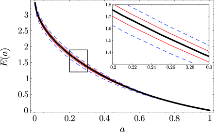
Figure 1: Dimensionless physical distance. Parameters are (from top to bottom): (1) $\alpha=0.1$, $r_{c}H_{0}=0.4$; (2) $\alpha=0.01$, $r_{c}H_{0}=0.2$; (3) $\Lambda$CDM; (4) $\alpha=0.01$, $r_{c}H_{0}=0.2$; (5) $\alpha=0.1$, $r_{c}H_{0}=0.4$. The cases (1) and (2) are for the normal branch and the cases (4) and (5) are for the self-accelerating branch. In all the cases $\Omega_{{\rm m}0}=0.26$.

Unfortunately, we do not have concrete higher dimensional models that account for Eq. (2). One possibility is that such modification could be derived from a higher codimension DGP model (Afshordi et al., 2008), as explained below. Let us consider a graviton propagator which is proportional to

$$\frac{1}{k^{2}+k^{2\gamma}/r_{c}^{2(1-\gamma)}}.$$ (6)

This follows from a phenomenological model of modified gravity proposed in Dvali (2006) and is a power-law generalisation of the graviton propagator in the DGP braneworld. Since we are interested in long distance modification of gravity, we assume that $\gamma<1$. The unitarity constraint requires $\gamma\geq 0$ (Dvali, 2006). It can be seen that $\gamma=1/2$ reproduces the original DGP model and $\gamma=1$ can be absorbed into a redefinition of $G$. From this observation, we may simply identify $\gamma=\alpha$. The propagator with $\gamma\ll 1$ has some connection to the so called cascading DGP braneworld (de Rham et al., 2008a, b), and so the Friedmann equation with $\alpha\ll 1$ might be realised in such higher codimension models (see also Kaloper & Kiley 2007; Kobayashi 2008). However, we would like to stress that detailed analysis of higher codimension DGP models has yet to be undertaken and no braneworld models have been known so far that lead to Eq. (2). Therefore, we shall view Eq. (2) as a phenomenological starting point of our modified gravity.

3 Structure formation in modified gravity

In the original DGP case, we have the covariant gravitational field equations that not only lead to the Friedmann equation (1) but also govern the behaviour of cosmological perturbations. As we do not know a complete set of field equations that underlies our phenomenologically extended model, we must assume something about the dynamics of cosmic inhomogeneities in the present case. Koyama (2006) clarified this issue by constructing simple covariant gravitational equations which give essentially the same Friedmann equation as Eq. (2). The gravitational equations contain an additional term called $E_{\mu\nu}$ in order to satisfy the Bianchi identity, which hinders to get closed form equations. In the original DGP braneworld, the evolution of the $E_{\mu\nu}$ term follows from the full 5D Einstein equations. In the absence of underlying theories for general $\alpha$, one has to assume the structure of $E_{\mu\nu}$, which then determines the growth of structure. Koyama (2006) considered two possibilities: (i) weak gravity is described by the scalar-tensor theory, as in the original DGP model; (ii) the modified gravity model respects Birkhoff’s theorem (at least approximately). Afshordi et al. (2008) invoke the parameterized post-Friedmann framework (Hu & Sawicki, 2007) and hence effectively take the first approach. In this paper, we employ the second approach and study nonlinear structure formation in modified gravity. The assumed Birkhoff’s theorem allows us to use the modified Friedmann equation to track the nonlinear dynamics in a simple way, rather than introduce the extra scalar degree of freedom explicitly. The modified Friedmann equation reduces to the usual one in the high density regime, and in this sense we implement the nonlinear recovery of GR. In the cases investigated by Koyama (2006), the difference between the above two approach is small concerning the linear growth of perturbations. We come back to this issue in Appendix.

In this section, we compute the linear growth function and the linear density contrast for spherical collapse, which are the key quantities for the Press-Schechter formalism (Press & Schechter, 1974) to predict the number density of clusters.

3.1 The growth equation

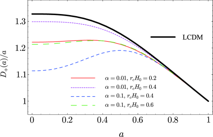
Figure 2: The growth function divided by the scale factor for different parameters. Plots are for the normal branch and $\Omega_{{\rm m}0}=0.26$.

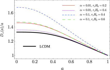
Figure 3: The growth function divided by the scale factor for different parameters. Plots are for the self-accelerating branch and $\Omega_{{\rm m}0}=0.26$.

Following Schaefer & Koyama (2008), we study a spherical overdensity with matter density $\rho_{\rm c}=\rho_{\rm c}(t)$ and radius $R=R(t)$ in a background governed by the modified Friedmann equation (2), which can be recast in

$$H^{2}=H_{0}^{2}g(\xi),\quad\xi:=\frac{8\pi G\rho}{3H_{0}^{2}}.$$ (7)

Differentiation with respect to $t$ leads to

$$\frac{\ddot{a}}{a}=H_{0}^{2}\left[g(\xi)-\frac{3}{2}\xi g^{\prime}(\xi)\right],$$ (8)

where $\dot{a}:={\rm d}a/{\rm d}t$ and $g^{\prime}:={\rm d}g/{\rm d}\xi$.

Our central assumption is that the modified gravity theory respects Birkhoff’s theorem. The dynamics of $R(t)$ is then described by

$$\frac{\ddot{R}}{R}=H_{0}^{2}\left[g(\xi_{\rm c})-\frac{3}{2}\xi_{\rm c}g^{\prime}(\xi_{\rm c})\right],$$ (9)

with

$$\xi_{\rm c}:=\frac{8\pi G\rho_{\rm c}}{3H_{0}^{2}},\quad\rho_{\rm c}\propto r^{-3}.$$ (10)

We define the overdensity as

$$\delta:=\frac{\rho_{\rm c}-\rho}{\rho}.$$ (11)

Upon linearisation the evolution equation for $\delta$ is given by

$$\ddot{\delta}+2H\dot{\delta}=4\pi G\left[g^{\prime}(\xi)+3\xi g^{\prime\prime}(\xi)\right]\rho\delta.$$ (12)

The growth function $D_{+}(a)$ is defined by $\delta(a,\mathbf{x})=D_{+}(a)\delta(a_{0},\mathbf{x})$. It follows from Eq. (12) that

$$\frac{{\rm d}^{2}}{{\rm d}a^{2}}D_{+}+\frac{f_{1}}{a}\frac{{\rm d}}{{\rm d}a}D_{+}=\frac{f_{2}}{a^{2}}D_{+},$$ (13)

where

$$f_{1} = 3+\frac{{\rm d}\ln H}{{\rm d}\ln a},$$ (14)

$$f_{2} = 3\frac{{\rm d}\ln H}{{\rm d}\ln a}+\left(\frac{{\rm d}\ln H}{{\rm d}\ln a}\right)^{2}+\frac{a^{2}}{H}\frac{{\rm d}^{2}H}{{\rm d}a^{2}}.$$ (15)

The boundary condition is given by $D_{+}(0)=0$ and $D_{+}(a_{0})=1$. Note that in standard cold dark matter dominated cosmology we find $D_{+}(a)=a$.

Figures 2 and 3 show typical behaviour of the growth function. For example, the difference between background expansion history $E(a)$ in modified gravity with $(\alpha,r_{c}H_{0})=(0.01,\,0.2)$ and that in the $\Lambda$CDM model is $\lesssim 3\,\%$, for which the growth functions differ by almost $10\,\%$ (both in the self-accelerating and normal branches). In the case of the self-accelerating branch, the growth of perturbations is suppressed compared to the $\Lambda$CDM model, in agreement with the result of Schaefer & Koyama (2008). This is because the effective dark energy term becomes dominant earlier in modified gravity than in the $\Lambda$CDM model due to the $+H^{2\alpha}$ term. In the normal branch, the effect of modified gravity works oppositely and the growth of perturbations is enhanced compared to the $\Lambda$CDM model. In the both cases, deviation from the $\Lambda$CDM result is larger for larger $\alpha$ and smaller $r_{c}$, as expected. Note here that the PPF approach predicts qualitatively the same result: structure is more evolved in the normal branch than in $\Lambda$CDM cosmology (Afshordi et al., 2008). Note also that qualitatively the same result, i.e., the suppressed (enhanced) growth function, is also found in the self-accelerating (normal) branch of the original DGP model ($\alpha=1/2$) by solving the five-dimensional Einstein equations (Cardoso et al., 2008; Song, 2008).

3.2 Spherical collapse

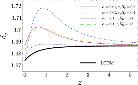
Figure 4: Overdensity at collapse time for different parameters. Plots are for the normal branch and $\Omega_{{\rm m}0}=0.26$.

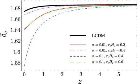
Figure 5: Overdensity at collapse time for different parameters. Plots are for the self-accelerating branch and $\Omega_{{\rm m}0}=0.26$.

In order to study spherical collapse, it is convenient to use the quantities normalised by their values at turn-around time (Wang & Steinhardt, 1998; Mota & van de Bruck, 2004; Bartelmann et al., 2006). First, we define the normalised scale factor and radius of the overdensity as follows:

$$x:=a/a_{\rm ta},\quad y:=R/R_{\rm ta}.$$ (16)

We also define the dimensionless time $\tau:=H_{\rm ta}t$, where $H_{\rm ta}:=H(a_{\rm ta})$ is the Hubble rate at turn around. Now the modified Friedmann equation can be written as

$$\frac{H^{2}}{H_{\rm ta}^{2}}=\left(\frac{\dot{x}}{x}\right)^{2}=\chi+1-\omega$$

$$\qquad\qquad\pm(H_{\rm ta}r_{c})^{-2(1-\alpha)}\left[\left(\frac{\dot{x}}{x}\right)^{2\alpha}-1\right],$$ (17)

where $\omega:=\Omega_{{\rm m}0}H_{0}^{2}/a_{\rm ta}^{3}H_{\rm ta}^{2}$, $\chi:=\omega/x^{3}$, and a dot here and hereafter denotes derivative with respect to $\tau$. This equation can be rewritten as $(\dot{x}/x)^{2}=h(\chi)$, or, equivalently,

$$\dot{x}=\sqrt{x^{2}h\left(\frac{\omega}{x^{3}}\right)}.$$ (18)

Similarly to the previous calculation, one obtains the another Friedmann equation that describes the evolution of the overdensity patch:

$$\ddot{y}=y\left[h\left(\frac{\zeta\omega}{y^{3}}\right)-\frac{3}{2}\frac{\zeta\omega}{y^{3}}h^{\prime}\left(\frac{\zeta\omega}{y^{3}}\right)\right],$$ (19)

where $h^{\prime}:={\rm d}h/{\rm d}\chi$ and $\zeta:=(\rho_{\rm c}/\rho)|_{x=1}$. The boundary condition $y|_{x=0}=0$, $\dot{y}|_{x=1}=0$, and $y|_{x=1}=1$ uniquely determines $\zeta$. Equation (19) reduces to a first order differential equation by noticing that

$$\frac{{\rm d}}{{\rm d}\tau}\dot{y}^{2}=\frac{{\rm d}}{{\rm d}\tau}\left[y^{2}h\left(\frac{\zeta\omega}{y^{3}}\right)\right].$$

From this we obtain

$$\dot{y}^{2}=y^{2}h\left(\frac{\zeta\omega}{y^{3}}\right)-h(\zeta\omega),$$ (20)

where we fixed the integration constant by using the boundary condition $\dot{y}=0$ at turn-around time ($y=1$).

Since the background dynamics at early times is the same as that of the standard matter dominant universe, we may approximate $h(\omega/x^{3})\simeq\omega/x^{3}$ for $x\ll 1$. Thus, at early times we simply have

$$\tau\simeq\frac{2}{3}\frac{x^{3/2}}{\sqrt{\omega}}.$$ (21)

Similarly, Eq. (20) reduces to

$${\rm d}\tau\simeq\sqrt{\frac{y}{\zeta\omega}}\left[1+\frac{h(\zeta\omega)}{\zeta\omega}\frac{y}{2}\right]{\rm d}y\quad\text{for}\quad y\ll 1,$$ (22)

leading to

$$\tau\simeq\frac{2}{3}\frac{y^{3/2}}{\sqrt{\zeta\omega}}\left[1+\frac{3}{10}\frac{h(\zeta\omega)}{\zeta\omega}y\right].$$ (23)

The time evolution of the nonlinear overdensity, $\Delta:=\zeta x^{3}/y^{3}$, can be computed at early times by using

$$\Delta\simeq 1+\frac{3}{5}\frac{h(\zeta\omega)}{\zeta\omega}y.$$ (24)

The linear density contrast at collapse time, $\delta_{c}$, can be used to relate the nonlinear overdensity $\Delta$ with the density that would result from linear evolution and the same initial condition. Using the growth function, we have

$$\delta_{\rm c}:=\lim_{x\to 0}\frac{D_{+}(x_{\rm c})}{D_{+}(x)}\left[\Delta(x)-1\right].$$ (25)

We numerically computed $\delta_{c}(z)$ for various model parameters, and the results are illustrated in Figs. 4 and 5. We find that modified gravity does not change $\delta_{c}$ much: for example, $\delta_{c}$ in modified gravity with $(\alpha,r_{c}H_{0})=(0.01,\,0.2)$ differs from the $\Lambda$CDM prediction by 1 – $2\,\%$ (both in the self-accelerating and normal branches).

4 The Sunyaev-Zel’dovich power spectrum

In this section, we investigate the effect of modified gravity on the SZ angular power spectrum. Modification of gravity changes cluster number count through the modified growth function and critical density contrast. We concentrate on the case of the normal branch. The SZ angular power spectrum could be amplified in this branch because the growth function is enhanced relative to the $\Lambda$CDM model. The change in the critical density contrast is quite small, and hence it will give rise to only a negligible effect.

Modified gravity might in general affect the halo profiles assumed in the following discussion. This issue can be addressed by evaluating the Vainshtein radius, $r_{*}$, below which Einstein gravity is recovered. The Vainshtein radius in this particular model is given by $r_{*}=[r_{c}^{4(1-\alpha)}r_{{\rm S}}]^{1/[1+4(1-\alpha)]}\simeq[r_{c}^{4}r_{{\rm S}}]^{1/5}$, where $r_{{\rm S}}$ is the Schwarzschild radius of the source (Dvali, 2006). More explicitly, one has $r_{*}\sim 10^{2}[(r_{c}H_{0})^{4}(M/M_{\odot})]^{1/5}\,$kpc, and for $r_{c}H_{0}\sim 0.01$ and $M\sim 10^{14}\,M_{\odot}$, $r_{*}\sim 1\,$Mpc. This estimate allows us to employ the halo profiles used in the context of standard gravity.

The computation of the SZ angular power spectrum is based on the halo formalism (Cole & Kaiser, 1988; Makino & Suto, 1993; Komatsu & Kitayama, 1999; Komatsu & Seljak, 2002). Since the one-halo Poisson term dominates the halo-halo correlation term on the scales we are interested in, we neglect the halo-halo correlation term. The SZ angular power spectrum is then given by

$$C_{\ell}^{SZ}=g_{\nu}^{2}\int_{0}^{z_{\rm max}}\!{\rm d}z\frac{{\rm d}V}{{\rm d}z}\int_{M_{\rm min}}^{M_{\rm max}}\!{\rm d}M\frac{{\rm d}n(M,z)}{{\rm d}M}\left|y_{\ell}(M,z)\right|^{2},$$ (26)

where $V(z)$ is the comoving volume at $z$ per steradian, ${\rm d}n(M,z)/{\rm d}M$ is the number density of clusters, $\tilde{y}_{l}(M,z)$ is the 2D Fourier transform of the projected Compton $y$-parameter, and $g_{\nu}$ is the spectral function of the SZ effect, which is given by

$$g_{\nu}={x^{2}e^{x}\over(e^{2x}-1)^{2}}\left[x\coth\left({1\over 2}x\right)-4\right],$$ (27)

where $x=h\nu/k_{B}T_{\gamma}$ with the Boltzmann constant $k_{B}$ and the CMB temperature $T_{\gamma}$.

As we are considering the spherical collapse scenario for the formation of halos, we utilise the Press-Schechter theory (Press & Schechter, 1974),

$${{\rm d}n(M,z)\over{\rm d}M}=\sqrt{2\over\pi}{\rho\over M}\left[-{\delta_{c}\over\sigma(M,z)}{\partial\sigma\over\partial M}\right]\exp\left[-{\delta_{c}^{2}\over 2\sigma(M,z)}\right],$$ (28)

where $\delta_{c}$ is the critical over density which is obtained in the previous section, $\sigma(M,z)$ is the variance of the matter density field on the mass scale $M$. The variance $\sigma$ is computed from the power spectrum of linear matter density fluctuations with the top hat filter,

$$\sigma^{2}(M,z)=\int{\rm d}k\,k^{2}P_{\rm m}(k,z)W(kR),$$ (29)

where $W(kR)$ is the top hat window function and $R$ is the scale which corresponds to $M(=4\pi\rho R^{3}/3)$. We calculate the linear power spectrum $P_{\rm m}(k,z)$ in the modified gravity model by using the growth function obtained in the previous section and the initial condition for the curvature perturbation and the scalar spectral index, $\Delta^{2}_{\cal R}=2.41\times 10^{-9}$, $n=0.96$, given by WMAP (Komatsu et al., 2009).

The 2D Fourier transform of the projected Compton $y$-parameter is given by

$$y_{\ell}={4\pi r_{\rm s}\over\ell_{\rm s}^{2}}\int_{0}^{\infty}{\rm d}x\,x^{2}y_{3d}(x){\sin(\ell x/\ell_{\rm s})\over\ell x/\ell_{\rm s}},$$ (30)

where $y_{3d}$ is the radial profile of the Compton $y$-parameter,

$$y_{3d}(x)={\sigma_{\rm T}\over m_{e}}~{}n_{e}(x)k_{\rm B}T_{e}(x),$$ (31)

with $\sigma_{\rm T}$ being the Thomson cross section and $m_{e}$ the electron mass. $\ell_{\rm s}$ is the angular wavenumber corresponding to $r_{\rm s}$, $\ell_{\rm s}=D_{A}/r_{\rm s}$, with $D_{A}$ being the angular diameter distance.

For the electron density profile $n_{e}$ and the temperature profile $T_{e}$, we use the result of Komatsu & Seljak (2002), which is based on the NFW dark matter density profile (Navarro et al., 1997). The NFW dark matter density profile is given by

$$\rho_{\rm DM}(x)=\frac{\rho_{\rm s}}{x(1+x)^{2}},$$ (32)

where $x:=r/r_{\rm s}$ where $r_{\rm s}$ is a scale radius, and $\rho_{\rm s}$ is a scale density. The scale radius $r_{\rm s}$ is related to the virial radius by the concentration parameter $c$ as

$${r_{\rm s}(M,z)}={r_{\rm vir}(M,z)\over c(M,z)}.$$ (33)

We use the concentration parameter of Komatsu & Seljak (2002),

$$c(M,z)\approx\frac{10}{1+z}\left[\frac{M}{M_{*}(0)}\right]^{-0.2},$$ (34)

where $M_{*}(0)$ is a solution to $\sigma(M,0)=\delta_{c}$ at the redshift $z=0$.

We adopt the spherical collapsed model to obtain the virial radius,

$$r_{\rm vir}(M,z)={3M\over 4\pi\Delta_{v}(z)\rho(z)},$$ (35)

where $\Delta_{v}(z)$ is the virialised overdensity at $z$. Modified gravity changes the virialised overdensity, which we compute following Schmidt et al. (2009). For example, the modified virial overdensity at $z=0$ is $\Delta_{v}=270$ for $(\alpha,r_{c}H_{0})=(0.1,0.3)$ and $\Delta_{v}=300$ for $(\alpha,r_{c}H_{0})=(0.1,0.4)$, while $\Delta_{v}=370$ in the $\Lambda$CDM model. Thus, we find that the actual density in a virialised halo, $\Delta_{v}(z)\rho(z)$, is lower in modified gravity than in the $\Lambda$CDM model.

In order to obtain the profiles of the electron density and temperature, Komatsu & Seljak (2002) assumed three things: (i) the electron gas is in hydrostatic equilibrium in the dark matter potential; (ii) the electron gas density follows the dark matter density in the outer part of the halo; (iii) the equation of state of the electron gas is polytropic, $P_{e}\propto\rho_{e}^{\gamma}$, where $P_{e}$, $\rho_{e}$ and ${\gamma}$ are the electron gas pressure, the gas density and the polytropic index, respectively. Under these assumptions, the electron number density and temperature profiles are simply given by

$$n_{e} = n_{e\rm c}F(x),$$ (36)

$$T_{e} = T_{e\rm c}F^{\gamma-1}(x).$$ (37)

Here, $n_{e\rm c}$ and $T_{e\rm c}$ are the electron density and temperature at the centre, respectively, and the dimensionless profile $F(x)$ is written as

$$F(x)=\left\{1-A\left[1-{\ln(1+c)\over x}\right]\right\}^{1/(\gamma-1)},$$ (38)

where the coefficient $A$ is defined as

$$A:=3\eta^{-1}_{\rm c}\frac{\gamma-1}{\gamma}\left[\frac{\ln(1+c)}{c}-\frac{1}{1+c}\right]^{-1}.$$ (39)

The central electron density $n_{e\rm c}$ and the temperature $T_{e\rm c}$ are given by

$$n_{e\rm c} = 3.01\left({M\over 10^{14}M_{\odot}}\right)\left({r_{\rm vir}\over 1~{}{\rm Mpc}}\right)^{-3}$$ (40)

$$\!\!\!\!\!\!\!\!\!\times\frac{c}{(1+c)^{2}}\left[\ln(1+c)-\frac{c}{1+c}\right]^{-1}F^{-1}(c)~{}{\rm cm}^{-3},$$

$$T_{e\rm c} = 0.88~{}\eta_{\rm c}\left[M/(10^{14}h^{-1}M_{\odot})\over r_{\rm vir}/(1h^{-1}{\rm Mpc})\right]~{}{\rm keV}.$$ (41)

For $\gamma$ and $\eta_{\rm c}$, Komatsu & Seljak (2002) provided the following useful fitting formulas:

$$\gamma=1.137+8.94\times 10^{-2}\ln(c/5)-3.68\times 10^{-3}(c-5),$$ (42)

$$\eta_{\rm c}=2.235+0.202(c-5)-1.16\times 10^{-3}\left(c-5\right)^{2}.$$ (43)

Figure 6 shows the SZ power spectrum in the modified gravity model. We take three sets of the model parameters: $(\alpha,r_{c}H_{0})=(0.1,0.2)$ , $(0.1,0.3)$, and $(0.1,0.4)$, giving $\sigma_{8}=1.2$, $1.0$ and $0.9$, respectively (The initial density power spectra are the same for all of these parameter sets). For comparison, we plot in Fig. 6 the SZ power spectra in the $\Lambda$CDM models with $\sigma_{8}=0.77$ (our fiducial model) and with $\sigma_{8}=1.0$. One sees that the amplitude of the peak in modified gravity is lower than that in the $\Lambda$CDM model with the same $\sigma_{8}$. This is because the actual density in a virialised halo is lower in modified gravity than in the $\Lambda$CDM model.

Moreover, modified gravity shows the damping of the SZ power spectrum on small scales and the amplification on large scales, because the contribution from halos at high redshifts in modified gravity is smaller than that in the $\Lambda$CDM model. The redshift contribution for different $\ell$ is shown in Fig. 7. The growth of matter density fluctuations in the modified gravity model is rapid at late times compared with the growth in the $\Lambda$CDM model with the same $\sigma_{8}$. As a result, the formation of halos delays, leading to the large contribution from low redshifts and small contribution from high redshifts.

The SZ power spectrum is constrained by the CMB observations on small scales. In the $\Lambda$CDM model the ACBAR data at $\ell\sim 2500$ gives the constraint on the SZ power spectrum in terms of $\sigma_{8}$: $\sigma_{8}<1$ (Kuo et al., 2007). The peak amplitude of the SZ power spectrum is lower in modified gravity than in the $\Lambda$CDM model with the same $\sigma_{8}$. This result then yields the constraint from the ACBAR data $\sigma_{8}<1.2$ in modified gravity. Figure 8 shows $\sigma_{8}$ as a function of the model parameters $\alpha$ and $r_{c}H_{0}$. In the limit $r_{c}\to\infty$, $\sigma_{8}$ reduces to the value in our fiducial model, $\sigma_{8}=0.77$. From the ACBAR experiment, the parameter region below the $\sigma_{8}=1.2$ line in Fig. 8 is excluded.

Stronger constraints can be obtained from the small angular scale CMB measurements by the QUaD experiment (Friedman et al., 2009). The QUaD telescope measured the CMB temperature anisotropy in the multipole range $2000<\ell<3000$ at 150 GHz. The QUaD team reported no strong evidence of the SZ effect and the result is consistent with the WMAP data which yields $\sigma_{8}\sim 0.8$. Therefore, using the result of the QUaD experiment to constrain $\sigma_{8}$, the modified gravity parameters are more strongly restricted than in the case of the ACBAR data. The constraint from the QUaD data gives $\sigma_{8}\sim 0.9$ in modified gravity.

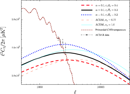
Figure 6: SZ angular power spectra for different modified gravity parameters. The dotted, solid, and dashed lines represent SZ power spectra for $(\alpha,r_{c}H_{0})=(0.1,0.2)$, $(0.1,0.3)$, and $(0.1,0.4)$, respectively. The SZ angular power spectra for $\sigma_{8}=1.0$ and $\sigma_{8}=0.77$ in the $\Lambda$CDM model are shown as the thin solid and thin dashed lines, respectively. For references, we plot the primordial CMB temperature angular power spectrum in our fiducial $\Lambda$CDM model and the ACBAR data.

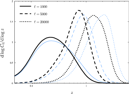
Figure 7: Distribution of the redshift contribution of the SZ angular power spectrum for different $\ell$ modes. We set the modified gravity parameters $\alpha=0.1$ and $r_{c}H_{0}=0.3$. The solid, the dashed, and the dotted lines represent the distributions for $\ell=1000$, $\ell=5000$, and $\ell=20000$, respectively. For comparison, we plot the distributions for the $\Lambda$CDM model with $\sigma_{8}=1.0$ as thin lines.

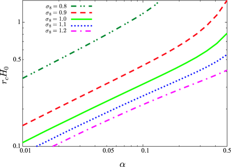
Figure 8: The amplitude $\sigma_{8}$ as a function of modified gravity parameter $\alpha$ and $r_{c}$. The dashed-dotted-dotted, dashed, solid, dotted, dashed-dotted lines represent $\sigma_{8}=0.8$, $0.9$, $1.0$, $1.1$ and $1.2$.

5 Conclusions

In this paper, we have explored observational consequences of structure formation in modified gravity. The model considered is a phenomenological extension of the DGP braneworld, and modification to the standard $\Lambda$CDM model is characterized by the additional term $\pm H^{2\alpha}/r_{c}^{2(1-\alpha)}$ in the Friedmann equation. In the case of $\alpha=1/2$, the term arises from the five-dimensional effect, but in this work $\alpha$ and $r_{c}$ were assumed to be free parameters.

First, we have studied the spherical collapse model of nonlinear structure formation in modified gravity. It was found that change in the growth function is relatively large, but the linear density contrast for spherical collapse undergoes very small modification. For the self-accelerating branch, the growth of perturbations is suppressed compared to the $\Lambda$CDM model, which confirms qualitatively the result of Schaefer & Koyama (2008). For the normal branch, the growth of perturbations is enhanced compared to the $\Lambda$CDM model.

Focusing on the normal branch, we then investigated the effect of modified gravity on the SZ angular power spectrum. The enhanced growth function in the normal branch results in the amplification of $\sigma_{8}$. However, the modification to the SZ power spectrum is rather nontrivial. The peak amplitude of the SZ angular power spectrum is lower in modified gravity than in the $\Lambda$CDM model with the same $\sigma_{8}$, because halos are virialised at lower density in modified gravity than in the $\Lambda$CDM model. In addition to this, modified gravity shows the damping of the SZ power spectrum on small scales.

We confronted the modified SZ spectrum with CMB observations on small scales. Observational constraints can be read off from Fig. 8. The ACBAR experiment gives the constraint on the SZ power spectrum which translates to $\sigma_{8}=1.2$ in modified gravity. From this we put constraints to the parameters of the modified gravity model: for example, we have $r_{c}H_{0}>0.4$ for $\alpha=0.5$ and $r_{c}H_{0}>0.2$ for $\alpha=0.1$. The QUaD data gives severer constraints on the parameters: $\sigma_{8}=0.9$, leading to $r_{c}H_{0}>0.4$ for $\alpha=0.1$.

Appendix A Comparison with different approaches

In the phenomenologically extended version of the DGP model, different assumptions can be made in computing the growth of perturbations. Instead of using Birkhoff’s theorem, we may assume that the behaviour of perturbations is governed by a scalar-tensor theory. Following Koyama (2006), we now compare the linear evolution of perturbations obtained by these two approaches. If one does not assume Birkhoff’s theorem but employs a scalar-tensor theory as an effective theory for perturbations, the evolution of $\delta$ will be described by (Koyama, 2006)

$$\ddot{\delta}+2H\dot{\delta}=4\pi G\left(1+\frac{1}{3\beta}\right)\rho\delta,$$ (44)

where

$$\beta:=1+\frac{(r_{c}H)^{2(1-\alpha)}}{\alpha}\left[1+\frac{2}{3}\frac{(1-\alpha)\dot{H}}{H^{2}}\right].$$ (45)

Note that this is the expression for the normal branch. We denote by $D_{+}^{\star}(a)$ the growth function calculated from this equation. The difference between $D_{+}^{\star}$ and $D_{+}$ obtained in the main text, $(D_{+}^{\star}-D_{+})/(D_{+}^{\star}+D_{+})$, is presented in Fig. 9. As can be seen, there is only a few percent difference between the two approaches concerning the linear growth of perturbations. Developing nonlinear theory with the violation of Birkhoff’s theorem taken into account is beyond the scope of the present paper.

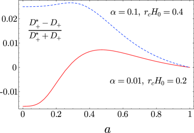
Figure 9: Comparison with the growth functions obtained by the different approaches.

References

- Afshordi et al. (2008) Afshordi N., Geshnizjani G., Khoury J., 2008, arXiv, 0812.2244
- Bartelmann et al. (2006) Bartelmann M., Doran M., Wetterich C., 2006, Astron. Astrophys., 454, 27
- Bekenstein (2004) Bekenstein J. D., 2004, Phys. Rev., D70, 083509
- Cardoso et al. (2008) Cardoso A., Koyama K., Seahra S. S., Silva F. P., 2008, Phys. Rev., D77, 083512
- Cole & Kaiser (1988) Cole S., Kaiser N., 1988, Mon. Not. Roy. Astron. Soc., 233, 637
- de Rham et al. (2008a) de Rham C., et al., 2008a, JCAP, 0802, 011
- de Rham et al. (2008b) de Rham C., et al., 2008b, Phys. Rev. Lett., 100, 251603
- Deffayet et al. (2002) Deffayet C., Dvali G. R., Gabadadze G., 2002, Phys. Rev., D65, 044023
- Dvali (2006) Dvali G., 2006, New J. Phys., 8, 326
- Dvali & Turner (2003) Dvali G., Turner M. S., 2003, arXiv, astro-ph/0301510
- Dvali et al. (2000) Dvali G. R., Gabadadze G., Porrati M., 2000, Phys. Lett., B485, 208
- Friedman et al. (2009) Friedman R. B., et al., 2009, arXiv, 0901.4334
- Hu & Sawicki (2007) Hu W., Sawicki I., 2007, Phys. Rev., D76, 104043
- Kaloper & Kiley (2007) Kaloper N., Kiley D., 2007, JHEP, 05, 045
- Khoury & Wyman (2009) Khoury J., Wyman M., 2009, arXiv, 0903.1292
- Kobayashi (2008) Kobayashi T., 2008, Phys. Rev., D78, 084018
- Komatsu et al. (2009) Komatsu E., et al., 2009, Astropys.J. S., 180, 330
- Komatsu & Kitayama (1999) Komatsu E., Kitayama T., 1999, Astrophys. J., 526, L1
- Komatsu & Seljak (2002) Komatsu E., Seljak U., 2002, Mon. Not. Roy. Astron. Soc., 336, 1256
- Koyama (2006) Koyama K., 2006, JCAP, 0603, 017
- Koyama & Silva (2007) Koyama K., Silva F. P., 2007, Phys. Rev., D75, 084040
- Kuo et al. (2007) Kuo C. L., et al., 2007, Astrophys. J., 664, 687
- Lue et al. (2004) Lue A., Scoccimarro R., Starkman G. D., 2004, Phys. Rev., D69, 124015
- Lue & Starkman (2003) Lue A., Starkman G., 2003, Phys. Rev., D67, 064002
- Makino & Suto (1993) Makino N., Suto Y., 1993, Astrophys. J., 405, 1
- Martino et al. (2008) Martino M. C., Stabenau H. F., Sheth R. K., 2008, arXiv, 0812.0200
- Milgrom (1983) Milgrom M., 1983, Astrophys. J., 270, 384
- Mota & van de Bruck (2004) Mota D. F., van de Bruck C., 2004, Astron. Astrophys., 421, 71
- Navarro et al. (1997) Navarro J. F., Frenk C. S., White S. D. M., 1997, ApJ, 490, 493
- Press & Schechter (1974) Press W. H., Schechter P., 1974, Astrophys. J., 187, 425
- Schaefer & Koyama (2008) Schäfer B. M., Koyama K., 2008, Mon. Not. Roy. Astron. Soc., 385, 411
- Schmidt (2008) Schmidt F., 2008, Phys. Rev., D78, 043002
- Schmidt et al. (2009) Schmidt, F. and Lima, M. and Oyaizu, H. and Hu, W., 2009, Phys. Rev., D79, 083518
- Sealfon et al. (2005) Sealfon C., Verde L., Jimenez R., 2005, Phys. Rev., D71, 083004
- Shirata et al. (2005) Shirata A., Shiromizu T., Yoshida N., Suto Y., 2005, Phys. Rev., D71, 064030
- Shirata et al. (2007) Shirata A., Suto Y., Hikage C., Shiromizu T., Yoshida N., 2007, Phys. Rev., D76, 044026
- Song (2008) Song Y.-S., 2008, Phys. Rev., D77, 124031
- Sotiriou & Faraoni (2008) Sotiriou T. P., Faraoni V., 2008, arXiv, 0805.1726
- Stabenau & Jain (2006) Stabenau H. F., Jain B., 2006, Phys. Rev., D74, 084007
- Tanaka (2004) Tanaka T., 2004, Phys. Rev., D69, 024001
- Thomas et al. (2008) Thomas S. A., Abdalla F. B., Weller J., 2008, arXiv, 0810.4863
- Wang & Steinhardt (1998) Wang L.-M., Steinhardt P. J., 1998, Astrophys. J., 508, 483