Dynamics of Strings between Domain Walls

Abstract

Configurations of vortex-strings stretched between or ending on domain walls were previously found to be 1/4 BPS states. Among zero modes of string positions, the center of mass of strings in each region between two adjacent domain walls is shown to be non-normalizable whereas the rests are normalizable. We study dynamics of vortex-strings stretched between separated domain walls by using two methods, the moduli space (geodesic) approximation of full 1/4 BPS states and the charged particle approximation for string endpoints in the wall effective action. In the first method we obtain the effective Lagrangian explicitly and find the 90 degree scattering for head-on collision. In the second method the domain wall effective action is assumed to be $U(1)^{N}$ gauge theory, and we find a good agreement between two methods for well separated strings. This paper is based on our work 1 .

1 Composite solitons of walls and vortices

Our model is $d=3+1$ $U(1)$ gauge theory with $N_{\rm F}(\geq 2)$ fundamental Higgs fields and an adjoint scalar field.

$$\mathcal{L} =-\frac{1}{2g^{2}}F_{\mu\nu}F^{\mu\nu}+\frac{1}{g^{2}}\partial_{\mu}\Sigma\partial^{\mu}\Sigma+\mathcal{D}_{\mu}H(\mathcal{D}^{\mu}H)^{\dagger}$$

$$-\frac{g^{2}}{4}\left(HH^{\dagger}-c\right)^{2}+(HM-\Sigma H)(HM-\Sigma H)^{\dagger}.$$ (1)

The model can embedded into a ${\cal N}=2$ supersymmetric gauge theory with non-zero FI parameters. Vacua of this model are characterized by one flavor index $\langle A\rangle$

$$H^{A}=\sqrt{c},\quad H^{B}=0\,\,(B\neq A),\quad\Sigma=m_{A}.$$ (2)

There are $N_{\rm F}$ discrete vacua labeled by $\langle A\rangle$, and there exist 1/2 BPS domain walls dividing them walls . Furthermore, vortices can live in each vacuum breaking further 1/2 supersymmetries. The 1/4 BPS equations can be obtained aswalls and vortices

$${\cal D}_{1}\Sigma-F_{23}=0,\quad{\cal D}_{2}\Sigma-F_{31}=0,$$ (3)

$${\cal D}_{3}\Sigma-F_{12}-\frac{g^{2}}{2}\left(c{\bf 1}_{N_{\rm C}}-HH^{\dagger}\right)=0,$$ (4)

$${\cal D}_{1}H+i{\cal D}_{2}H=0,\quad{\cal D}_{3}H+\Sigma H-HM=0.$$ (5)

Configurations of vortices and domain walls are illustrated in Fig.1.

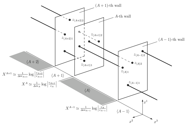
Figure 1: Composite solitons of walls and vortices

2 Dynamics of vortices between domain walls

Dynamics of solitons can be investigated by moduli space approximation Manton . We give the weak time dependence to normalizable moduli parameters, and look at the time evolution of them. Geodesic motions on the moduli space correspond to actual motion of solitons. Here let us focus on $N_{\rm F}=3$ with masses $M=(m,0,-m)$ and consider the configuration with two domain walls and two vortices in the middle vacuum. Such exact solution can be obtained in strong coupling limit $g\to\infty$.

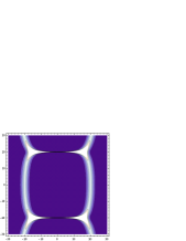
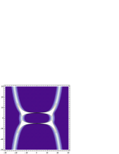
$z_{0}=20$	$z_{0}=5$	$z_{0}=0$

Figure 2: The energy densities in a plane containing vortices. Vertical lines are walls and horizontal lines are vortices.

Normalizable moduli parameter in the solution is only relative distance between two vortices $z_{0}$. Distance between domain walls is controlled by non-normalizable moduli parameter $v$. The energy densities in a plane containing vortices with various $z_{0}$ and $v=e^{4}$ are shown in Fig.2.

Let us now give the weak time dependence to $z_{0}$, and investigate the dynamics of the middle vortices. We can obtain the Kähler metric as an integral over the complete elliptic integral of the second kind $E(k)$

$$K_{z_{0}\bar{z}_{0}} =2\pi c\int dx_{3}\,kE(k),$$

$$\quad{\rm with}\quad k=\left(\frac{|vz_{0}^{2}|^{2}}{2\cosh mx_{3}+|vz_{0}^{2}|^{2}}\right)^{1/2}.$$ (6)

If we expand the Kähler metric around $|vz_{0}^{2}|^{2}=0$, we obtain

$$dx^{2} =2K_{z_{0}\bar{z}_{0}}dz_{0}d\bar{z}_{0}$$

$$=\frac{\pi^{\frac{3}{2}}|v|c}{4m}\Bigl{(}\Gamma(1/4)^{2}-\frac{3}{2}\Gamma(3/4)^{2}|vZ|^{2}$$

$$\qquad\qquad\qquad\qquad+\mathcal{O}(|vZ|^{4})\Bigr{)}dZd\bar{Z}.$$ (7)

Since the coordinate $Z\equiv z_{0}^{2}$ is a good coordinate even at the origin, it shows that the moduli space is non-singular at the origin and the vortices scatter with right-angle in head-on collisions. If we take the opposite limit $|vz_{0}^{2}|^{2}\to\infty$, the metric can be calculated as

$$K_{z_{0}\bar{z}_{0}}\approx\frac{8\pi c}{m}\log|4vz_{0}^{2}|.$$ (8)

Since the domain walls are logarithmically bending in the present case, the definition of the distance between domain walls is not clear. However, at the center of mass of two vortices, the distance between domain walls is given by

$$l_{\langle 2\rangle}=\frac{4}{m}\log|vz_{0}^{2}|.$$ (9)

It can be considered as the typical lengths of the vortices (see Fig.2). Therefore, the above asymptotic metric (8) can be understood as the kinetic energy of two vortices.

3 Vortices as charged particles

So far, we have calculated the metric on the 1/4 BPS moduli space and investigated the dynamics of vortices suspended between the domain walls, using the moduli space approximation. Now let us obtain the vortex dynamics from effective theory on domain walls. Effective theory on $N$ domain walls is given by $N$ scalar fields $\Phi_{A}$ and $N$ compact scalar fields $\sigma_{A}$, which correspond to positions and phases of domain walls, respectively. If we take the dual of compact scalar fields in $d=2+1$, we obtain $U(1)^{N}$ gauge theory as the effective theory on domain walls

$${\cal L}_{\rm w}=\sum_{A=1}^{N}\left[\frac{1}{2e^{2}_{A}}\partial_{\mu}\Phi^{A}\partial^{\mu}\Phi^{A}-\frac{1}{4e^{2}_{A}}F_{\mu\nu}^{A}F^{A\,\mu\nu}\right].$$ (10)

Here we assume $N$ domain walls are all well-separated. Vortices can be viewed as charged particles in the effective theory, which are sources of scalar fields and electric fields on the neighboring domain walls. Let us consider the $i$-th vortex living in vacuum $\langle B\rangle$ positioned at $z_{\left<B\right>i}$ with a velocity $\dot{z}_{\left<B\right>i}=u_{\left<B\right>i}$. It yields the scalar field and the electric field on the worldvolume of neighboring domain walls

$$(\Phi^{A})_{(B,i)} =\phantom{-}(\delta_{A+1,B}-\delta_{AB})\frac{e^{2}_{A}}{2\pi}G(u_{\left<B\right>i};z-z_{\left<B\right>i}),$$ (11)

$$(A_{\mu}^{A})_{(B,i)} =-(\delta_{A+1,B}-\delta_{AB})\frac{e^{2}_{A}}{2\pi}\frac{v_{\mu\left<B\right>i}}{\sqrt{1-|u_{\left<B\right>i}|^{2}}}$$

$$\qquad\qquad\times G(u_{\left<B\right>i};z-z_{\left<B\right>i}).$$ (12)

where $v^{\mu}_{\left<B\right>i}=(1,{\rm Re}[u_{\left<B\right>i}],{\rm Im}[u_{\left<B\right>i}])$ and $G$ is the Green’s function given by

$$G(u_{\left<B\right>i};z-z_{\left<B\right>i})=\log|L_{u_{\left<B\right>i}}(z-z_{\left<B\right>i})|-\log L+f(u_{\left<B\right>i}).$$ (13)

We can regard the dynamics of the vortex living in vacuum $\langle A\rangle$ as an electric charge moving in the background potential produced by the other vortices. The Lagrangian for the $i$-th particle in vacuum $\langle A\rangle$ is then given by

$$L_{i}^{\langle A\rangle} =\sum_{B}(\delta_{A,B}-\delta_{A-1,B})\left(-\widetilde{\Phi}^{B}\sqrt{1-|u_{\left<A\right>i}|^{2}}-\widetilde{A}_{\mu}^{B}v^{\mu}_{\left<A\right>i}\right)$$

$$\approx\sum_{B}(\delta_{A,B}-\delta_{A-1,B})\left(-\widetilde{\Phi}^{B}+\frac{\widetilde{\Phi}^{B}}{2}|u_{\left<A\right>i}|^{2}-\widetilde{A}_{\mu}^{B}v^{\mu}_{\left<A\right>i}\right),$$ (14)

where $\widetilde{\Phi}^{B},\,\widetilde{A}_{0}^{B},\,\widetilde{\mathbf{A}}^{B}$ are the values of the fields produced by the other particles at the location of the particle $z=z_{\left<A\right>i}$

$$\widetilde{\Phi}^{B} \equiv \langle\Phi^{B}\rangle+\sum_{(C,j)}(\Phi^{B})_{(C,j)}\big{|}_{z=z_{\left<A\right>i}},$$ (15)

$$\widetilde{A}_{\mu}^{B} = \sum_{(C,j)}(A_{\mu}^{B})_{(C,j)}\big{|}_{z=z_{\left<A\right>i}}.$$ (16)

Similar method is well-known for monopoles in $3+1$ dimensions monopoles .

The above procedure yields the effective Lagrangian for the relative motion of two vortices which we have investigated in the last section as

$$L_{\rm eff}=\left(\frac{8\pi c}{m}\log|vz_{0}^{2}|+\frac{16\pi c}{m}\log 2\right)|\dot{z}_{0}|^{2}.$$ (17)

This coincides with the asymptotic result in Eq.(8).

Here we have not shown other examples. However, we can show that this method correctly reproduces the asymptotic metric on the moduli space when the domain walls are well-separated in $x_{3}$-direction, and the vortices are well-separated from other vortices in $z$-plane.

References

• (1) M. Eto, T. Fujimori, T. Nagashima, M. Nitta, K. Ohashi and N. Sakai, Phys. Rev. D 79, 045015 (2009);
• (2) E. R. C. Abraham and P. K. Townsend, Phys. Lett. B 291, 85 (1992); Phys. Lett. B 295, 225 (1992). J. P. Gauntlett, D. Tong and P. K. Townsend, Phys. Rev. D 64, 025010 (2001) [arXiv:hep-th/0012178]; D. Tong, Phys. Rev.  D 66, 025013 (2002) [arXiv:hep-th/0202012]; Y. Isozumi, M. Nitta, K. Ohashi and N. Sakai, Phys. Rev. Lett.  93, 161601 (2004) [arXiv:hep-th/0404198]; Phys. Rev. D 70, 125014 (2004) [arXiv:hep-th/0405194];
• (3) M. Shifman and A. Yung, Phys. Rev.  D 67, 125007 (2003) [arXiv:hep-th/0212293]. D. Tong, Phys. Rev. D 69, 065003 (2004) [arXiv:hep-th/0307302]; Y. Isozumi, M. Nitta, K. Ohashi and N. Sakai, Phys. Rev. D 71 (2005) 065018 [arXiv:hep-th/0405129].
• (4) N. S. Manton, Phys. Lett. B 110, 54 (1982).
• (5) N. S. Manton, Phys. Lett.  B 154, 397 (1985) [Erratum-ibid.  157B, 475 (1985)]. G. W. Gibbons and N. S. Manton, Phys. Lett.  B 356, 32 (1995) [arXiv:hep-th/9506052].