Multi-terminal spin-dependent transport in ballistic carbon nanotubes

Abstract

We study theoretically non-local spin-transport in a ballistic carbon nanotube contacted to two ferromagnetic leads and two normal metal leads. When the magnetizations of the two ferromagnets are changed from a parallel to an antiparallel configuration, the circuit shows an hysteretic behavior which is specific to the few-channels regime. In the coherent limit, the amplitude of the magnetic signals is strongly enhanced due to resonance effects occuring inside the nanotube. Our calculations pave the way to new experiments on low-dimensional non-local spin-transport, which should give results remarkably different from the experiments realized so far in the multichannel diffusive incoherent regime.

I Introduction

Non-local electric effects have been observed since the early days of mesoscopic physics, e.g. in metallic circuitsWebb:89 ; FilsMetal . This fact is related to the primarily non-local nature of electronic wave functions in quantum coherent conductors. The spin-degree of freedom has raised little attention in this context, although its control and detection is one of the major challenges of nanophysics, nowadays. Non-local spin signals have been studied for multi-terminal metallic conductorsJohnson ; Jedema ; Jedema2 ; Zaffalon , semiconductorsLou and grapheneTombros2 , in the multichannel diffusive incoherent (MDI) regime. It has been found that a non-equilibrium spin accumulation induced by a ferromagnet into a given conductor can be detected as a voltage across the interface between this conductor and another ferromagnetSilsbee . However, to our knowledge, spin-dependent non local effects have not been investigated in the coherent regime, so far.

Carbon-nanotubes-based circuits are appealing candidates for observing a non-local, spin-dependent, and coherent behavior of electrons. First, electronic transport in carbon nanotubes (CNTs) can reach the few-channels ballistic regime, as suggested by the observation of Fabry-Perot-like interference patternsLiang . Secondly, spin injection has already been demonstrated in CNTs connected to two ferromagnetic leads (see Ref. SST, for a review). Thirdly, non local voltages have been observed in CNTs contacted to four normal-metal leadsMakarovski , which suggests that electrons can propagate in the nanotube sections below the contacts. The study of non-local spin transport in CNTs has recently triggered some experimental effortsTombros ; Gunnar ; Cheryl . However, a theoretical insight on this topic is lacking. Some major questions to address are what are the signatures of a non-local and spin-dependent behavior of electrons in a nanoconductor, and to which extent these signatures are specific to the coherent regime or the few-channels case.

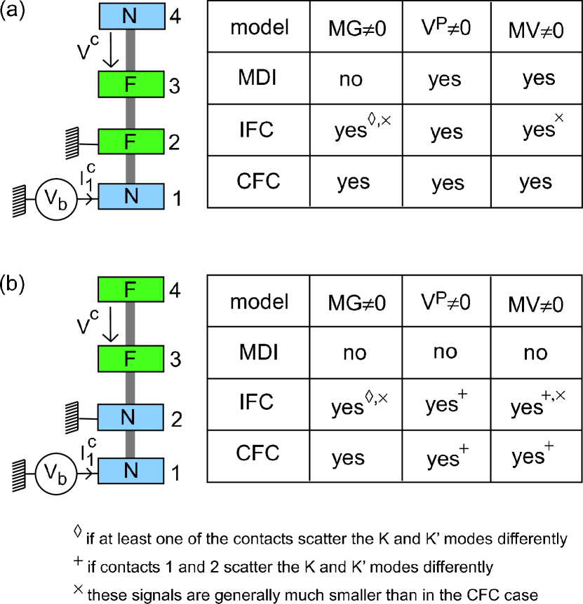
Figure 1: Left: The two types of circuits [setups (a) and (b)] studied in this article. The central conductor (represented with the grey bar) is contacted to two normal metal leads $N$ and two ferromagnetic leads $F$, which can be magnetized in parallel ($c=P$) or antiparallel ($c=AP$) configurations. The only difference between setups (a) and (b) is the position of the two $F$ leads. Contacts 1 and 2 are used as source and drain to measure a local conductance $G^{c\text{ }}$and contacts 3 and 4 are used to probe a non-local voltage $V^{c}$ outside the classical current path. Right: Tables presenting the behaviors of setups (a) and (b) in various regimes. We study the existence of the signals $MG=(G^{P}-G^{AP})/G^{P}$, $V^{P}$ and $MV=(V^{P}-V^{AP})/V_{b}$. We compare the predictions of the coherent four-channels model (CFC) of section IV, the incoherent four-channels model (IFC) of section V and the multichannel diffusive incoherent (MDI) model of section III.

In this paper, we study the behavior of a CNT with two normal metal ($N$) leads and two ferromagnetic ($F$) leads magnetized in colinear directions. Two leads are used as source and drain to define a local conductance $G^{c\text{ }}$and the other two are used to probe a non-local voltage $V^{c}$ outside the classical current path. We consider two different setups which differ on the positions of the $F$ leads. Setup (a) corresponds to the standard geometry used for the study of the MDI limit. In setup (b), the two $F$ leads play the role of the voltage probes, so that no magnetic response is allowed in the MDI limit. We mainly focus on the coherent regime, using a scattering description with two transverse modes, to account for the twofold orbital degeneracy commonly observed in CNTsdeg . This minimal description is appropriate at low temperatures and bias voltages. We take into account both the spin-polarization of the tunneling probabilities at the ferromagnetic contacts and the Spin-Dependence of Interfacial Phase Shifts (SDIPS) which has been shown to affect significantly spin-dependent transport in the two-terminals caseCottet06a ; Cottet06b ; Sahoo . This approach leads to strong qualitative differences with the MDI case. In particular, we find a magnetic signal in the conductance $G^{c}$ of setups (a) and (b), which would not occur in the MDI limit. We also predict an unprecedented magnetic signal in $V^{c}$ for setup (b). We find that these effects already arise in the incoherent few channels regime. However, they are much stronger in the coherent case, due to resonances which occur inside the CNT. These resonances make the circuit sensitive to the SDIPS, which can furthermore enhance the amplitude of the magnetic signals.

This paper is organized as follows: section II defines setups (a) and (b), section III discusses the multichannel diffusive incoherent (MDI) limit, section IV focuses on the coherent four-channels (CFC) scattering description, section V presents an incoherent four-channels (IFC) description, section VI discusses the experimental results presently available, and section VII concludes.

II Definition of setups (a) and (b)

In this article, we consider a central conductor (CC) connected to an ensemble $\mathcal{L}$ of two ferromagnetic ($F$) and two normal metal ($N$) reservoirs. We study the two configurations presented in Fig. 1. In both cases, lead 1 is connected to a bias voltage source $V_{b}$, lead 2 is connected to ground, whereas leads 3 and 4 are left floating. The only difference between setups (a) and (b) is the position of the two $F$ leads. These $F$ leads can be magnetized in parallel ($c=P$) or antiparallel ($c=AP$) configurations. We will study the conductance $G^{c}=\partial I_{1}^{c}/\partial V_{b}$ between contacts 1 and 2 and the voltage drop $V^{c}$ between leads 3 and 4. The dependence of these quantities on the magnetic configuration $c$ of the ferromagnetic electrodes can be characterized with the magnetic signals $MG=(G^{P}-G^{AP})/G^{P}$ and $MV=(V^{P}-V^{AP})/V_{b}$.

III Multichannel diffusive incoherent limit

We first briefly discuss the behavior of setups (a) and (b) in the multichannel diffusive incoherent (MDI) regime. This case has been thoroughly investigated, in relation with experiments in which the CC is a metallic islandJohnson ; Jedema ; Jedema2 ; Zaffalon . For a theoretical description of this regime, one can use spin-currents and a spin-dependent electrochemical potential $\mu_{\sigma}$ which obey a local spin-dependent Ohm’s law, provided the mean free path in the sample is much shorter than the spin-flip length. We refer the reader to Ref. Valet, for a detailed justification of this approach from the Boltzmann equations, and to Ref. Zutic, for an overview of this field of research. In this section, we summarize the behaviors expected for setups (a) and (b) in the MDI limit (see Appendix A for a short derivation of these results from a resistors model). A finite current between leads 1 and 2 can lead to a spin accumulation (i.e. $\mu_{\uparrow}\neq\mu_{\downarrow}$) in the CC if lead 1 or 2 is ferromagnetic, because spins are injected into and extracted from the CC with different rates in this case. The spin accumulation diffuses along the CC beyond lead 2, and reaches leads 3 and 4, provided the spin-flip length is sufficiently long. Then, leads $3$ and $4$ can be used to detect the spin accumulation provided one of them is ferromagnetic. Indeed, a local unbalance $\mu_{\uparrow}\neq\mu_{\downarrow}$ in the CC will produce a voltage drop between the floating lead $j\in\{3,4\}$ and the CC if $j$ is ferromagnetic (this voltage drops aims at equilibrating the spin currents between the CC and the ferromagnetic contact). One can thus conclude that in setup (a), a spin accumulation occurs when $V_{b}\neq 0$, which leads to $V^{c}=V^{3}-V^{4}\neq 0$. In contrast, one finds $V^{c}=0$ in setup (b) because a current flow between the $N$ leads 1 and 2 cannot produce any spin accumulation. For completeness, we also mention that in the MDI limit, one finds $G^{P}=G^{AP}$ for both setups (a) and (b), due to the fact that leads 3 and 4 are left floating (see Appendix A). The table in Fig. 1 summarizes these results.

IV Coherent four-channels limit

IV.1 General scattering description

In this section, we study the case where the CC is a ballistic carbon nanotube (CNT) allowing coherent transport. The observation of Fabry-Perot like interference patternsLiang suggests that it is possible, with certain type of metallic contacts, to neglect electronic interactions inside CNTs. We thus use a Landauer-Büttiker scattering descriptionButtiker1 . We take into account two transverse modes $p\in\{K,K^{\prime}\}$, to account for the twofold orbital degeneracy commonly observed in CNTsdeg . Each transverse mode one has two spin submodes $\sigma\in\{\uparrow,\downarrow\}$, defined colinearly to the polarization of the $F$ leads. This gives four channels $m=(p,\sigma)$ in total. We assume that spin is conserved upon scattering by the CNT/lead interfaces and upon propagation along the CNT. This requires, in particular, that the magnetization direction can be considered as uniform in the four $F$ leads, and that spin-orbit coupling and spin-flip effects can be neglected inside the CNT and upon interfacial scattering. For simplicity, we also assume that the transverse index $p$ is conserved. In the linear regime, the average current through lead $j$ writes

$$I_{j}^{c}=\sum_{k}G_{jk}V_{k}^{c}$$ (1)

with

$$G_{jk}=G_{K}[4\delta_{jk}-\sum_{m}\left|S_{jk}^{m}\right|^{2}]$$ (2)

$G_{K}=e^{2}/h$, and $S_{jk}^{m}$ the scattering amplitude from lead $k$ to lead $j$ for electrons of channel $m$. Equation (1) involves the electrostatic potential $V_{k}^{c}$ of lead $k$ (we assume that the leads are in local equilibrium, so that each one has a single chemical potential for both spin directions). Note that $G_{jk}$ and $S_{jk}^{m}$ implicitly depend on the configuration $c$ of the ferromagnetic electrodes. In this section, we calculate $G^{c}$ and $V^{c}$ by using the general notations of Fig. 2 for the scattering amplitudes.

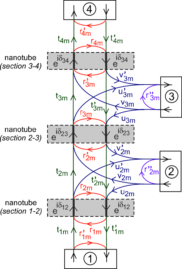
Figure 2: Scheme representing the notations used for the scattering amplitudes of channel $m$ in setups (a) and (b). The rectangles with full lines represent the different leads and the dashed rectangles represent the nanotube sections between those leads. We note $\delta_{jk}$ the phase shift acquired by electrons while propagating along the nanotube between contacts $j$ and $k$. At this stage, we use $\delta_{jk}=\delta_{kj}$, but we keep $t_{jm}\neq t_{jm}^{\prime}$, $u_{jm}\neq u_{jm}^{\prime}$, and $v_{jm}\neq v_{jm}^{\prime}$ for transparency of the calculation.

The phase shift $\delta_{jk}$ acquired by electrons along the CNT from contacts $j$ to $k$ can be considered as independent from $m$, with $\delta_{jk}=\delta_{kj}$Saito . In practice, $\delta_{12}$, $\delta_{23}$, and $\delta_{34}$ can be tuned using local gate voltage electrodes to change the electronic wavevector in the different CNT sections LocalGates . We will thus study the signals $G^{c}$, $V^{c}$, $MG$ and $MV$ as a function of these phases. The calculation of the voltage drop $V^{c}$ requires to determine $V_{3}^{c}$ and $V_{4}^{c}$ from $\left\langle I_{3}\right\rangle=\left\langle I_{4}\right\rangle=0$. This yields:

$$\frac{V^{c}}{V_{b}}=\frac{G_{41}G_{32}-G_{42}G_{31}}{G_{34}G_{43}-G_{33}G_{44}}$$ (3)

and

$$G^{c}/G_{K} =G_{11}+[G_{13}(G_{44}G_{31}-G_{41}G_{34})$$

$$+G_{14}(G_{41}G_{33}-G_{31}G_{43})]/[G_{34}G_{43}-G_{33}G_{44}]$$ (4)

Using the notations of Fig. 2, the elements $|S_{jk}^{m}|$ occurring in Eq. (3) through the coefficients $G_{jk}$ of Eq. (2) can be calculated as

$$\left|S_{41}^{m}\right|=\left|D_{m}^{-1}t_{1m}t_{2m}t_{3m}t_{4m}\right|$$ (5)

$$\left|S_{31}^{m}\right| =\left|D_{m}^{-1}t_{1m}t_{2m}\right|$$

$$\times\left|u_{3m}^{{}^{\prime}}+r_{4m}(t_{3m}v_{3m}^{\prime}-r_{3m}^{\prime}u_{3m}^{\prime})e^{i2\delta_{34}}\right|$$ (6)

$$\left|S_{42}^{m}\right| =\left|D_{m}^{-1}t_{3m}t_{4m}\right|$$

$$\times\left|v_{2m}+r_{1m}(t_{2m}u_{2m}-r_{2m}v_{2m})e^{i2\delta_{12}}\right|$$ (7)

$$S_{32}^{m}=S_{31}^{m}S_{42}^{m}/S_{41}^{m}$$ (8)

$$\left|S_{34}^{m}\right| =\left|D_{m}^{-1}t_{4m}^{\prime}\right|\times\left|v_{3m}^{\prime}(1-r_{1m}r_{2m}e^{i2\delta_{12}})\right.$$

$$+e^{i2\delta_{23}}(r_{2m}^{\prime}+r_{1m}e^{i2\delta_{12}}\left[t_{2m}t_{2m}^{\prime}-r_{2m}r_{2m}^{\prime}\right])$$

$$\times\left.(t_{3m}^{\prime}u_{3m}^{\prime}-r_{3m}v_{3m}^{\prime})\right|$$ (9)

and

$$\left|S_{43}^{m}\right| =\left|D_{m}^{-1}t_{4m}\right|\times\left|v_{3m}[1-r_{1m}r_{2m}e^{i2\delta_{12}}]\right.$$

$$+e^{i2\delta_{23}}[r_{2m}^{\prime}+r_{1m}e^{i2\delta_{12}}\left(t_{2m}t_{2m}^{\prime}-r_{2m}r_{2m}^{\prime}\right)]$$

$$\times\left.[t_{3m}u_{3m}-r_{3m}v_{3m}]\right|$$ (10)

with

$$D_{m} =[\left(1-r_{1m}r_{2m}e^{i2\delta_{12}}\right)\left(1-r_{2m}^{\prime}r_{3m}e^{i2\delta_{23}}\right)$$

$$\times\left(1-r_{3m}^{{}^{\prime}}r_{4m}e^{i2\delta_{34}}\right)]$$

$$-t_{2m}t_{2m}^{\prime}r_{1m}r_{3m}\left(1-r_{3m}^{{}^{\prime}}r_{4m}e^{i2\delta_{34}}\right)e^{i2(\delta_{12}+\delta_{23})}$$

$$-t_{3m}t_{3m}^{\prime}r_{2m}^{\prime}r_{4m}\left(1-r_{1m}r_{2m}e^{i2\delta_{12}}\right)e^{i2(\delta_{23}+\delta_{34})}$$

$$-t_{2m}t_{2m}^{\prime}t_{3m}t_{3m}^{\prime}r_{1m}r_{4m}e^{i2(\delta_{12}+\delta_{23}+\delta_{34})}$$ (11)

The missing coefficients $G_{33}$ and $G_{44}$ can be obtained from the above Eqs. using $G_{33}=-(G_{34}+G_{31}+G_{32})$ and $G_{44}=-(G_{43}+G_{41}+G_{42})$. For calculating $G^{c}$, one furthermore needs

$$\left|S_{14}^{m}\right|=\left|D_{m}^{-1}t_{1m}^{\prime}t_{2m}^{\prime}t_{3m}^{\prime}t_{4m}^{\prime}\right|$$ (12)

$$\left|S_{13}^{m}\right| =\left|D_{m}^{-1}t_{1m}^{\prime}t_{2m}^{\prime}\right|$$

$$\times\left|u_{3m}+r_{4m}e^{i2\delta_{34}}(t_{3m}^{\prime}v_{3m}-r_{3m}^{\prime}u_{3m})\right|$$ (13)

and

$$S_{11}^{m}-r_{1m}^{\prime} =D_{m}^{-1}t_{1m}t_{1m}^{\prime}e^{i2\delta_{12}}\{r_{2m}\left(1-r_{3m}^{\prime}r_{4m}e^{i2\delta_{34}}\right)$$

$$+e^{i2\delta_{23}}[r_{3m}+r_{4m}e^{i2\delta_{34}}(t_{3m}t_{3m}^{\prime}-r_{3m}r_{3m}^{\prime})]$$

$$\times[t_{2m}t_{2m}^{\prime}-r_{2m}r_{2m}^{\prime}]\}$$ (14)

The denominator $D_{m}$ accounts for multiple resonances inside the CNT. Figure 3 depicts some resonances $\mathcal{A}_{n}^{m}$, with $n\in[1,6]$, which can occur in limiting cases where $t_{2[3],m}=t_{2[3],m}^{{}^{\prime}}=0$ or $1$.

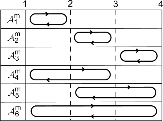
Figure 3: Scheme representing different resonances (noted $\mathcal{A}_{i}^{m}$) which can occur in setups (a) and (b) when $t_{2[3],m}=t_{2[3],m}^{{}^{\prime}}=0$ or $1$. The upper numbers indicate the position of contacts 1, 2, 3 and 4.

In the general case, Eq. (11) indicates that these different resonances are coupled. For $t_{2m}=t_{2m}^{{}^{\prime}}=0$, $G^{c}$ corresponds to the conductance of a two-terminals device, independent from $\delta_{23}$ and $\delta_{34}$, and $V^{c}$ vanishes. For $t_{2m}=t_{2m}^{{}^{\prime}}\neq 0$ and $t_{3m}=t_{3m}^{{}^{\prime}}=0$, $G^{c}$ depends on $\delta_{12}$ and $\delta_{23}$, but not on $\delta_{34}$, and $V^{c}$ still vanishes. Having a non-local signal $V^{c}\neq 0$ requires a direct CNT-CNT transmission at both contacts $2$ and $3$. It also requires that the four channels $m$ are not coupled to the leads in the same way. Indeed, from Eqs. (3) and (8), one can check that if all the $S_{jk}^{m}$ coefficients are independent from $m$, one finds $V^{c}=0$ due to the series structure of the device Baranger . Interestingly, a finite $V^{c}$ has already been obtained in a CNT connected to four normal-metal leadsMakarovski , which suggests that the $K$ and $K^{\prime}$ modes were not similarly coupled to those leads. In principle, such an asymmetry is also possible with ferromagnetic contacts.

IV.2 Parametrization of the lead/nanotube contacts

In the following, we assume that the top and bottom halves of the three terminals contacts $j\in\{2,3\}$ in Fig. 1 are symmetric. We furthermore take into account that the scattering matrix associated to each contact is invariant upon transposition, due to spin-conservationSC . This gives $t_{jm}=t_{jm}^{\prime}$, $r_{jm}=r_{jm}^{\prime}$, and $u_{jm}=u_{jm}^{\prime}=v_{jm}=v_{jm}^{\prime}$ for $j\in\{2,3\}$. In this case, on can check from Eqs. (5-14) that $G^{c}$ and $V^{c}$ depend only on six interfacial scattering phases, i.e. those of $r_{1m}$, $t_{2m}$, $r_{2m}$, $t_{3m}$, $r_{3m}$ and $r_{4m}$, which correspond to processes during which electrons remain inside the CNT simpl . For contacts $j\in\{2,3\}$, it is thus convenient to use the parametrization

$$t_{j(p,\sigma)}=\sqrt{T_{j,p}(1+\sigma P_{j,p})}e^{i(\varphi_{j,p}^{T}+\frac{\sigma}{2}\Delta\varphi_{j,p}^{T})}$$ (15)

$$r_{j(p,\sigma)} =\left[\sqrt{1-\left|t_{j(p,\sigma)}\sin[\phi_{j}^{(p,\sigma)}]\right|^{2}}\right.$$

$$+\left.\left|t_{j(p,\sigma)}\right|\cos[\phi_{j}^{(p,\sigma)}]\right]e^{i(\varphi_{j,p}^{R}+\frac{\sigma}{2}\Delta\varphi_{j,p}^{R})}$$ (16)

$$\left|u_{jm}\right|=\sqrt{1-\left|r_{jm}\right|^{2}-\left|t_{jm}\right|^{2}}$$ (17)

with

$$\phi_{j}^{(p,\sigma)}=\varphi_{j,p}^{R}-\varphi_{j,p}^{T}+\frac{\sigma}{2}(\Delta\varphi_{j,p}^{R}-\Delta\varphi_{j,p}^{T})$$

The above expressions depend on six real parameters $T_{j,p}$, $P_{j,p}$, $\varphi_{j,p}^{T}$, $\varphi_{j,p}^{R}$, $\Delta\varphi_{j,p}^{R}$ and $\Delta\varphi_{j,p}^{T}$param . In order to have unitary lead/CNT scattering matrices, on must use $0\leq T_{j,p}(1+\sigma P_{j,p})\leq 1$ andannul $\pi/2\leq\phi_{j}^{m}[2\pi]\leq 3\pi/2$. These conditions imply $0\leq|t_{jm}|^{2}\leq 1$, $0\leq|r_{jm}|^{2}\leq 1$ andsym $0\leq|u_{jm}|^{2}\leq 1/2$. For contacts $j\in\{1,4\}$, one can use

$$\left|t_{j}^{(p,\sigma)}\right|=\left|t_{j}^{{}^{\prime}(p,\sigma)}\right|=\sqrt{T_{j,p}(1+\sigma P_{j,p})}$$ (18)

and

$$\arg(r_{j}^{(p,\sigma)})=c_{p}\varphi_{j}^{R}+\frac{\sigma}{2}\Delta\varphi_{j,p}^{R}$$ (19)

with $c_{K(K^{\prime})}=\pm 1$. In Eq. (19), we have assumed $\sum_{p,\sigma}\arg(r_{1}^{(p,\sigma)})=0$ and $\sum_{p,\sigma}\arg(r_{4}^{(p,\sigma)})=0$, because, from Eqs. (5-14), these quantities only shift the variations of $G^{c}$, $V^{c}$, $MG$ and $MV$ with respect to $\delta_{12}$ and $\delta_{34}$, respectively. The parameters $P_{j,p}$, with $j\in\{1,2,3,4\}$, produce a spin-polarization of the transmission probabilities $|t_{j}^{m}|^{2}$. The parameters $\Delta\varphi_{j,p}^{R(T)}$ allow to take into account the Spin-Dependence of Interfacial Phase Shifts (SDIPS), which has already been shown to affect significantly the behavior of CNT spin-valvesCottet06a ; Cottet06b ; Sahoo . We will show below that the SDIPS also modifies the behavior of multi-terminal setups. Note that for $j\in\{2,3\}$, the parameters $\Delta\varphi_{p,j}^{R(T)}$ also contribute to the spin dependence of $|r_{jm}|^{2}$ and $|u_{jm}|^{2}$: the SDIPS and the spin-dependence of interfacial scattering probabilities are not independent in three-terminal contacts, due to the unitarity of scattering processes.

IV.3 Behavior of setup (a)

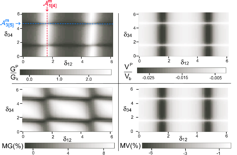
Figure 4: Signals $G^{P}$ (top left panel), $V^{P}$ (top right panel), $MG$ (bottom left panel), and $MV$ (bottom right panel) as a function of $\delta_{12}$ (horizontal axes) and $\delta_{34}$ (vertical axes) for a setup (a) with symmetric $K$ and $K^{\prime}$ channels. We have used $T_{1,K[K^{\prime}]}$ $=0.6$, $T_{2,K[K^{\prime}]}$ $=0.1$, $T_{(3)4,K[K^{\prime}]}$ $=0.3$, $P_{2[3],K[K^{\prime}]}$ $=0.4$, $\varphi_{1(4)}^{R}=0$, $\varphi_{2(3),K[K^{\prime}]}^{R}=\pi$, $\varphi_{2[3],K[K^{\prime}]}^{T}=0$, $\Delta\varphi_{2(3),K[K^{\prime}]}^{R\{T\}}=0$ and $\delta_{23}=\pi$. We have indicated the position of the resonances $\mathcal{A}_{1(4)}^{m}$ and $\mathcal{A}_{3(5)}^{m}$ with red and blue dashed lines, respectively.

We now consider setup (a), which has been frequently used in the MDI regime, for studying the spin accumulation effectJohnson ; Jedema ; Jedema2 ; Zaffalon ; Lou ; Tombros2 . We first assume that the $K$ and $K^{\prime}$ channels are coupled identically to the leads. This case is illustrated by Fig. 4, which shows the variations of $G^{P}$ (top left panel), $V^{P}$ (top right panel), $MG$ (bottom left panel) and $MV$ (bottom right panel) versus $\delta_{12}$ (horizontal axes) and $\delta_{34}$ (vertical axes). One can first notice that all these signals present strong variations with $\delta_{12}$ and $\delta_{34}$, due to quantum interferences occurring inside the CNT. In Fig. 4, $G^{P}(\delta_{12})$ presents peaks which correspond to the resonances $\mathcal{A}_{1}^{m}$ (see e.g. red dashed line), because we consider a case where $T_{2m}$ is weak (these peaks also correspond accidentally to the resonances $\mathcal{A}_{4}^{m}$, which are much broader). A more remarkable result is that $G^{P}(\delta_{34})$ presents antiresonances which correspond to $\mathcal{A}_{3}^{m}$ and $\mathcal{A}_{5}^{m}$ (see e.g. blue dashed line). This is a signature of the strongly non-local nature of current transport in this circuit: the electric signal measured in a given section of the CNT can be sensitive to resonances occurring in other sections of the CNT. We note that in Fig. 4, $\left|V^{P}\right|$ presents the same type of variations as $G^{P}$ with $\delta_{12}$ and $\delta_{34}$. In the general case, the resonances or antiresonances shown by the electric signals will not necessarily correspond to those defined in Fig. 3, due to the strong coupling between these different types of resonances. Importantly, we find that the $MG$ signal can be finite, contrarily to what happens in the MDI limit. Indeed, in Fig. 4, $MG$ can exceed $8\%$. We note that in Fig. 4, $MG$ presents minima approximately correlated with the maxima of $G^{P}$ in the $\delta_{12}$ direction, and with the minima of $G^{P}$ in the $\delta_{34}$ direction. In the case of a $S^{m}$ matrix independent from $m$, one finds $V^{c}=0$ (see section IV). By continuity, since we have used in Fig. 4 relatively low values for $P_{2[3],K[K^{\prime}]}$, no SDIPS and symmetric $K$ and $K^{\prime}$ channels, we find $\left|V^{P}\right|\ll V_{b}$. More precisely, a lowest order development with respect to $P_{2}$ and $P_{3}$ yields $V^{P}\sim-V^{AP}\sim\lambda P_{2}P_{3}$, with $\lambda\ll 1$ a function of the different system parameters. In these conditions, $MV$ presents the same type of variations as $V^{P}$ (one has $MV\sim 2V^{P}$). When the $K$ and $K^{\prime}$ modes are strongly asymmetric, it is possible to obtain a strong $\left|V^{P}/V_{b}\right|$ ratio for relatively low polarizations $P_{2[3],p}$. This case is illustrated by Fig. 5, where we have used $T_{1[4],K}\neq T_{1[4],K^{\prime}}$ and $\varphi_{1(4)}^{R}\neq 0$, so that $\mathcal{A}_{1[4]}^{(K,\sigma)}\neq\mathcal{A}_{1[4]}^{(K^{\prime},\sigma)}$ and $\mathcal{A}_{3[5]}^{(K,\sigma)}\neq\mathcal{A}_{3[5]}^{(K^{\prime},\sigma)}$. In this case, the variations shown by the different electric signals are more complicated than previously. However, we find $V^{P}\sim V^{AP}$, so that the amplitude of $MV$ remains comparable to that of Fig. 4.

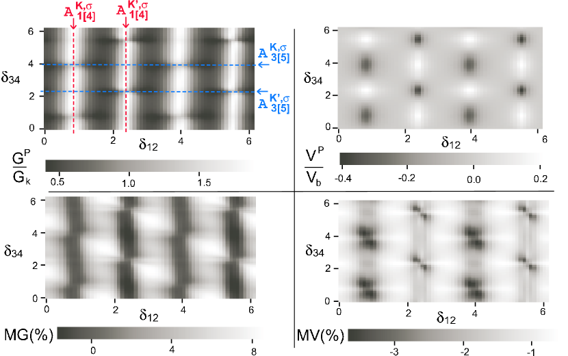
Figure 5: Signals $G^{P}$, $V^{P}$ , $MG$, and $MV$ as a function of $\delta_{12}$ and $\delta_{34}$, for a setup (a) with dissymmetric $K$ and $K^{\prime}$ channels. We have used $T_{1[4],K}=0.5$, $T_{1[4],K^{\prime}}=0.3$, $T_{2,K[K^{\prime}]}$ $=0.1$, $T_{3,K[K^{\prime}]}=0.3$, $P_{2[3],K[K^{\prime}]}$ $=0.4$, $\varphi_{2(3),K[K^{\prime}]}^{R}=\pi$, $\varphi_{2[3],K[K^{\prime}]}^{T}=0$, $\varphi_{1(4)}^{R}=\pi/2$, $\Delta\varphi_{2(3),K[K^{\prime}]}^{R\{T\}}=0$ and $\delta_{23}=\pi$. We have indicated the position of the resonances $\mathcal{A}_{1(4)}^{m}$ and $\mathcal{A}_{3(5)}^{m}$ with red and blue dashed lines, respectively.

We now discuss the signs of the different signals. We have already seen above that with the parameters of Fig. 4, one has $V^{P}>0$ and $V^{AP}<0$. In other conditions, it is possible to have $V^{P}<0$ and $V^{AP}>0$, or $V^{P}$and $V^{AP}$ both positive, or both negative (not shown). In the CFC model, the signs of $V^{P}$ and $V^{AP}$ are thus independent, whereas MDI models usually give opposite signs for $V^{P}$ and $V^{AP}$ (see e.g. Eq. (21) of Appendix A and Refs. Johnson2, ; Takahashi, ). Figure 5 illustrates that there exists sets of parameters such that the non-local voltage $V^{P}$ changes sign while sweeping $\delta_{12}$ or $\delta_{34}$ (this result is also true for $\delta_{23}$) SignChange . It is also possible to find sets of parameters such that $MV$ (not shown) and $MG$ (see Fig. 6, bottom left panel, full lines) change sign with $\delta_{12}$, $\delta_{23}$ or $\delta_{34}$.

We now briefly discuss the effects of the contacts polarizations. One can generally increase the amplitude of the magnetic signals by increasing $P_{j,p}$ (not shown), $\left|\Delta\varphi_{j,p}^{R}\right|$ (see Fig. 6, red full lines) and $\left|\Delta\varphi_{j,p}^{T}\right|$ (not shown). A strong SDIPS can split the resonances or antiresonances of the electric signals (not shown), like already found in the two-terminals $F$/CNT/$F$ caseCottet06a . Interestingly, in the case of a two-terminals $F$/CNT/$F$ device with a $K-K^{\prime}$ degeneracy and no SDIPS (using $1=F$, $2=F$ and no leads $3$ and $4$), Ref. Cottet06a, has found that the oscillations of $MG$ with $\delta_{12}$ are symmetric, and a finite SDIPS is necessary to break this symmetry. In contrast, in setup (a), the oscillations of $MG(\delta_{12})$ can be asymmetric in spite of the $K-K^{\prime}$ degeneracy and the absence of a SDIPS (see Fig. 6, bottom left panel).

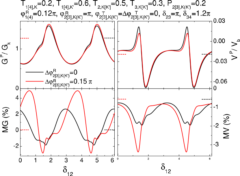
Figure 6: Signals $G^{P}$, $V^{P}$, $MG$, and $MV$ as a function of $\delta_{12}$ for setup (a). We consider a case with no SDIPS (black lines) and a case with a finite SDIPS (red lines corresponding to $\Delta\varphi_{2(3),K[K^{\prime}]}^{R}=0.15\pi$). We have used $T_{1[4],K}=0.2$, $T_{1[4],K^{\prime}}=0.6$, $T_{2,K[K^{\prime}]}$ $=0.5$, $T_{3,K[K^{\prime}]}=0.3$, $P_{2[3],K[K^{\prime}]}$ $=0.2$, $\varphi_{1(4)}^{R}=0.12\pi$, $\varphi_{2(3),K[K^{\prime}]}^{R}=\pi$, $\varphi_{2[3],K[K^{\prime}]}^{T}=\Delta\varphi_{2(3),K[K^{\prime}]}^{T}=0$, $\delta_{23}=\pi$ and $\delta_{34}=0.12\pi$. The full lines correspond to the CFC prediction (section IV), and the dotted lines to the IFC prediction (section V). The second does not depend on $\delta_{12}$. In the IFC case, the MG signal is hardly visible in this figure because it is of the order of 0.06%.

IV.4 Behavior of setup (b)

In setup (b), the types of resonances or antiresonances shown by the electric signals depend again on the value of the coupling between the different CNT sections. We will only highlight the most interesting specificities of setup (b), because it has many common properties with setup (a). Fig. 7 shows, with black [red] full lines, examples of $G^{P}(\delta_{12})$, $MG(\delta_{12})$, $V^{P}(\delta_{12})$, and $MV(\delta_{12})$ curves, for symmetric [asymmetric] $K$ and $K^{\prime}$ channels . Strikingly, in both cases, the magnetoconductance $MG$ between the $N$ leads 1 and 2 can be finite, although the two $F$ leads are located outside the classical current path. This is in strong contrast with the MDI limit. From Eqs. (3-8), the voltage difference $V^{c}$ vanishes if the scattering properties of contacts $1$ or $2$ are independent from the transverse index $p$, regardless of the scattering properties of contacts $3$ and $4$check . This leads to the paradoxical situation where a magnetic signal can be measured between the two $N$ leads but not between the two $F$ leads (see black full lines in Fig. 7). By continuity, when the $K-K^{\prime}$ asymmetry is not large at contacts 1 and 2, the amplitude of the signals $V^{P}$ and $MV$ measured between contacts $3$ and $4$ will remain very small. It is possible to obtain stronger amplitudes for $V^{c}$ and $MV$ in the opposite limit of strongly asymmetric $K$ and $K^{\prime}$ channels (see red full lines in Fig. 7, for which we have used $\varphi_{2,K}\neq\varphi_{2,K^{\prime}}$). With setup (b), is thus also possible to obtain magnetic signals in both $G^{c}$ and $V^{c}$, whereas $MG$ and $MV$ would vanish in the $MDI$ limit.

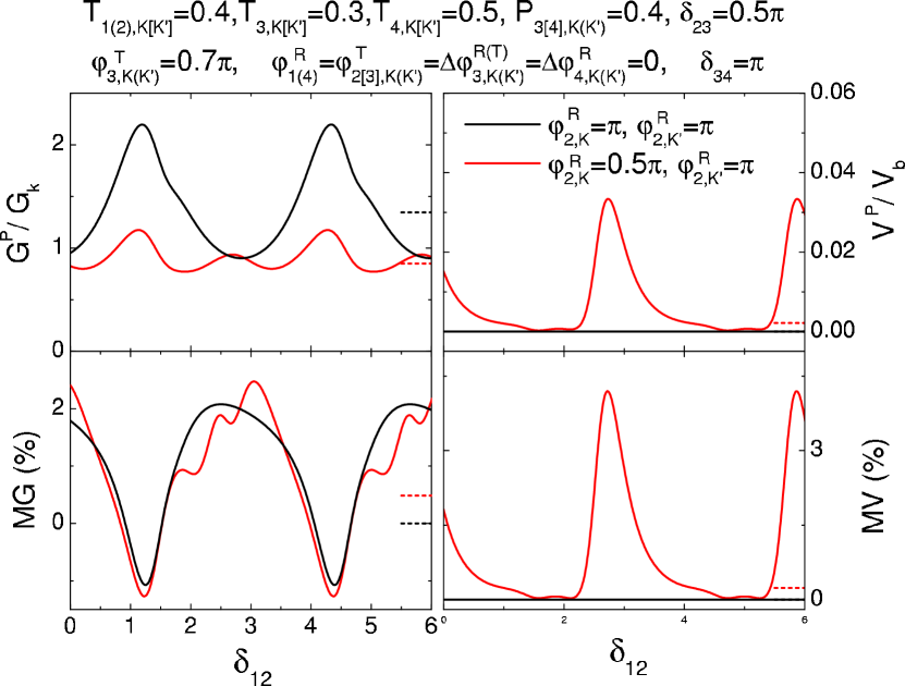
Figure 7: Signals $G^{P}$, $V^{P}$, $MG$, and $MV$ as a function of $\delta_{12}$, for setup (b). The black (red) lines correspond to the cases of $K$ and $K^{\prime}$ channels coupled identically (differently) to the contacts, i.e. $\varphi_{2,K}^{R}=\varphi_{2,K^{\prime}}^{R}=\pi$ ($\varphi_{2,K}^{R}=1.2\pi$, $\varphi_{2,K^{\prime}}^{R}=0.6\pi$). We have used $T_{1[2],K(K^{\prime})}=0.4$, $T_{3,K[K^{\prime}]}=0.3$, $T_{4,K[K^{\prime}]}=0.5$, $P_{3[4],K[K^{\prime}]}$ $=0.4$, $\varphi_{1(4)}^{R}=\varphi_{2(3),K[K^{\prime}]}^{T}=\Delta\varphi_{3,K[K^{\prime}]}^{R(T)}=\Delta\varphi_{4,K[K^{\prime}]}^{R}=0$, $\delta_{23}=\pi/2$ and $\delta_{34}=\pi$. The full lines correspond to the CFC prediction and the dotted lines to the IFC prediction. In the black case, the $MG$ signal vanishes in the IFC limit, and the $V^{P}$ and $MV$ signals vanish in both the IFC and CFC limits. The MG signal of the red case is hardly visible in the IFC limit because it is of the order of 0.03%.

IV.5 Comparison with the MDI limit

In this section, we summarize the most striking differences between the coherent four-channels (CFC) model of section IV and the MDI model of section III. For setup (b), the CFC model allows $V^{P}\neq 0$ and $MV\neq 0$ whereas one finds $V^{P}=0$ and $MV=0$ with the MDI model. Another remarkable result is that for both setups (a) and (b), the CFC model gives $G^{P}\neq G^{AP}$ whereas the MDI model imposes $G^{P}=G^{AP}$. The table in Fig. 1 summarizes these results.

V Incoherent four-channels limit

In order to determine whether the specific spin-dependent behavior of the CFC model is due to coherence or to the low number of channels, it is interesting to consider the incoherent four-channels (IFC) limit. If the phase relaxation length of the CNT is much shorter than the distance between the different contacts, the global transmission and reflection probabilities of setups (a) and (b) can be calculated by composing the scattering probabilities of the different contacts instead of the scattering amplitudesDatta . We have checked that this leads to replacing the scattering probabilities $\left|S_{\alpha\beta}^{m}(\{r_{jm},t_{jm},v_{jm},u_{jm},\delta_{ij}\})\right|^{2}$ occurring in Eqs.(1) and (2) by $S_{\alpha\beta}^{m}(\{\left|r_{jm}\right|^{2},\left|t_{jm}\right|^{2},\left|v_{jm}\right|^{2},\left|u_{jm}\right|^{2},0\})$. Importantly, this description remains intrinsically quantum since the channel quantization is taken into account. In Figs. 6 and 7, we show with black and red dotted lines the IFC values corresponding to the different CFC curves. We find that $G^{c}$, $V^{c}$, $MG$ and $MV$ do not depend anymore on the phases $\delta_{ij}$. However, $G^{P}\neq G^{AP}$ is still possible for setups (a) and (b). More precisely, we have checked analytically that using identical $K$ and $K^{\prime}$ modes leads tocheck $G^{P}=G^{AP}$, and we have checked numerically that $G^{P}\neq G^{AP}$ occurs in case of a $K$/$K^{\prime}$ asymmetry at one of the four contacts for setup (a), and at contacts 1 or 2 for setup (b). We can also obtain $V^{P}\neq 0$ and $MV\neq 0$ for setup (b) [and, more trivially, for setup (a)], with the same symmetry restrictions as for the CFC case (see table in Fig. 1). Therefore, having $V^{P}\neq 0$ and $MV\neq 0$ for setup (b), and $MG\neq 0$ for setups (a) and (b) is not a specificity the coherent case: using a very small number of transport channels already allows these properties. It is nevertheless important to notice that the values of $MG$ and $MV$ are strongly enhanced in the CFC case, due to resonance effects. Moreover, in the IFC case, the circuit is insensitive to the SDIPS, whereas in the coherent case, the SDIPS furthermore increases the amplitude of $MV$ and $MG$IFCnoSDIPS . At last, the coherent case presents the interest of allowing strong variations of the electric signals with the gate-controlled phases $\delta_{12}$, $\delta_{23}$ and $\delta_{34}$.

VI Discussion on first experiments

Reference Tombros, reports on a Single Wall Carbon Nanotube (SWNT) circuit biased like in Fig. 1, but with four ferromagnetic leads. A hysteretic $V^{c}$ has been measured by flipping sequentially the magnetizations of the two inner contacts. However, no conclusion can be drawn from this experiment, due to the lack of information on the conduction regime followed by the device. Reference Gunnar, reports on $V^{c}$ measurements for a setup (a) made with a SWNT. The authors of this Ref. have observed a finite $V^{c}$ which oscillates around zero while the back gate voltage of the sample is swept. This suggests that this experiment was in the coherent regime. However, the amplitude of $V^{c}$ was very low ($\max(\left|V^{c}/V_{b}\right|)\sim 0.01$), which indicates, in the framework of the scattering model, that the $K$ and $K^{\prime}$ modes were very close and the spin polarization of the contacts scattering properties very weak. It is therefore not surprising that these authors did not obtain a measurable $MV$ signal. Although setup (a) seems very popular in the nanospintronics community for historical reasons Johnson , we have shown above that setup (b) also highly deserves an experimental effort, as well as $MG$ measurements in general.

In this article, we have chosen to focus on the case of double mode quantum wires because this is adapted for describing CNT based devices, which are presently among the most advanced nanospintronics devices. However, technological progress might offer the opportunity to observe the effects depicted in this article in other types of nanowires, like e.g. semiconducting nanowires. Indeed, quantum interferences have already been observed in SiTilke and InAs quantum wiresDoh , and spin-injection has already been demonstrated in Si layers Jonker and InAs quantum dotsHamaya . One major difficulty may consist in reaching the few modes and fully ballisticZhou regime with these devices.

VII Conclusion

In this work, we have studied theoretically various circuits consisting of a carbon nanotube with two transverse modes, contacted to two normal metal leads and two ferromagnetic leads. Two contacts are used as source and drain to define a local conductance, and the two other contacts are left floating, to define a non-local voltage outside the classical current path. When the magnetizations of the two ferromagnetic contacts are changed from a parallel to an antiparallel configuration, we predict, in the local conductance and the non-local voltage, magnetic signals which are specific to the case of a system with a low number of channels. In particular, we propose an arrangement of the normal and ferromagnetic leads [setup (b)] which would give no magnetic response in the multichannel diffusive incoherent (MDI) limit, but which allows magnetic responses in both the local conductance and the non-local voltage in the two-modes regime. The more traditional arrangement [setup (a)] used for the study of the MDI limit also shows a qualitatively new behavior, i.e. a magnetic response in the local conductance. These specific magnetic behaviors are strongly reinforced in the coherent case, due to resonance effects occurring inside the nanotube, and also, possibly, due to the Spin-Dependence of Interfacial Phase Shifts. Our calculations pave the way to new experiments on non-local spin-transport in low-dimensional conductors.

We acknowledge discussions with H. U. Baranger and G. E. W. Bauer. This work was financially supported by the ANR-05-NANO-055 contract, the European Union contract FP6-IST-021285-2 and the C’Nano Ile de France contract SPINMOL.

VIII Appendix A: Discussion of the MDI limit with a resistors network

In this appendix, we discuss the MDI regime with an elementary but insightful resistors network model. When the electronic mean free path is much shorter than the spin-flip length, it is possible to define a spin-dependent electrochemical potential which obeys a local spin-dependent Ohm’s lawZutic . Thus, neglecting spin-flip scattering inside the CC, one can use the effective resistor network of Fig. 8 to describe the behaviors of setups (a) and (b) in the MDI limitValet ; Tombros . For completeness, we allow the four leads $j\in\{1,2,3,4\}$ to be ferromagnetic, with colinear magnetizations. The left (right) part of the resistors network corresponds to the up (down) spin channels.

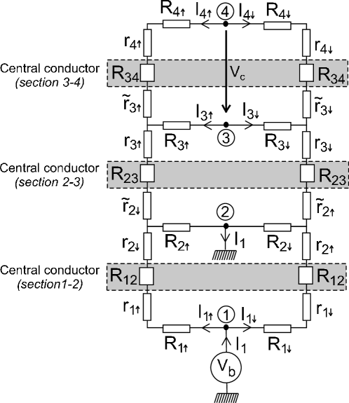
Figure 8: Resistors network used to describe the behavior of a one dimensional Central Conductor (CC) connected to four leads $j\in\{1,2,3,4\}$ in the MDI limit. The contact between lead $j$ and the CC is represented by the resistors $R_{j}^{\sigma}$, $r_{j}^{\sigma}$, and $\widetilde{r}_{j}^{\sigma}$. The section $j-k$ of the CC is modeled with the two resistors $R_{jk}$. When lead $j$ is not ferromagnetic, one must use $R_{j}^{\uparrow}=R_{j}^{\downarrow}$, $r_{j}^{\uparrow}=r_{j}^{\downarrow}$, and $\widetilde{r}_{j}^{\uparrow}=\widetilde{r}_{j}^{\downarrow}$

Due to intra-lead spin-flip scattering, electrons are in local equilibrium in lead $j$. This equilibration is described by the electrical connection of $\uparrow$ and $\downarrow$ channels at node $j$, which has an electric potential $V_{j}^{c}$. The section $j-k$ of the CC is modeled with the two resistors $R_{jk}$. The contact between lead $j$ and the CC is represented by the resistors $R_{j}^{\sigma}$, $r_{j}^{\sigma}$, and $\widetilde{r}_{j}^{\sigma}$. When lead $j$ is not ferromagnetic, one must use $R_{j}^{\uparrow}=R_{j}^{\downarrow}$, $r_{j}^{\uparrow}=r_{j}^{\downarrow}$, and $\widetilde{r}_{j}^{\uparrow}=\widetilde{r}_{j}^{\downarrow}$. The current flowing from lead $1$ to lead $2$ is $I_{1}^{c}=I_{1\uparrow}^{c}+I_{1\downarrow}^{c}$. Since leads $3$ and $4$ are floating, they supply the CC with spin currents which are perfectly equilibrated, i.e. $I_{j\uparrow}=-I_{j\downarrow}$ for $\alpha\in\{3,4\}$. We find

$$G^{c}=\mathcal{H}V_{b}/\mathcal{D}$$ (20)

and

$$V^{c}=\left(A_{34}^{\uparrow}-A_{34}^{\downarrow}\right)\left(B_{12}^{\uparrow}-B_{12}^{\downarrow}\right)V_{b}/\mathcal{R}_{23}\mathcal{H}$$ (21)

with

$$\mathcal{R}_{23}=\frac{R_{3}^{\uparrow}+R_{3}^{\downarrow}}{\sum\limits_{\sigma}\left(\mathcal{R}_{34}^{\sigma}-R_{3}^{\sigma}\right)}+\sum\limits_{\sigma}\left(\widetilde{r}_{2}^{\sigma}+r_{3}^{\sigma}+R_{23}\right)$$ (22)

$$\mathcal{H}=\sum\limits_{\sigma}\left(\mathcal{R}_{12}^{\sigma}+\alpha_{\sigma,\sigma}+\alpha_{\sigma,-\sigma}\right)$$ (23)

$$\mathcal{D}=\left(\mathcal{R}_{12}^{\uparrow}+\alpha_{\uparrow,\uparrow}\right)\left(\mathcal{R}_{12}^{\downarrow}+\alpha_{\downarrow,\downarrow}\right)-\alpha_{\uparrow,\downarrow}\alpha_{\downarrow,\uparrow}$$ (24)

$$2A_{34}^{\sigma}=\mathcal{R}_{34}^{\sigma}\left[(R_{3}^{\uparrow}+R_{3}^{\downarrow})/(\mathcal{R}_{34}^{\uparrow}+\mathcal{R}_{34}^{\downarrow})\right]-R_{3}^{\sigma}$$ (25)

$$B_{12}^{\sigma}=\left(\mathcal{R}_{12}^{\sigma}+\alpha_{\sigma,\sigma}+\alpha_{-\sigma,\sigma}\right)\left(\mathcal{R}_{12}^{-\sigma}-R_{2}^{-\sigma}\right)$$ (26)

$$\alpha_{\sigma,\sigma^{\prime}}=R_{2}^{\sigma}(\mathcal{R}_{12}^{\sigma^{\prime}}-R_{2}^{\sigma^{\prime}})/\mathcal{R}_{23}$$ (27)

and

$$\mathcal{R}_{jk}^{\sigma}=R_{j}^{\sigma}+\widetilde{r}_{j}^{\sigma}+R_{k}^{\sigma}+r_{k}^{\sigma}+R_{jk}$$ (28)

for $(j,k)\in\{1,2,3,4\}^{2}$. The value of $\mathcal{H}$ is independent from the contacts magnetic configuration, but $\mathcal{D}$ depends on the relative configuration of leads $1$ and $2$, so that $G^{P}\neq G^{AP}$ is possible provided leads $1$ and $2$ are ferromagnetic. In contrast, the value of $G^{c}$ is independent from the magnetization directions of leads $3$ or $4$ because, due to $I_{3(4)\uparrow}=-I_{3(4)\downarrow}$, the resistors $R_{3}^{\sigma}$, $r_{3}^{\sigma}$, $\widetilde{r}_{3}^{\sigma}$, $R_{4}^{\sigma}$ and $r_{4}^{\sigma}$ of Fig. 8 are connected in series with $R_{3}^{-\sigma}$, $r_{3}^{-\sigma}$, $\widetilde{r}_{3}^{-\sigma}$, $R_{4}^{-\sigma}$ and $r_{4}^{-\sigma}$ respectively. We conclude that for setups (a) and (b), one has $G^{P}=G^{AP}$ in the MDI limit. From Eq. (21), having $V^{P}\neq 0$ requires that at least one of the biased leads $1$ or $2$ is ferromagnetic (for the generation of a spin-accumulation), and at least one of the floating leads $3$ or $4$ is ferromagnetic (for the detection of this spin-accumulation). These conditions are fulfilled for setup (a), but not for setup (b). Importantly, these results will not be modified if a moderate intra-CC spin-flip scattering or the finite width of the contacts is taken into account, because both features can be modelled with a distributed array of resistors connecting the two spin branches, which will not change the spin symmetry of the model of Fig. 8.

References

- (1) C. P. Umbach, P. Santhanam, C. van Haesendonck, and R. A. Webb, Appl. Phys. Lett. 50, 1289 (1987).
- (2) A. Benoit, C. P. Umbach, R. B. Laibowitz, and R. A. Webb, Phys. Rev. Lett. 58, 2343 (1987); W. J. Skocpol, P. M. Mankiewich, R. E. Howard, L. D. Jackel, D. M. Tennant, and A. D. Stone, Phys. Rev. Lett. 58, 2347 (1987).
- (3) M. Johnson and R.H. Silsbee, Phys. Rev. Lett. 55, 1790 (1985)
- (4) F.J. Jedema, A. T. Filip and B. J. van Wees, Nature 410, 345 (2001).
- (5) F. J. Jedema, H. B. Heersche, A. T. Filip, J. J. A. Baselmans, B. J. van Wees, Nature 416, 713 (2002).
- (6) M. Zaffalon and B. J. van Wees, Phys. Rev. B 71, 125401 (2005).
- (7) X. Lou, C. Adelmann, S. A. Crooker, E. S. Garlid, J. Zhang, K. S. M. Reddy, S. D. Flexner, C. J. Palmstrom, and P. A. Crowell, Nature Phys. 3, 197 (2007).
- (8) N. Tombros, C. Jozsa, M. Popinciuc, H. T. Jonkman, B. J. van Wees, Nature 448, 571 (2007).
- (9) R.H. Silsbee, Bull. Magn. Reson. 2, 284 (1980).
- (10) W. Liang, M. Bockrath, D. Bozovic, J. H. Hafner, M. Tinkham and H. Park Nature 411, 665 (2001); M. R. Buitelaar, A. Bachtold, T. Nussbaumer, M. Iqbal, and C. Schönenberger, Phys. Rev. Lett. 88,156801 (2002); D. Mann, A. Javey, J. Kong, Q. Wang, H. Dai, Nano Lett. 3, 1541 (2003); J. Cao, Q. Wang, M. Rolandi, and H. Dai, Phys. Rev. Lett. 93, 216803 (2004); H.T. Man, I.J.W. Wever, A.F. Morpurgo, Phys. Rev. B 73, 241401(R) (2006); K. Grove-Rasmussen, H. I. Jørgensen, P. E. Lindelof, Physica E 40, 92 (2007); L. G. Herrmann, T. Delattre, P. Morfin, J.-M. Berroir, B. Plaçais, D. C. Glattli, and T. Kontos, Phys. Rev. Lett. 99, 156804 (2007).
- (11) A. Cottet, T. Kontos, S. Sahoo, H.T. Man, M.-S. Choi, W. Belzig, C. Bruder, A.F. Morpurgo and C. Schönenberger, Semicond. Sci. Technol. 21, S78 (2006).
- (12) A. Makarovski, A. Zhukov, J. Liu, and G. Finkelstein, Phys. Rev. B 76, 161405 (2007).
- (13) N. Tombros, S. J. van der Molen, and B. J. van Wees, Phys. Rev. B 73, 233403 (2006).
- (14) G. Gunnarsson, J. Trbovic, and C. Schönenberger, Phys. Rev. B 77, 201405(R) (2008).
- (15) Chéryl Feuillet-Palma et al., unpublished.
- (16) W. Liang, M. Bockrath, and H. Park, Phys. Rev. Lett. 88, 126801 (2002); B. Babic and C. Schönenberger, Phys. Rev. B 70, 195408 (2004); P. Jarillo-Herrero, J. Kong, H. S. J. van der Zant, C. Dekker, L. P. Kouwenhoven, and S. De Franceschi, Phys. Rev. Lett. 94, 156802 (2005); S. Moriyama, T. Fuse, M. Suzuki, Y. Aoyagi, and K. Ishibashi, Phys. Rev. Lett. 94, 186806 (2005); S. Sapmaz, P. Jarillo-Herrero, J. Kong, C. Dekker, L. P. Kouwenhoven, and H. S. J. van der Zant, Phys. Rev. B 71, 153402 (2005).
- (17) A. Cottet, T. Kontos, W. Belzig, C. Schönenberger and C. Bruder, Europhys. Lett. 74, 320 (2006).
- (18) A. Cottet and M.-S. Choi, Phys. Rev. B. 74, 235316 (2006).
- (19) S. Sahoo, T. Kontos, J. Furer, C. Hoffmann, M. Gräber, A. Cottet, and C. Schönenberger, Nature Phys. 1, 99, (2005).
- (20) T. Valet and A. Fert, Phys. Rev. B 48, 7099 (1993).
- (21) I. Zutic, J. Fabian and S. Das Sarma, Rev. Mod. Phys. 76, 323 (2004).
- (22) M. Büttiker, Phys. Rev. Lett. 57, 1761 (1986).
- (23) Physical properties of carbon nanotubes, R. Saito, G. Dresselhaus and M.S. Dresselhaus, Imperial College Press, London (1998).
- (24) N. Mason, M. J. Biercuk, and C. M. Marcus, Science 303, 655 (2004); M. R. Gräber, W. A. Coish, C. Hoffmann, M. Weiss, J. Furer, S. Oberholzer, D. Loss, and C. Schönenberger, Phys. Rev. B 74, 075427 (2006).
- (25) H.U. Baranger, Phys. Rev. B 42, 11479 (1990).
- (26) Spin-conservation allows to map the scattering description of each spin component onto a spinless problem. Time reversal symmetry in each of these spinless problems implies , and .
- (27) From Eq. (14), the phase of can also affect the signals and . However, since the scattering matrix of contact 1 is unitary, one finds . It is thus sufficient to use as a parameter.
- (28) The complete parametrization of the scattering matrices of contacts requires extra parameters , and such that and . However, one can check that, with the assumptions made in part IV.B, the signals and are independent from and for both setups (a) and (b).
- (29) For completeness, we point out that the condition on can be relaxed if .
- (30) For , one has because we assume that an electron arriving from contact enters the top and bottom portions of the CNT with the same probabilities.
- (31) We find that the sign changes of can already occur in the spin-degenerate case. Accordingly, a change of sign in has already been observed for a CNT with four normal metal leads, by sweeping the CNT back-gate voltageMakarovski .
- (32) We have checked analytically that this property is true even when the contacts 2 and 3 are spatially asymmetric i.e. .
- (33) S. Datta, Electronic Transport in Mesoscopic Systems, Cambridge University Press, Cambridge (1995).
- (34) In the IFC case, and are sensitive to the parameters through the reflection probabilities of contacts and , but not through the scattering phases.
- (35) M. Johnson and R.H. Silsbee, Phys. Rev. B 37, 5312 (1988).
- (36) S. Takahashi and S. Maekawa, Phys. Rev. B 67, 052409 (2003).
- (37) A. T. Tilke, F. C. Simmel, H. Lorenz, R. H. Blick , and J. P. Kotthaus, Phys. Rev. B 68, 075311 (2003).
- (38) Y.-J. Doh, A. L. Roest, E. P. A. M. Bakkers, S. De Franceschi, L. P. Kouwenhoven, cond-mat/arXiv:0712.4298
- (39) Berend T. Jonker, George Kioseoglou, Aubrey T. Hanbicki, Connie H. Li, Phillip E. Thompson, Nature Physics 3, 542 (2007).
- (40) K. Hamaya, M. Kitabatake, K. Shibata, M. Jung, M. Kawamura, K. Hirakawa, T. Machida, S. Ishida, Y. Arakawa, Appl. Phys. Lett. 91, 022107 (2007); K. Hamaya, S. Masubuchi, M. Kawamura, T. Machida, M. Jung, K. Shibata, K. Hirakawa, T. Taniyama, S. Ishida, Y. Arakawa, Appl. Phys. Lett. 90, 053108 (2007).
- (41) X. Zhou, S. A. Dayeh, D. Aplin, D. Wang, and E. T. Yu, Appl. Phys. Lett. 89, 053113 (2006).