Fractality of the non-equilibrium stationary states of open
volume-preserving systems: II. Galton boards

Abstract

Galton boards are models of deterministic diffusion in a uniform external field, akin to driven periodic Lorentz gases, here considered in the absence of dissipation mechanism. Assuming a cylindrical geometry with axis along the direction of the external field, the two-dimensional board becomes a model for one-dimensional mass transport along the direction of the external field. This is a purely diffusive process which admits fractal non-equilibrium stationary states under flux boundary conditions. Analytical results are obtained for the statistics of multi-baker maps modeling such a non-uniform diffusion process. A correspondence is established between the local phase-space statistics and their macroscopic counter-parts. The fractality of the invariant state is shown to be responsible for the positiveness of the entropy production rate.

I Introduction

Studying the statistical properties of simple mechanical models with strongly chaotic dynamics helps understanding the connection between deterministic motion at the microscopic scale and transport processes which occur at the macroscopic scales. This is of particular importance with regards to the irreversibility of thermodynamics and specifically the dynamical origins of the positiveness of entropy production.

Such a mechanical device was originally introduced by Sir Francis Galton in the form of an apparatus which provides a mechanical illustration of the Gaussian spreading of independent random events Galton1889 . The Galton board, also known as quincunx or bean machine mathworld , consists of an upright board with a periodic array of pegs upon which a charge of small shots is released. The particles are let to collide on the way downward, thus displaying a seemingly erratic motion through the successive rows of pegs, until they reach the bottom of the board, where they are stopped.

Provided the actual dynamics are sufficiently chaotic and dissipative, one can idealize individual paths as Bernoulli trials, whereby every collision event results into the pellets hopping down to the right or left of the pegs with equal probabilities. The number of steps in the trials is then specified by the number of the rows of pegs in the board. Under such conditions, the heaps of shots that form at the bottom of the board are expected to be distributed according to a binomial distribution and thus approximate a normal distribution.

Though Galton’s board was intended precisely as a mechanical illustration of this idealized model, the dynamics of the board are necessarily more intricate, in particular with regards to inelasticity of the collisions between pegs and pellets and the friction exerted by the board’s surface on the pellets. However if the collisions between the pellets and pegs were perfectly elastic and the board frictionless, the energy of every individual pellet would be conserved along its path. As a consequence, the kinetic energy would increase linearly with the distance separating the pellet position from the top of the board, where one can assume it was released with a specified velocity, which, for the sake of specializing the motion to a fixed energy shell, we assume to be equal in magnitudes for all pellets. Such a conservative Galton board is also referred to as idealized.

The remarkable property of conservative Galton boards is that a pellet’s motion is recurrent, which is contrary to what had until recently seemed to be a widespread consensus. In other words, however far a pellet goes in the direction of the external field, and consequently however large its kinetic energy becomes, it will come back to the top of the board with probability one. This property was proved by Chernov and Dolgopyat CD07a ; CD07b , who also showed, in accordance to previous heuristic arguments and numerical studies, that the presence of the external field affects the scaling law of positions and velocities so that a pellet’s speed scales according to $v(t)\sim t^{1/3}$ and its coordinate $x(t)\sim t^{2/3}$. They further found exact limit distributions for the rescaled velocity $t^{-1/3}v(t)$ and position $t^{-2/3}x(t)$.

Galton boards and related models have attracted much attention in the statistical physics community. In particular, Lorentz gases, which describe the motion of independent classical point particles in an array of fixed scattering disks, have been the subject of intensive investigations as models of diffusive transport of light tracer particles among heavier ones Lor1905 ; vB82 ; Det00 ; CC70 ; HKM74 . Lorentz gases have enjoyed a privileged status in the development of non-equilibrium statistical mechanics, which stems from the simplicity of its dynamics. By neglecting the recoil of heavy particles upon collision with the light tracer particles, one obtains a low-dimensional model that is amenable to a proper thermodynamical treatment while it retains important characteristics of genuine many-particle systems. This model has been studied with mathematical rigor and, in particular, the existence of a well-defined diffusion coefficient has been proved rigorously under certain conditions BS80 . Furthermore, in the last decades, and in the context of molecular dynamics simulations of non-equilibrium systems Hoo86 ; EM90 , several versions of the Lorentz gas model have been considered, including the Gaussian thermostated Lorentz gas in the presence of a uniform external field MH87 , for which the Einstein relation between the coefficients of electrical conductivity and diffusion has been proved CELS93 .

The reason for the initial success of the Lorentz gas was its use by Lorentz Lor1905 , elaborating on Drude’s theory of electrical and thermal conduction Dru1900 ; Mer76 , for the sake of deriving the Wiedemann-Franz law, which predicts the temperature dependence of the ratio between heat and electrical conductivities in metals. In this framework, the computation of the electrical conductivity assumes that the external field is weak enough that the tracer particle velocity magnitude is constant. Thus the diffusion coefficient is homogeneous and essentially given by the product of the particle’s mean free path and (thermal) velocity.

In a conservative diffusive system acted upon by an external field, the situation is different in that the external field causes the acceleration of particles and induces a velocity-dependent diffusion coefficient. Nevertheless such a system bears strong analogies with the field free diffusive case.

It is our purpose to investigate this analogy by comparing the statistical properties of Galton boards to that of periodic Lorentz gases. The latter were studied in a first paper BGGi , where we discussed the fractality of the non-equilibrium stationary states of open Lorentz gases under flux boundary conditions, i. e. a slab of finite extension with its two boundaries in contact with particle reservoirs with differing injection rates. Under such boundary conditions, the Lorentz gas sustains a steady current of mass which induces a constant rate of entropy production.

In BGGi , we established the connection between this production of entropy and the fractality of the stationary states of open Lorentz gases. In this follow-up paper, we extend these results to Galton boards and related models. In particular, we develop a discrete random walk model that mimics the collision dynamics of Galton boards and associate to it a multi-baker map with energy, similar to models introduced in TG99 ; TG00 . The specificity of our model is that the transition rates vary with the sites’ indices, reflecting the property of the conservative Galton board that deflection of tracers by the external field is more likely to occur when their kinetic energies are small in comparison to their potential energies. We derive the analytic expression of the non-equilibrium stationary states of this multi-baker map and show that its cumulative measures are characterized by nowhere differentiable continuous functions similar to the Takagi function of the non-equilibrium stationary state of the usual multi-baker map TG95 . This allows us to compute the entropy associated to such non-equilibrium stationary states and thus obtain an analytic derivation of the rate of entropy production, which, within our formalism, finds its origin in the fractality of the non-equilibrium stationary state, in agreement with the results presented in BGGi for the field free case.

The paper is organized as follows. Galton boards are presented in Sec. II. The connection to the phenomenology of diffusion in an external field, described in Sec. II.1, is established for both closed and open systems, whose statistical properties are considered in Sec. II.2. In Sec. II.3 we discuss the occurrence of elliptic islands in the Galton board’s dynamics, i.e. the stabilization of periodic orbits, and provide conditions under which we can assume the system to be fully hyperbolic. This regime is studied numerically, first under equilibrium setting in Sec. II.4, and then under non-equilibrium setting in Sec. II.5, where we demonstrate the fractality of the invariant measure. In Sec. III, we introduce the forced multi-baker map, which mimics the collision dynamics of the Galton board and analyze its statistics in Sec. III.1. The entropy production rate of the non-equilibrium stationary state is computed in Sec. III.2. We end with conclusions in Sec. IV.

II Galton board

The Galton board is similar to a periodic Lorentz gas in a uniform field. We consider a two-dimensional cylinder of length $L=Nl$ and height $\sqrt{3}l$, with disks $\mathbb{D}_{n}$, $0\leq n\leq 2N$, of radii $\sigma$, $\sqrt{3}/4<\sigma/l<1/2$, placed on a hexagonal lattice structure. The centers of the disks take positions

$$(x_{n},y_{n})=\left\{\begin{array}[]{l@{\quad}l}(nl/2,0)\,,&n\,\mathrm{odd},\\ (nl/2,\pm\sqrt{3}l/2)\,,&n\,\mathrm{even},\end{array}\right.$$ (1)

where we identify the disks $y=\pm\sqrt{3}l/2$. The cylindrical region around disk $\mathbb{D}_{n}$ is defined as

$$\mathbb{I}_{n}=\big{\{}(x,y)\ |\ (n-1/2)l/2\leq x\leq(n+1/2)l/2\big{\}}.$$ (2)

Thus the interior of the cylinder, where particles propagate freely is made up of the union $\cup_{n=-N}^{N}\mathbb{I}_{n}\setminus\mathbb{D}_{n}$.

The associated phase space, defined on a constant energy shell, is $\mathbb{C}=\cup_{n=-N}^{N}\mathbb{C}_{n}$, where $\mathbb{C}_{n}=\mathbb{S}^{1}\otimes[\mathbb{I}_{n}\setminus\mathbb{D}_{n}]$ and the unit circle $\mathbb{S}^{1}$ represents all possible velocity directions. Particles are reflected with elastic collision rules on the border $\partial\mathbb{C}$, except at the external borders, corresponding to $x=0,L$, where they get absorbed. Points in phase-space are denoted by $\Gamma=(x,y,v_{x},v_{y})$, and trajectories by $\Phi^{t}\Gamma$, with $\Phi^{t}$ the flow associated to the dynamics of the Galton board.

The collision map takes the point $\Gamma=(x,y,v_{x},v_{y})\in\partial\mathbb{C}$ to $\Phi^{\tau}\Gamma=(x^{\prime},y^{\prime},v_{x}^{\prime},v_{y}^{\prime})\in\partial\mathbb{C}$, where $\tau$ is the time that separates the two successive collisions with the border of the Lorentz channel $\partial\mathbb{C}$, and $(v_{x}^{\prime},v_{y}^{\prime})$ is obtained from $(v_{x},v_{y})$ first by propagation under the uniform accelaration until the instant of collision, and then applying the usual rules of specular collisions. Given that the energy $E$ is fixed, the collision map operates on a two-dimensional surface, which, when the collision takes place on disk $n$, is conveniently parameterized by the Birkhoff coordinates $(\phi_{n},\xi_{n})$, where $\phi_{n}$ specifies a generalized angle variable along the border of disk $n$, to be determined in Sec. II.4, and $\xi_{n}$ is the sinus of the angle that the particle velocity makes with respect to the outgoing normal to the disk after the collision.

The external field is uniform and directed along the positive $x$ direction, so that particles accelerate as they move along the axis of the channel, in the direction of the external field. There is no dissipative mechanism and energy is conserved along the Galton board trajectories.

In this system, as opposed to typical billiards, the energy, denoted $E$, can be both kinetic and potential. As the particle moves along the direction of the channel axis, it looses potential energy and gains kinetic energy, according to the energy conservation $E=(v_{x}^{2}+v_{y}^{2})/2-\epsilon x$, where $\epsilon$ denotes the amplitude of the external field. Conversely, the particle looses kinetic energy and gains potential energy as it moves in the direction opposite to the external field.

Assuming $E\geq 0$, the boundaries of the system are placed at $x=0$ and $x=L$, reflecting the impossibility for a trajectory to gain potential energy beyond the zero kinetic energy level. When $E=0$, trajectories turn around at $x\geq 0$ when the $x$ component of the velocity annihilates, whereas when $E>0$, depending on the choice of boundary conditions, particles can be either reflected or absorbed when they reach $x=0$.

The trajectory between two successive elastic collisions with the disks is now parabolic, according to $x(t)=x(0)+v_{x}(0)t+\epsilon t^{2}/2$, whereas the vertical motion is uniform $y(t)=y(0)+v_{y}(0)t$. The amplitude of the external field $\epsilon$ can be set to unity by an appropriate rescaling of the momenta and time variable: $v\to v/\sqrt{\epsilon}$ and $t\to t\sqrt{\epsilon}$. Correspondingly, the energy has the units of length.

We can thus write the velocity amplitude as a function of the $x$ coordinate,

$$v(x)=\sqrt{2(E+x)}.$$ (3)

In particular, the velocity amplitude at $x=0$ is $v(0)=\sqrt{2E}$. We will assume that the energy takes half integer values of the cell widths $l$, so that the kinetic energy takes half integer values at the horizontal positions of the disks along the channel, i.e at $x$’s which are half integer multiples of $l$.

The system is shown in Fig. 1 with absorbing boundary conditions at $x=0$ and $L$. Note that trajectories are seen to bend along the field only so long as the velocity is small enough that the action of the field is noticeable. Otherwise the trajectory looks much like that of the Lorentz channel in the absence of external field. The time scales are however different.

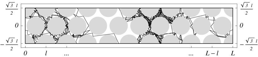
Figure 1: Cylindrical Galton board with a non-vanishing external field and the energy $E=0$. A trajectory is released at zero velocity at $x=0$, and falls along the external field until it collides a first time with a disk. It then wanders around, coming back close to $x=0$ once, after which it moves further along the channel until it reaches the border at $x=L$. To compute the successive collision events, the numerical integration scheme uses an exact quartic equation solver based on the Galois formula WQu .

II.1 Phenomenology

One often reads in the literature that Galton boards, or equivalently periodic Lorentz gases in a uniform external field, do not have a stationary state. This is however a confusing statement since the existence of the stationary state has nothing to do with the presence of the external field. Rather, it is a matter of boundary conditions.

Just as with the usual Lorentz gas, when an external forcing is turned on, a stationary state is reached so long as one specifies the boundary conditions. The reason for much of the confusion associated to this problem is, according to our understanding, that one cannot consider periodic boundary conditions along the direction of the field since they would violate the conservation of energy. One can however consider both reflecting and absorbing boundary conditions for the extended system. The nature of the stationary state, whether equilibrium or non-equilibrium, depends on the choice of boundary conditions.

A phenomenological diffusion equation can be obtained for the motion along the axis of the cylindrical channel, which corresponds to the direction of the external field.

In the presence of an external field, the diffusion process is a priori biased, so that the Fokker-Planck equation of diffusion reads

$$\partial_{t}\mathcal{P}(X,t)=\partial_{X}[\mathcal{D}(X)\partial_{X}\mathcal{P}(X,t)+\mathcal{M}(X)\mathcal{P}(X,t)]\,.$$ (4)

Here $X$ denotes a macroscopic position, associated to the projection along the axis direction of a given phase-space region $\mathbb{I}_{n}$ of the Galton board, taken in the continuum limit.

According to Einstein’s argument, the diffusion coefficient $\mathcal{D}(X)$ is connected to the mobility coefficient $\mathcal{M}(X)$ by the condition that Eq. (4) admits the equilibrium state $\mathcal{P}_{\mathrm{eq}}(X)$ as a solution which annihilates the mean current:

$$\mathcal{D}(X)\partial_{X}\mathcal{P}_{\mathrm{eq}}(X)+\mathcal{M}(X)\mathcal{P}_{\mathrm{eq}}(X)=0\,.$$ (5)

At the microscopic level, letting $\Gamma$ denote a phase point in $2d$ dimensions with velocity amplitude $v$ and position $x$ with respect to the direction of the external field, the equilibrium state is the microcanonical state i. e.

$$\rho_{\mathrm{eq}}(\Gamma)\propto\delta\left(E-\frac{v^{2}}{2}+x\right)\,,$$ (6)

Integrating this equilibrium phase-space density over cells $\mathbb{C}_{n}$ and taking the continuum limit $l\to 0$ and $n\to\infty$ with the macroscopic position variable $X=nl/2$ fixed, we obtain the macroscopic equilibrium density $\mathcal{P}_{\mathrm{eq}}(X)$,

$$\mathcal{P}_{\mathrm{eq}}(X)dX = \lim_{\stackrel{{\scriptstyle l\to 0}}{{n\to\infty}}}\int_{\mathbb{C}_{n}}d\Gamma\rho_{\mathrm{eq}}(\Gamma)\,,$$ (7)

$$\propto \lim_{\stackrel{{\scriptstyle l\to 0}}{{n\to\infty}}}\int_{\mathbb{C}_{n}}d\Gamma\delta\left(E-\frac{v^{2}}{2}+x\right)\,,$$

$$\propto \lim_{l\to 0}l\int dv\,v^{d-1}\delta\left(E-\frac{v^{2}}{2}+X\right)\,.$$

Identifying the length increments $dX=l$, and carrying out the velocity integration, we arrive to the expression of the equilibrium density

$$\mathcal{P}_{\mathrm{eq}}(X)=\mathcal{N}[2(E+X)]^{\frac{d-2}{2}}\,,$$ (8)

where $\mathcal{N}$ is a normalization factor. Inserting this expression into Eq. (5), we obtain the relation between the mobility and diffusion coefficients,

$$\mathcal{M}(X)=-\frac{d-2}{2}\frac{\mathcal{D}(X)}{E+X}\,.$$ (9)

The diffusion coefficient, on the other hand, is proportional to the magnitude of the position-dependent velocity, $V(X)=\sqrt{2(E+X)}$. This is a transposition of the corresponding result for the usual field free periodic Lorentz gas, where the tracer’s velocity has constant magnitude. In the Galton board, given an energy $E$ identical for all the tracer particles, the velocities $V(0)=\sqrt{2E}$ at $X=0$ are identical for all particles, growing with $X>0$, due to the uniform force of unit amplitude acting along that direction. We can therefore write

$$\mathcal{D}(X)=\mathcal{D}_{0}\sqrt{1+\frac{X}{E}}$$ (10)

Notice the normalization so chosen that the diffusion coefficient at $X=0$ reduces to $\mathcal{D}_{0}$. Equation (10) can be thought of as a transposition of the argument by Machta and Zwanzig MZ83 who provided an analytical expression of the diffusion coefficient for the periodic Lorentz gas, based upon a random walk approximation. This approximation indeed carries over to the Galton board. Provided energy is conserved, the velocity of a tracer particle increases as it moves along the direction of the external field. Thus, provided the periodic cells have sizes small enough that velocities remain approximately constant within each cell, the Machta-Zwanzig argument tells us that the diffusion coefficient is simply multiplied by a factor which accounts for the position-dependent velocity. Hence the expression (10).

Plugging Eq. (10) into (9), we obtain the expression of the mobility,

$$\mathcal{M}(X)=-\frac{d-2}{2}\frac{\mathcal{D}_{0}}{E\sqrt{1+\frac{X}{E}}}\,.$$ (11)

Remarkably, the mobility coefficient vanishes for a two-dimensional billiard. In this case, the Fokker-Planck equation (4) therefore simplifies to

$$\partial_{t}\mathcal{P}(X,t)=\partial_{X}[\mathcal{D}(X)\partial_{X}\mathcal{P}(X,t)]\,.$$ (12)

An equivalent equation was derived by Chernov and Dolgopyat in CD07a . This is a diffusive equation without a drift and describes the recurrent motion of the two-dimensional Galton board trajectory at the macroscopic scale. In contrast, we notice that the Fokker-Planck equation (4) associated to a three-dimensional version of the conservative Galton board has a non-vanishing mobility coefficient (11) and therefore retains a drift term.

In the sequel we will assume $E>0$ so as to avoid the singularities that come with zero velocity trajectories.

We notice, on the one hand, that reflection at the boundaries (RBC) induces an equilibrium state of Eq. (12) with constant density,

$$\mathcal{P}(X)=1,\quad(\mathrm{RBC})\,.$$ (13)

Flux boundary conditions (FBC), on the other hand, viz.

$$\left\{\begin{array}[]{c}\mathcal{P}(0)\equiv\mathcal{P}_{-},\\ \mathcal{P}(L)\equiv\mathcal{P}_{+},\end{array}\right.$$ (14)

admit the stationary state

$$\mathcal{P}(X)=C_{0}+C_{1}\sqrt{1+X/E},\quad(\mathrm{FBC})\,.$$ (15)

The coefficients $C_{0}$ and $C_{1}$ are determined by the boundary conditions at $X=0$ and $X=L$, Eq. (14):

$$C_{0} = \frac{\mathcal{P}_{-}\sqrt{1+L/E}-\mathcal{P}_{+}}{\sqrt{1+L/E}-1},$$ (16)

$$C_{1} = \frac{\mathcal{P}_{+}-\mathcal{P}_{-}}{\sqrt{1+L/E}-1}.$$ (17)

In terms of $\mathcal{P}_{\pm}$, we can rewrite Eq. (15) as

$$\mathcal{P}(X)=\mathcal{P}_{-}+(\mathcal{P}_{+}-\mathcal{P}_{-})\frac{\sqrt{E+X}-\sqrt{E}}{\sqrt{E+L}-\sqrt{E}}\,.$$ (18)

Given rates $\mathcal{P}_{-}\neq\mathcal{P}_{+}$, the current associated to the non-equilibrium stationary state is constant and, according to Fick’s law, equal to

$$\mathcal{J} = -\mathcal{D}(X)\partial_{X}\mathcal{P}(X)\,,$$ (19)

$$= -\frac{\mathcal{D}_{0}}{2E}\frac{\mathcal{P}_{+}-\mathcal{P}_{-}}{\sqrt{1+L/E}-1}\,.$$

The corresponding local rate of entropy production is given according to the usual formula, by the product of the mass current (19) and the associated thermodynamic force GND03 ,

$$\frac{d_{\mathrm{i}}\mathcal{S}(X)}{dt} = \mathcal{D}(X)\frac{[\partial_{X}\mathcal{P}(X)]^{2}}{\mathcal{P}(X)}.$$ (20)

II.2 Discretized Process

The deterministic models we consider are to be analyzed in terms of return maps, which involves a discretization of both time and length scales. We consider this problem in some detail, as it will be useful for the sake of defining a discrete process associated to the Galton board.

Let the discretized time and length scales be determined according to $t=k\tau$ and $X=nl$. Collision rates are proportional to the velocity, which brings in a factor $\sqrt{1+nl/E}$ after we time discretize Eq. (12),

$$\frac{1}{\tau}\sqrt{1+\frac{nl}{E}}\Big{[}\mathcal{P}(nl,k\tau+\tau)-\mathcal{P}(nl,k\tau)\Big{]}$$

$$= \frac{1}{l^{2}}\Big{\{}\mathcal{D}(nl+l/2)\mathcal{P}(nl+l,k\tau)+\mathcal{D}(nl-l/2)\mathcal{P}(nl-l,k\tau)-[\mathcal{D}(nl+l/2)+\mathcal{D}(nl-l/2)]\mathcal{P}(nl,k\tau)\Big{\}}\,.$$

We let

$$\mu_{n}(k)\equiv\sqrt{1+\frac{nl}{E}}\mathcal{P}(nl,k\tau)$$ (22)

be the collision frequency on the Poincaré surface at position $X=nl$, and introduce a diffusion coefficient associated to the discrete process,

$$D(n)\equiv\frac{\tau}{l^{2}}\mathcal{D}(nl)\,.$$ (23)

It is convenient to set $E\equiv(2n_{0}+1)l/2$, for some positive integer $n_{0}$.

Equation (II.2) thus transposes to the evolution

$$\mu_{n}(k+1)=\left[1-\frac{D(n+1/2)}{\sqrt{1+\frac{2n}{2n_{0}+1}}}-\frac{D(n-1/2)}{\sqrt{1+\frac{2n}{2n_{0}+1}}}\right]\mu_{n}(k)+\frac{D(n+1/2)}{\sqrt{1+\frac{2(n+1)}{2n_{0}+1}}}\mu_{n+1}(k)+\frac{D(n-1/2)}{\sqrt{1+\frac{2(n-1)}{2n_{0}+1}}}\mu_{n-1}(k)\,.$$ (24)

Written under the form

$$\mu_{n}(k+1)=s_{n-1}^{+}\mu_{n-1}(k)+s_{n}^{0}\mu_{n}(k)+s_{n+1}^{-}\mu_{n+1}(k)\,,$$ (25)

Eq. (24) is seen to be the Frobenius-Perron equation of the Markov process

$$n\longrightarrow\left\{\begin{array}[]{c@{\quad}c@{\:}c}n-1,&\hfil\>&s_{n}^{-}\,,\\ n,&\mathrm{with\ probability}\hfil\>&s_{n}^{0}\,,\\ n+1,&\hfil\>&s_{n}^{+}\,.\end{array}\right.$$ (26)

As opposed to a symmetric random walk, the probabilities $s_{n}^{-}$, $s_{n}^{0}$ and $s_{n}^{+}$ are asymmetric and depend on the site index,

$$\begin{array}[]{lcl}s_{n}^{-}&=&\frac{D(n-1/2)}{\sqrt{1+\frac{2n}{2n_{0}+1}}}\,,\\ s_{n}^{+}&=&\frac{D(n+1/2)}{\sqrt{1+\frac{2n}{2n_{0}+1}}}\,,\\ s_{n}^{0}&=&1-s_{n}^{-}-s_{n}^{+}\,.\end{array}$$ (27)

In these expressions, $n$ is assumed to be a positive integer, $0\leq n\leq N$. From Eq. (10), the diffusion coefficient may be written $D(n)=D_{0}\sqrt{1+\frac{2n}{2n_{0}+1}}$, where $D_{0}=\tau/l^{2}\mathcal{D}_{0}$, from which it follows that

$$s_{n}^{\pm}=D_{0}\sqrt{1\pm\frac{1}{2(n_{0}+n)+1}}\,.$$ (28)

It is straightforward to check that the stationary state of Eq. (25) is independent of $D_{0}$, and can be written under the form

$$\mu_{n}\equiv\lim_{k\to\infty}\mu_{n}(k)=\sqrt{\frac{2(n_{0}+n)+1}{2n_{0}+1}}P_{n},$$ (29)

where $P_{n}$ is the discretized stationary state of the Fokker-Planck equation (12),

$$P_{n}\Big{[}\sqrt{n_{0}+n+1}+\sqrt{n_{0}+n}\Big{]}$$

$$=P_{n+1}\sqrt{n_{0}+n+1}+P_{n-1}\sqrt{n_{0}+n}\,.$$

We note that the latter equation implies that $\sqrt{n_{0}+n}(P_{n}-P_{n-1})\equiv\alpha$ is constant. We can therefore write

$$P_{n} = P_{n-1}+\frac{\alpha}{\sqrt{n_{0}+n}}\,,$$ (31)

$$= P_{0}+\alpha\sum_{i=0}^{n}(n_{0}+i)^{-1/2},$$

$$= P_{0}+\alpha\Big{(}H_{n+n_{0}}^{\frac{1}{2}}-H_{n_{0}}^{\frac{1}{2}}\Big{)}\,,$$

where $H_{n+n_{0}}^{\frac{1}{2}}$ denotes the Harmonic number, $H_{n}^{\frac{1}{2}}=\sum_{j=1}^{n}j^{-1/2}$ Hnum . Letting $n=N$ in Eq. (31), $Nl=L$, and writing the boundary conditions $P_{0}\equiv P_{-}$ and $P_{N}\equiv P_{+}$, we obtain the expression of $\alpha$, $\alpha=(P_{+}-P_{-})/(H_{N+n_{0}}^{\frac{1}{2}}-H_{n_{0}}^{\frac{1}{2}})$. Therefore $P_{n}$ can be expressed as

$$P_{n}=P_{-}+(P_{+}-P_{-})\frac{H_{n+n_{0}}^{\frac{1}{2}}-H_{n_{0}}^{\frac{1}{2}}}{H_{N+n_{0}}^{\frac{1}{2}}-H_{n_{0}}^{\frac{1}{2}}}.$$ (32)

The connection to the continuous case and, in particular, to Eq. (18) is now straightforward. Indeed, the ratio of differences of Harmonic functions become integrals when $l\to 0$

$$\frac{H_{n+n_{0}}^{\frac{1}{2}}-H_{n_{0}}^{\frac{1}{2}}}{H_{N+n_{0}}^{\frac{1}{2}}-H_{n_{0}}^{\frac{1}{2}}}$$

$$= \frac{\frac{l}{\sqrt{E+l/2}}+\frac{l}{\sqrt{E+3l/2}}+\dots+\frac{l}{\sqrt{E+l/2+nl}}}{\frac{l}{\sqrt{E+l/2}}+\frac{l}{\sqrt{E+3l/2}}+\dots+\frac{l}{\sqrt{E+l/2+Nl}}}\,,$$

$$\to \frac{\int_{E}^{E+X}dx/\sqrt{x}}{\int_{E}^{E+L}dx/\sqrt{x}}=\frac{\sqrt{E+X}-\sqrt{E}}{\sqrt{E+L}-\sqrt{E}}\,,$$

where the limit assumes $l\to 0$ with $E$ constant and thus $n_{0}\gg 1$. In this case we have $P_{n}\to\mathcal{P}(X=nl)$.

II.3 Elliptic Islands

Prior to turning to the stationary states of Galton boards, whether equilibrium or non-equilibrium, we mention the possible lack of ergodicity of the Galton board. The external field can indeed stabilize periodic orbits when the kinetic energy is not too large. Figure 2 shows such an example. In this case, elliptic islands co-exist with chaotic trajectories, as seen in Fig. 3.

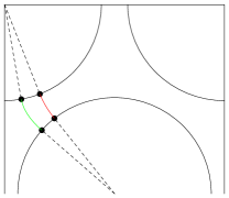
Figure 2: (Color online) The external field induces a bifurcation such that the simple periodic orbit bouncing off two neighboring disks at normal angles is replaced by two such orbits. In this situation where $E=0$, which corresponds to a vanishing kinetic energy on the left border, one of these two periodic orbits is stable (to the left) and the other one unstable (to the right). The stability of the periodic orbit is quickly lost as $E$ is increased.

Figure 3: Elliptic islands around the stable periodic orbit shown in Fig. 2: (Top) disk on the upper left corner; (Bottom) central disk. The phase-space coordinates used here (not the appropriate Birkhoff coordinates) are $\phi$, the angle around the corresponding disk, and $\xi$ the sinus of the velocity angle measures with respect to the normal to the disk.

We notice that a mixed phase space is typically expected in Hamiltonian chaotic systems –as is the case e.g. with the sine-circle map. This is an undesirable feature for our own sake. However the elliptic islands disappear if the energy value $E$ is large enough. As it turns out of our numerical computations, $E=l/2$ is already large enough. We will thus assume in the sequel that $E$ large enough so the system is fully hyperbolic.

II.4 Equilibrium Galton Board

It is perhaps not widely appreciated that one can obtain an equilibrium state consistent with the presence of the external field. The reason for this is actually quite simple. Liouville’s theorem implies the conservation of the volume measure,

$$d\Gamma = dx\,dy\,dv_{x}\,dv_{y},$$ (34)

$$= v\,dE\,dt\,d\phi\,d\xi,$$

where $\phi$ and $\xi$ are defined to be the angle along the disk and sinus of the outgoing velocity angle measured with respect to the normal to the disk.

We remark that because of the factor $v$ that multiplies the volume measure in Eq. (34), the pair $(\phi,\xi)$ are not canonical variables anymore. Indeed the position along the cylinder axis varies with the angle coordinate $\phi$, so that the velocity $v$ depends on $\phi$. The appropriate generalized angle variable conjugated to $\xi$ can be determined accordingly Kog01 .

Introducing the index $n$, referring to the $n$th disk, whose center has position $x=(n-1)l/2$ along the cylinder axis, the velocity at angle $\phi$ along disk $n$ is

$$v_{n}(\phi) = \sqrt{2[E+(n-1)l/2+\sigma\cos\phi]},$$ (35)

$$= \sqrt{(n_{0}+n)l+2\sigma\cos\phi},$$

The canonical coordinate conjugated to $\xi$ is therefore $\psi_{n}$, such that $d\psi_{n}=v_{n}(\phi)\,d\phi$,

$$\psi_{n}(\phi) = 2\pi\frac{\int_{0}^{\phi}\,v_{n}(\phi)\,d\phi}{\int_{0}^{2\pi}\,v_{n}(\phi)\,d\phi}\,,$$ (36)

$$= \pi\frac{\mathrm{E}\left(\frac{\phi}{2},2\frac{2\sigma}{(n+n_{0})l+2\sigma}\right)}{\mathrm{E}\left(2\frac{2\sigma}{(n+n_{0})l+2\sigma}\right)}\,,$$

where $\mathrm{E}$ denotes the elliptic integral of the second kind, $\mathrm{E}(\phi,x)=\int_{0}^{\phi/2}\sqrt{1-x\sin^{2}\theta}d\theta$, and $\mathrm{E}(x)=\mathrm{E}(\pi/2,x)$ is the complete elliptic integral. As seen in Fig. 4, the difference between $\psi_{n}$ and $\phi$ decreases rapidly as $nl$ increases. Note that $\sigma$ is assumed to scale with $l$ so that $\psi_{n}$ does not actually depend on $l$.

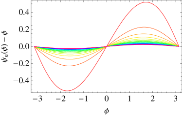
Figure 4: (Color online) Difference between the generalized angle coordinate $\psi_{n}(\phi)$ and $\phi$, here computed for $\sigma=0.44l$, $n_{0}=0$, and $n=1,\dots,20$. Larger differences occur at smaller $n$, where the effect of the external field is most noticeable.

Let us consider a closed Galton board of length $L=Nl$ ($2N+1$ disks) , with reflecting boundaries at $x=0$ and $x=L$. This is an equilibrium system. More precisely the invariant density associated to each disk is uniform, as verified in Fig. 5. The distinctive feature however is that the time scale changes with the disk index $n$, $\tau(n)\sim 1/v_{n}$. Thus particles move faster with increasing $n$, but correspondingly they make more collisions so that their distribution is uniform in time.

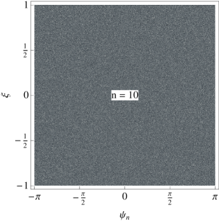
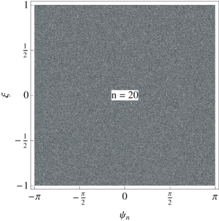
Figure 5: Invariant density associated to a closed Galton board of size $L=10l$, with reflection at the boundaries $x=0$ and $x=10l$, and energy $E=l/2$. This is an equilibrium system as reflected by the uniformity of the phase portraits.

From the average count of collision events of disk $n$, we obtain the collision frequency, which, when multiplied by the local time scale (this amounts to dividing it by the velocity $v_{n}$ evaluated at the center of cell $n$) yields the average density $P_{n}\sim\mathcal{P}(X_{n}=(n-1)l/2)$. This quantity, shown in Fig. 6, is indeed found to be almost constant, thus confirming our reasoning.

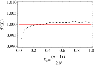
Figure 6: Equilibrium stationary density of the closed Galton board obtained for a channel of length $L=1$, with $2N+1$ disks, $N=25$. The solid line is the constant equilibrium density $\mathcal{P}(X)=1$.

II.5 Non-Equilibrium Galton Board

A non-equilibrium stationary state of the Galton board can be achieved much in the same way as with the open Lorentz gas studied in BGGi , by assuming that a flux of trajectories is continuously flowing through the boundaries which are let in contact with stochastic particle reservoirs at $x=0$ and $x=L$.

$$\rho(\Gamma,t)\Big{|}_{x=0,L}=\rho_{\pm}.$$ (37)

In analogy to the field free case, the invariant solution of the Liouville equation compatible with the boundary conditions (37) is given, for almost every phase point $\Gamma$, by

$$\rho(\Gamma) = \rho_{-}+\frac{\rho_{+}-\rho_{-}}{\sqrt{2(E+L)}-\sqrt{2E}}$$

$$\times\left[v(\Gamma)-\sqrt{2E}+\int_{0}^{-T(\Gamma)}dt\dot{v}(\Phi^{t}\Gamma)\right]\,.$$

Here $\rho(\Gamma)$ is written in terms of the change in velocity amplitude, given by $v(\Gamma)=\sqrt{2[E+x(\Gamma)]}$ at the corresponding horizontal position $x(\Gamma)$. Thus $\dot{v}(\Gamma)=[\dot{x}(\Gamma)]/v(\Gamma)$ and, provided the change in velocity between successive collisions is small, we can write $\int_{0}^{\tau}\dot{v}(\Phi^{t}\Gamma)dt\simeq[x(\Phi^{\tau}\Gamma)-x(\Gamma)]/v(\Gamma)$. Hence, denoting by $\tau_{k}$ the time separating the $(k-1)$th and $k$th collisions and by $t_{k}=\sum_{j=1}^{k}\tau_{k}$ the time elapsed after $k$ collisions, we have

$$\rho(\Gamma) \simeq \rho_{-}+\frac{\rho_{+}-\rho_{-}}{\sqrt{2(E+L)}-\sqrt{2E}}\Bigg{[}v(\Gamma)-\sqrt{2E}$$ (39)

$$+\sum_{k=1}^{K(\Gamma)}\frac{x(\Phi^{-t_{k}}\Gamma)-x(\Phi^{-t_{k-1}}\Gamma)}{v(\Phi^{-t_{k}}\Gamma)}\Bigg{]}\,.$$

This approximation becomes exact when the number of cells in the system is let to infinity, in which case $K(\Gamma)$, the number of collisions for the trajectory to reach the boundaries becomes infinite. Therefore the invariant state is

$$\rho(\Gamma) = \rho_{-}+\frac{\rho_{+}-\rho_{-}}{\sqrt{2(E+L)}-\sqrt{2E}}\Bigg{[}v(\Gamma)-\sqrt{2E}$$ (40)

$$+\sum_{k=1}^{\infty}\frac{x(\Phi^{-t_{k}}\Gamma)-x(\Phi^{-t_{k-1}}\Gamma)}{v(\Phi^{-t_{k}}\Gamma)}\Bigg{]}\,.$$

so that the fluctuating part of the invariant density becomes singular. This is analogous to the field free case discussed in BGGi .

We compute this quantity numerically from the statistics of the Birkhoff map of the Galton board, using a cylindrical Galton board similar to that shown in Fig. 1, with external forcing of unit magnitude in the direction of the cylinder axis, letting the particles have energy $E=1/2$. The particles are thus injected at $x=0$ with unit velocity at random angles and subsequently absorbed upon their first passage to either $x=0$ or $x=L$.

The computation of the collision frequency at disk $n$, averaged over the phase-space coordinates yields the quantity $\mu_{n}$, Eq. (29), which, after dividing by the modulus of the velocity at that site, is converted to $P_{n}$, the stationary solution of the Fokker-Planck equation (12). Here, we have

$$\mathcal{P}(X_{n}) = \frac{1}{l}\int_{\mathbb{C}_{n}\}}d\Gamma\rho(\Gamma)\,,$$ (41)

$$= \mathcal{P}_{-}+(\mathcal{P}_{+}-\mathcal{P}_{-})\frac{\sqrt{(E+X_{n})}-\sqrt{E}}{\sqrt{(E+L)}-\sqrt{E}}\,.$$

The results of this computation are presented in Fig. 7, and compared to Eqs. (18) and (32). The agreement with both discrete and continuous solutions is excellent.

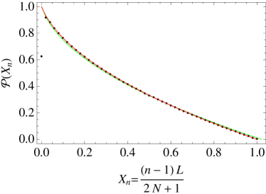
Figure 7: (Color online) Non-equilibrium stationary density of the Galton board obtained for a channel of length $L=1$, with $51$ disks ($N=25$). Two solid lines are shown which are barely distinguishable, corresponding to Eqs. (18) (Red) and (32) (Green) with $E=l/2$ and thus $n_{0}=0$.

The histograms displayed in Fig. 8 show the fluctuating part of the invariant phase-space density computed in terms of the Birkhoff coordinates $(\psi_{n},\xi)$, Eq. (36). The fractality of these graphs is much like that of the graphs of the open Lorentz gas, see BGGi . The differences are indeed too tenuous to tell. As with the closed Galton board though, the distinctive feature is that the collision rates increase with the cell index with the amplitude of the velocity.

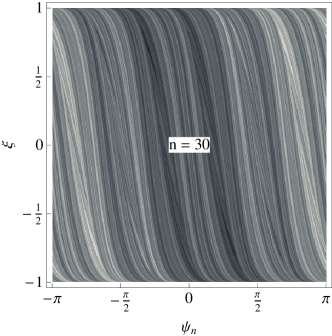
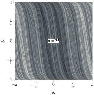
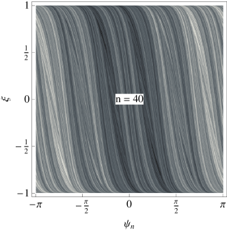
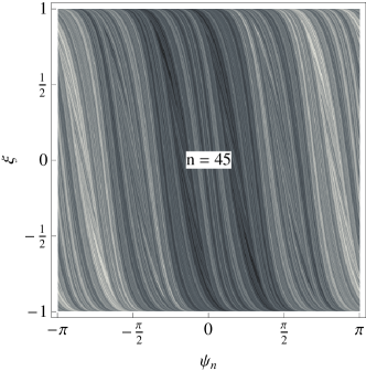
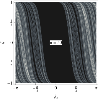
Figure 8: Non-equilibrium phase-space densities of the open Galton channel with a geometry similar to that shown in Fig. 1, with absorbing boundaries at $x=0$ and $x=1$, and stochastic injection of particles at $x=0$ only. Disk $50$ is the one before last. Black areas correspond to absorption at the nearby boundary. The color white is associated to injection from the left boundary. Thus hues of gray correspond to phase-space regions with mixtures of phase-space points which are mapped backward to the left and right borders. The corresponding overall densities are shown in Fig. 7.

To further analyze the fractality of the stationary state of the non-equilibrium Galton board and its relation to the phenomenological entropy production, Eq. (20), we introduce in the next section an analytically tractable model, which generalizes the multi-baker map associated to a field-free symmetric diffusion process, so as to account for the acceleration of tracer particles under the action of the external forcing.

III Forced multi-baker map

A time-reversible volume-preserving deterministic process can be associated to Eq. (25) in the form of a multi-baker map with energy, defined on the phase space ${(n,[0,l_{n}]\times[0,l_{n}])}_{n\in\mathbb{Z}}$, where each unit cell has area $l_{n}^{2}\equiv a_{n}l^{2}$, $a_{n}=\sqrt{}[1+(2n)/(2n_{0}+1)]$, and the dynamics is defined according to

$$B:\,(n,x,y)\mapsto\left\{\begin{array}[]{l@{\quad}l}\left(n-1,\frac{l_{n-1}}{l_{n}}\frac{x}{s_{n}^{-}},\frac{l_{n-1}}{l_{n}}s_{n-1}^{+}y\right)\,,&0\leq x\leq l_{n}s_{n}^{-},\\ \left(n,\frac{x-s_{n}^{-}l_{n}}{s_{n}^{0}},s_{n}^{+}l_{n}+s_{n}^{0}y\right)\,,&l_{n}s_{n}^{-}\leq x\leq l_{n}(1-s_{n}^{+})\,,\\ \left(n+1,\frac{l_{n+1}}{l_{n}}\frac{x-s_{n}^{-}l_{n}-s_{n}^{0}l_{n}}{s_{n}^{+}},\frac{l_{n+1}}{l_{n}}(s_{n+1}^{+}l_{n}+s_{n+1}^{0}l_{n}+s_{n+1}^{-}y)\right)\,,&l_{n}(1-s_{n}^{+})\leq x\leq l_{n}.\end{array}\right.$$ (42)

This map has two important properties. First, the areas of the unit cells are chosen to vary with the amplitude of the velocity, which ensures that the Jacobian of $B$, $\frac{a_{n-1}s_{n-1}^{+}}{a_{n}s_{n}^{-}}$ or $\frac{a_{n+1}s_{n+1}^{-}}{a_{n}s_{n}^{+}}$, is unity. Second, $B$ is time-reversal symmetric under the operator $S:\,(n,x,y)\to(n,l_{n}-y,l_{n}-x)$, i.e. $S\circ B=B^{-1}\circ S$, as is easily checked.

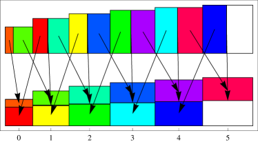
Figure 9: (Color online) Forced mutli-baker map (42). The cells have areas $a_{n}l^{2}$, with coordinates $(x,y)$, and labeled by a positive integer $n$ ($n_{0}=0$ here) . The map divides each cell into three vertical rectangles. The left rectangle is mapped to the bottom horizontal rectangle in the left neighboring cell. Likewise the right rectangle is mapped to the top horizontal rectangle in the right neighboring cell. The middle vertical rectangle is mapped to the middle horizontal rectangle in the same cell, but are so tiny they are barely visible already for $n=1$.

Multi-baker maps with energy have been considered earlier TG99 ; TG00 . The novelty here is to introduce $n$-dependent rates $s_{n}^{\pm}$ and $s_{n}^{0}$, Eq. (28). We will assume $D_{0}=1/2$ in the sequel, so that, provided $n_{0}+n\gg 1/2$, we can write

$$s_{n}^{\pm}=\frac{1}{2}\pm\frac{1}{4}\frac{1}{2(n_{0}+n)+1}-\frac{1}{16}\frac{1}{[2(n_{0}+n)+1]^{2}}+\dots$$ (43)

Thus $s_{n}^{0}=1-s_{n}^{+}-s_{n}^{-}$ is approximated by

$$s_{n}^{0}=\frac{1}{8}\frac{1}{[2(n_{0}+n)+1]^{2}}+\dots$$ (44)

which is vanishingly small. Therefore, when $n+n_{0}$ is large, the dynamics of $B$ reduces to that of the usual multi-baker map, at the exception of the energy dependence which fixes the local time scales.

III.1 Statistical ensembles

An initial density of points $\Gamma=(n,x,y)$, $\rho(\Gamma,0)$, evolves under repeated iterations of $B$ according to the action of the Frobenius-Perron operator, which, since $B$ preserves phase-space volumes, is simply given by $\rho(\Gamma,k+1)=\rho(B^{-1}\Gamma,k)$. In order to characterize the stationary density, $\rho(\Gamma)=\lim_{k\to\infty}\rho(\Gamma,k)$, we consider the cumulative function $\mu_{n}(x,y,k)=\int_{0}^{x}dx^{\prime}\int_{0}^{y}dy^{\prime}\rho(n,x^{\prime},y^{\prime},k)$. Notice that $\rho$ here refers to the statistics of the return map and therefore differs from the density $\rho$ associated to the Galton board, Eq. (40), by a factor proportional to the local time scale.

The identification of this function proceeds along the lines of Refs. TG95 ; TGD98 ; GD99 . Under the assumption that the $x$ dependence of the initial density is trivial, we can write $\mu_{n}(x,y,k)=x/\l_{n}\mu_{n}(l_{n},y,k)$. Letting $0\leq y\leq 1$, it is then easy to verify that $\mu_{n}(l_{n},y\,l_{n},k)$ obeys the functional equation

$$\mu_{n}(l_{n},y\,l_{n},k+1)=\left\{\begin{array}[]{l@{\quad}l}s_{n+1}^{-}\mu_{n+1}\left(l_{n+1},\frac{y}{s_{n}^{+}}l_{n+1},k\right)\,,&0\leq y\leq s_{n}^{+},\\ s_{n+1}^{-}\mu_{n+1}(l_{n+1},l_{n+1},k)+s_{n}^{0}\mu_{n}\left(l_{n},\frac{y-s_{n}^{+}}{s_{n}^{0}}l_{n},k\right)\,,&s_{n}^{+}\leq y\leq 1-s_{n}^{-},\\ s_{n+1}^{-}\mu_{n+1}(l_{n+1},l_{n+1},k)+s_{n}^{0}\mu_{n}(l_{n},l_{n},k)&\\ \quad+s_{n-1}^{+}\mu_{n-1}\left(l_{n-1},\frac{y-s_{n}^{+}-s_{n}^{0}}{s_{n}^{-}}l_{n-1},k\right)\,,&(1-s_{n}^{-})\leq y\leq 1.\end{array}\right.$$ (45)

In particular, letting $y=l_{n}$, we recover

$$\mu_{n}(l_{n},l_{n},k+1)=s_{n+1}^{-}\mu_{n+1}(l_{n+1},l_{n+1},k)$$

$$+s_{n}^{0}\mu_{n}(l_{n},l_{n},k)+s_{n-1}^{+}\mu_{n-1}(l_{n-1},l_{n-1},k)\,,$$

which is identical to Eq. (25) with $\mu_{n}(k)\equiv\mu_{n}(l_{n},l_{n},k)$. Let $\mu_{n}$ denote the steady state of this equation, $\mu_{n}=\lim_{k\to\infty}\mu_{n}(l_{n},l_{n},k)$.

The steady state of Eq. (45) can be written under the form, $0\leq x,y\leq 1$,

$$\mu_{n}(x\,l_{n},y\,l_{n}) \equiv \lim_{k\to\infty}\mu_{n}(x\,l_{n},y\,l_{n},k)\,,$$ (47)

$$= x\,y\,\mu_{n}+2x\,(s_{n+1}^{-}\mu_{n+1}-s_{n}^{+}\mu_{n})F_{n}(y)\,,$$

$$\equiv x\,y\,\mu_{n}+\alpha\,x\,F_{n}(y)\,,$$

where we introduced the generalized Takagi functions $F_{n}$, with a prefactor, $\alpha=2\big{(}s_{n+1}^{-}\mu_{n+1}-s_{n}^{+}\mu_{n}\big{)}$, which, as in Eqs. (II.2)-(32) is easily seen to be independent of $n$:

$$2\big{(}s_{n+1}^{-}\mu_{n+1}-s_{n}^{+}\mu_{n}\big{)} = \sqrt{\frac{2(n_{0}+n+1)}{2n_{0}+1}}(P_{n+1}-P_{n}),\,$$ (48)

$$= \sqrt{\frac{2}{2n_{0}+1}}\frac{P_{+}-P_{-}}{H_{N+n_{0}}^{1/2}-H_{n_{0}}^{1/2}}\,,$$

$$\to \frac{l}{2\sqrt{E}}\frac{P_{+}-P_{-}}{\sqrt{E+L}-\sqrt{E}}\,,$$

where the limit holds when $l\to 0$. Notice that the prefactor is proportional to $l$. Thus $\alpha$ is a small parameter in that limit.

Substituting Eq. (47) into Eq. (45), the generalized Takagi function $F$ is found to satisfy the functional equation

$$F_{n}(y)=$$ (53)

$$\left\{\begin{array}[]{l@{\quad}c}\frac{y}{2s_{n}^{+}}+s_{n+1}^{-}F_{n+1}\left(\frac{y}{s_{n}^{+}}\right)\,,&0\leq y<s_{n}^{+},\\ \frac{1}{2}+s_{n}^{0}F_{n}\left(\frac{y-s_{n}^{+}}{s_{n}^{0}}\right)\,,&s_{n}^{+}\leq y<1-s_{n}^{-},\\ \frac{1-y}{2s_{n}^{-}}+s_{n-1}^{+}F_{n-1}\left(\frac{y-s_{n}^{+}-s_{n}^{0}}{s_{n}^{-}}\right)\,,&1-s_{n}^{-}<y\leq 1.\end{array}\right.$$

The boundary conditions are such that the density is uniform at $n=0,N+1$, implying $F_{0}(y)=F_{N+1}(y)=0$. Notice that this function reduces to the Takagi function in the limit $n,N\to\infty$, $n\ll N$. Indeed $s_{\infty}^{-},s_{\infty}^{+}=1/2$, $s_{\infty}^{0}=0$. Therefore Eq. (47) is similar to the corresponding expression obtained for the multi-baker map, see BGGi .

III.1.1 Generalized Takagi functions

For the sake of plotting $F_{n}(y)$, it is convenient to consider the graph of $F_{n}(y)$ vs. $y$ as parameterized by a real variable, $0\leq x\leq 1$, defined so that

$$y_{n}(x)=$$ (58)

$$\left\{\begin{array}[]{l@{\quad}c}s_{n}^{+}y_{n+1}(3x)\,,&0\leq x<1/3,\\ s_{n}^{+}+s_{n}^{0}y_{n}(3x-1)\,,&1/3\leq x<2/3,\\ s_{n}^{+}+s_{n}^{0}+s_{n}^{-}y_{n-1}(3x-2)\,,&2/3\leq x<1,\end{array}\right.$$

and

$$F_{n}(x)=$$ (63)

$$\left\{\begin{array}[]{l@{\quad}c}\frac{y_{n}(x)}{2s_{n}^{+}}+s_{n+1}^{-}F_{n+1}(3x)\,,&0\leq x<1/3,\\ \frac{1}{2}+s_{n}^{0}F_{n}(3x-1)\,,&{1}/{3}\leq y<{2}/{3},\\ \frac{1-y_{n}(x)}{2s_{n}^{-}}+s_{n-1}^{+}F_{n-1}(3x-2)\,,&{2}/{3}\leq y<1.\end{array}\right.$$

The boundary conditions are taken so that $y_{n}(x)=y_{1}(x)$, $n<1$, and $y_{n}(x)=y_{N}(x)$, $n>N$. As above, $F_{n}(x)=0$, $n<1$ or $n>N$.

Starting from the end points $y(n,0)=0$, $y(n,1)=1$ and $F_{n}(0)=F_{n}(1)=0$, $1\leq n\leq N$, we successively compute $y_{n}(x_{k})$ and $F_{n}(x_{k})$, $1\leq n\leq N$ at points $x_{k}=\sum_{j=1}^{k}3^{-j}\omega_{j}$, where, for every $k\geq 1$, there are $3^{k}$ different sequences $\{\omega_{1},\dots,\omega_{k}\}$, $\omega_{j}\in\{0,1,2\}$, $1\leq j\leq k$.

The graphs of $F_{n}(x_{k})$ vs. $y_{n}(x_{k})$ are displayed in Fig. 10 for a chain of $N=100$ sites and $k=8$, and compared to the corresponding graphs of the incomplete Takagi functions TG95 , which can be obtained from Eq. (63) by setting $s_{n}^{+}=s_{n}^{-}\equiv 1/2$ and $s_{n}^{0}=0$,

$$y(x)=\left\{\begin{array}[]{l@{\quad}c}\frac{1}{2}y(3x)\,,&0\leq x<{1}/{3},\\ \frac{1}{2},&{1}/{3}\leq x<{2}/{3},\\ \frac{1}{2}+\frac{1}{2}y(3x-2)\,,&{2}/{3}\leq x<1,\end{array}\right.$$ (64)

and

$$T_{n}(x)=$$ (69)

$$\left\{\begin{array}[]{l@{\quad}c}y(x)+\frac{1}{2}T_{n+1}(3x)\,,&0\leq x<{1}/{3},\\ \frac{1}{2},&{1}/{3}\leq y<{2}/{3},\\ 1-y(x)+\frac{1}{2}T_{n-1}(3x-2)\,,&{2}/{3}\leq y<1.\end{array}\right.$$

In passing, we note that, on the one hand, Eq. (64) is a functional equation whose solution is the Cantor function. On the other hand, the tri-adic representation of the incomplete Takagi functions, Eq. (69), is many-to-one. Their graphs, $T_{n}(x)$ vs. $y(x)$, are nevertheless identical to those obtained using the usual representation of the incomplete Takagi functions.

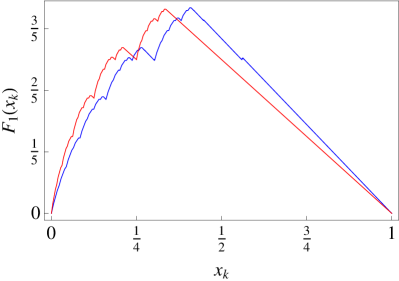
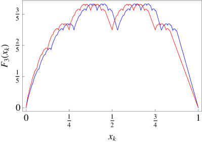
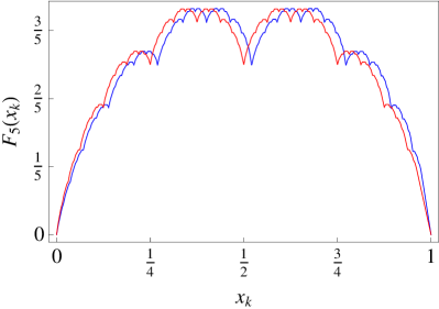
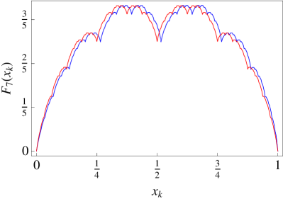
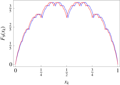
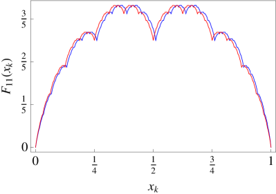
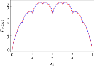
Figure 10: (Color online) Comparison between the graphs of $F_{n}(x_{k})$ vs. $y_{n}(x_{k})$ (Blue) and the corresponding incomplete Takagi functions $T_{n}(x_{k})$ (Red) . Each curve is computed at $3^{10}+1$ different points $x$, uniformly spread between $0$ and $1$. Only $2^{10}+1$ correspond to different points in the graphs of $T_{n}$.

III.1.2 Symbolic dynamics

By substituting the tri-adic expansion of $x$ in Eqs. (58)-(63), $x(\{\omega_{0},\dots,\omega_{k}\})=\sum_{j=0}^{k}\omega_{j}3^{-(j+1)}$, $\omega_{j}\in\{0,1,2\}$, we obtain the following symbolic representations of points $y$ in cell $n$,

$$y_{n}(\{\omega_{0},\dots,\omega_{k}\})=$$ (74)

$$\left\{\begin{array}[]{l@{\quad}c}s_{n}^{+}y_{n+1}(\{\omega_{1},\dots,\omega_{k}\})\,,&\omega_{0}=0,\\ s_{n}^{+}+s_{n}^{0}y_{n}(\{\omega_{1},\dots,\omega_{k}\})\,,&\omega_{0}=1,\\ s_{n}^{+}+s_{n}^{0}+s_{n}^{-}y_{n-1}(\{\omega_{1},\dots,\omega_{k}\})\,,&\omega_{0}=2.\end{array}\right.$$

Starting from

$$y_{n}(\{\omega_{0}\})=\left\{\begin{array}[]{l@{\quad}c}0,&\omega_{0}=0,\\ s_{n}^{+},&\omega_{0}=1,\\ s_{n}^{+}+s_{n}^{0},&\omega_{0}=2,\end{array}\right.$$ (75)

we can write

$$y_{n}(\{\omega_{0},\dots,\omega_{k}\})=$$

$$y_{n}(\{\omega_{0}\})+s_{n}^{1-\omega_{0}}y_{n+1-\omega_{0}}(\{\omega_{1},\dots,\omega_{k}\})\,,$$

$$= y_{n}(\{\omega_{0}\})+s_{n}^{1-\omega_{0}}y_{n+1-\omega_{0}}(\{\omega_{1}\})$$

$$+s_{n}^{1-\omega_{0}}s_{n+1-\omega_{0}}^{1-\omega_{1}}y_{n+2-\omega_{0}-\omega_{1}}(\{\omega_{2},\dots,\omega_{k}\})\,,$$

$$\vdots$$

$$= \sum_{i=0}^{k}\left[\prod_{j=0}^{i-1}s_{n+j-\omega_{0}-\dots-\omega_{j-1}}^{1-\omega_{j}}\right]y_{n+i-\omega_{0}-\dots-\omega_{i-1}}(\{\omega_{i}\})\,.$$

Substituting this symbolic dynamics into the expression of $F_{n}$, Eq. (53), we write

$$F_{n}(\{\omega_{0},\dots,\omega_{k}\})=\left\{\begin{array}[]{l@{\quad}c}\frac{1}{2}y_{n+1}(\{\omega_{1},\dots,\omega_{k}\})+s_{n+1}^{-}F_{n+1}(\{\omega_{1},\dots,\omega_{k}\})\,,&\omega_{0}=0,\\ 1/2+s_{n}^{0}F_{n}(\{\omega_{1},\dots,\omega_{k}\})\,,&\omega_{0}=1,\\ \frac{1}{2}(1-y_{n-1}(\{\omega_{1},\dots,\omega_{k}\}))+s_{n-1}^{+}F_{n-1}(\{\omega_{1},\dots,\omega_{k}\})\,,&\omega_{0}=2.\end{array}\right.$$ (77)

Let $\Delta y_{n}(\omega_{0},\dots,\omega_{k})$ denote the height of a horizontal cylinder set of the unit square, coded by the sequence $\{\omega_{0},\dots,\omega_{k}\}$. We have

$$\Delta y_{n}(\omega_{0},\dots,\omega_{k})\equiv$$

$$y_{n}(\{\omega_{0},\dots,\omega_{k}+1\})-y_{n}(\{\omega_{0},\dots,\omega_{k}\})\,,$$

where the notation $y_{n}(\{\omega_{0},\dots,\omega_{k}+1\})$ is literal whenever $\omega_{k}\neq 2$. Otherwise $y_{n}(\{\omega_{0},\dots,\omega_{k-1},2+1\})\equiv y_{n}(\{\omega_{0},\dots,\omega_{k-1}+1,0\})$ and we set $y_{n}(\{2,\dots,2,2+1\})\equiv 1$. We have the following identities

$$\left\{\begin{array}[]{lcl}\Delta y_{n}(0,\omega_{1},\dots,\omega_{k})&=&s_{n}^{+}\Delta y_{n+1}(\omega_{1},\dots,\omega_{k})\,,\\ \Delta y_{n}(1,\omega_{1},\dots,\omega_{k})&=&s_{n}^{0}\Delta y_{n}(\omega_{1},\dots,\omega_{k})\,,\\ \Delta y_{n}(2,\omega_{1},\dots,\omega_{k})&=&s_{n}^{-}\Delta y_{n-1}(\omega_{1},\dots,\omega_{k})\,.\end{array}\right.$$

Therefore

$$\Delta y_{n}(\omega_{0},\dots,\omega_{k})=\prod_{i=0}^{k}s_{n+i-\omega_{0}-\dots-\omega_{i-1}}^{1-\omega_{i}},$$ (79)

which is nothing but the probability associated to the trajectory starting at position $n$ and coded by the sequence $\{\omega_{0},\dots,\omega_{k}\}$.

Likewise, the measure of the cylinder set $\Delta y_{n}(\omega_{0},\dots,\omega_{k})$ is

$$\Delta\mu_{n}(\omega_{0},\dots,\omega_{k})\equiv\mu_{n}\big{(}y_{n}(\{\omega_{0},\dots,\omega_{k-1}+1\})\big{)}$$ (80)

$$-\mu_{n}\big{(}y_{n}(\{\omega_{0},\dots,\omega_{k-1}\})\big{)}\,,$$

$$= \mu_{n}\Delta y_{n}(\omega_{0},\dots,\omega_{k})+\alpha\Delta F_{n}(\omega_{0},\dots,\omega_{k})\,,$$

and we have the following set of identities for $\Delta F_{n}$:

$$\left\{\begin{array}[]{lcl}\Delta F_{n}(0,\omega_{1},\dots,\omega_{k})&=&\frac{1}{2}\Delta y_{n+1}(\omega_{1},\dots,\omega_{k})+s_{n+1}^{-}\Delta F{n+1}(\omega_{1},\dots,\omega_{k})\,,\\ \Delta F_{n}(1,\omega_{1},\dots,\omega_{k})&=&s_{n}^{0}\Delta F_{n}(\omega_{1},\dots,\omega_{k})\,,\\ \Delta F_{n}(2,\omega_{1},\dots,\omega_{k})&=&-\frac{1}{2}\Delta y_{n-1}(\omega_{1},\dots,\omega_{k})+s_{n-1}^{+}\Delta F_{n-1}(\omega_{1},\dots,\omega_{k})\,.\end{array}\right.$$ (81)

That is,

$$\Delta F_{n}(\omega_{0},\dots,\omega_{k})=\frac{1}{2}(1-\omega_{0})\Delta y_{n+1-\omega_{0}}(\omega_{1},\dots,\omega_{k})+s_{n+1-\omega_{0}}^{\omega_{0}-1}\Delta F_{n+1-\omega_{0}}(\omega_{1},\dots,\omega_{k})\,.$$ (82)

Notice that it is possible to solve this system recursively, starting from

$$\Delta F_{n}(\omega_{0})=\left\{\begin{array}[]{l@{\quad}c}1/2\,,&\omega_{0}=0\,,\\ 0\,,&\omega_{0}=1\,,\\ -1/2\,,&\omega_{0}=2\,.\end{array}\right.$$ (83)

We thus have a complete characterization of the non-equilibrium stationary state of $B$, Eq. (42), associated to flux boundary conditions.

III.2 Entropy and Entropy Production

We proceed along the lines of Gas97a ; GD99 to obtain expressions of the entropies and entropy production rates associated to coarse grained sets such as defined in Eq. (79). As described in BGGi , the idea is that, owing to the singularity of the invariant density, the entropy should be defined with respect to a grid of phase space, or partition, $\mathbb{G}=\{d\Gamma_{j}\}$, into small volume elements $d\Gamma_{j}$, and a time-dependent state $\mu_{n}(d\Gamma_{j},t)$. The entropy associated to cell $\mathbb{C}_{n}$, coarse grained with respect that grid, is defined according to

$$S_{\mathbb{G}}^{t}(\mathbb{C}_{n})=-\sum_{j}\mu_{n}(d\Gamma_{j},t)\left[\log\frac{\mu_{n}(d\Gamma_{j},t)}{d\Gamma_{j}}-1\right].$$ (84)

This entropy changes in a time interval $\tau$ according to

$$\Delta^{\tau}S^{t}(\mathbb{C}_{n}) = S_{\mathbb{G}}^{t}(\mathbb{C}_{n})-S_{\mathbb{G}}^{t-\tau}(\mathbb{C}_{n})\,,$$

$$= S_{\{d\Gamma_{j}\}}^{t}(\mathbb{C}_{n})-S_{\{\Phi^{\tau}d\Gamma_{j}\}}^{t}(\Phi^{\tau}\mathbb{C}_{n})\,,$$

where, in the second line, the collection of partition elements $\{d\Gamma_{j}\}$ was mapped to $\{\Phi^{\tau}d\Gamma_{j}\}$, which forms a partition $\Phi^{\tau}\mathbb{G}$ whose elements are typically stretched along the unstable foliations and folded along the stable foliations.

Following DGG02 , and in a way analogous to the phenomenological approach to entropy production deGMaz , the rate of entropy change can be further decomposed into entropy flux and production terms according to

$$\Delta^{\tau}S_{\mathbb{G}}^{t}(\mathbb{C}_{n})=\Delta_{\mathrm{e}}^{\tau}S_{\mathbb{G}}^{t}(\mathbb{C}_{n})+\Delta_{\mathrm{i}}^{\tau}S_{\mathbb{G}}^{t}(\mathbb{C}_{n})\,,$$ (86)

where the entropy flux is defined as the difference between the entropy that enters cell $\mathbb{C}_{n}$ and the entropy that exits that cell,

$$\Delta_{\mathrm{e}}^{\tau}S_{\mathbb{G}}^{t}(\mathbb{C}_{n})=S_{\{\Phi^{\tau}d\Gamma_{j}\}}^{t}(\mathbb{C}_{n})-S_{\{\Phi^{\tau}d\Gamma_{j}\}}^{t}(\Phi^{\tau}\mathbb{C}_{n})\,.$$ (87)

Collecting Eqs. (III.2)-(87), the entropy production rate at $\mathbb{C}_{n}$ measured with respect to the partition $\mathbb{G}$, is identified as

$$\Delta_{\mathrm{i}}^{\tau}S_{\mathbb{G}}^{t}(\mathbb{C}_{n})=S_{\{d\Gamma_{j}\}}^{t}(\mathbb{C}_{n})-S_{\{\Phi^{\tau}d\Gamma_{j}\}}^{t}(\mathbb{C}_{n})\,.$$ (88)

This formula is equally valid in the non-equilibrium stationary state.

Given a phase-space partition into the $3^{k}$ cylinder sets coded by the sequences $\underline{\omega}_{k}\equiv\{\omega_{0},\dots,\omega_{k-1}\}$, $\omega_{i}\in\{0,1,2\}$, as described in Sec. III.1, the $k$-entropy of the stationary state Eq. (47) relative to the volume measure of cell $n$ is defined by

$$S_{k}(\mathbb{C}_{n})=-\sum_{\underline{\omega}_{k}}\Delta\mu_{n}(\underline{\omega}_{k})\left[\log\frac{\Delta\mu_{n}(\underline{\omega}_{k})}{\Delta y_{n}(\underline{\omega}_{k})}-1\right]\,.$$ (89)

By summing over the first digit, it follows immediately from Eqs. (45) and (79) that the $k$-entropy verifies a recursion relation,

$$S_{k}(\mathbb{C}_{n}) = -s_{n+1}^{-}\rho_{n+1}\log\frac{s_{n+1}^{-}}{s_{n}^{+}}-s_{n-1}^{+}\rho_{n-1}\log\frac{s_{n-1}^{+}}{s_{n}^{-}}$$ (90)

$$+s_{n+1}^{-}S_{k-1}(\mathbb{C}_{n+1})+s_{n}^{0}S_{k-1}(\mathbb{C}_{n})$$

$$+s_{n-1}^{+}S_{k-1}(\mathbb{C}_{n-1})\,,$$

with the $0$-entropy given by

$$S_{0}(\mathbb{C}_{n})=-\mu_{n}\log\mu_{n}\,,$$ (91)

and boundary conditions

$$\left\{\begin{array}[]{lcl}S_{k}(\mathbb{C}_{0})&=&-\rho_{-}\log\rho_{-}\,,\\ S_{k}(\mathbb{C}_{N+1})&=&-\rho_{+}\log\rho_{+}\,.\end{array}\right.$$ (92)

The $k$-entropy can be computed based on the above recursion relation. However, in order to obtain the dependence of the entropy on the resolution parameter $k$, it is more useful to consider the expansion of Eq. (89) in powers of $\rho_{n}$. Let us denote by $\underline{\omega}_{k}$ the sequence $\{\omega_{0},\dots,\omega_{k-1}\}$

$$S_{k}(\mathbb{C}_{n}) = -\mu_{n}\sum_{\underline{\omega}_{k}}\Delta y_{n}(\underline{\omega}_{k})\left[1+\frac{\alpha}{\mu_{n}}\frac{\Delta F_{n}(\underline{\omega}_{k})}{\Delta y_{n}(\underline{\omega}_{k})}\right]\left\{\log\mu_{n}\left[1+\frac{\alpha}{\mu_{n}}\frac{\Delta F_{n}(\underline{\omega}_{k})}{l\Delta y_{n}(\underline{\omega}_{k})}\right]-1\right\}\,,$$ (93)

$$= -\mu_{n}(\log\mu_{n}-1)-\alpha(\log\mu_{n}-1)\sum_{\underline{\omega}_{k}}\Delta F_{n}(\underline{\omega}_{k})-\frac{\alpha^{2}}{2\mu_{n}}\sum_{\underline{\omega}_{k}}\frac{[\Delta F_{n}(\underline{\omega}_{k})]^{2}}{\Delta y_{n}(\underline{\omega}_{k})}+\mathcal{O}(\alpha)^{3}\,.$$

The second term on the RHS of this equation vanishes, since

$$\sum_{\underline{\omega}_{k}}\Delta F_{n}(\underline{\omega}_{k})=0.$$ (94)

As of the third term on the RHS of Eq. (93), proportional to $\alpha^{2}$, we have, using Eqs. (III.1.2) and (81),

$$\Delta^{2}_{n}(k) \equiv \sum_{\underline{\omega}_{k}}\frac{[\Delta F_{n}(\underline{\omega}_{k})]^{2}}{\Delta y_{n}(\underline{\omega}_{k})}\,,$$ (95)

$$= \frac{1}{4s_{n}^{+}}+\frac{1}{4s_{n}^{-}}+\frac{(s_{n+1}^{-})^{2}}{s_{n}^{+}}\Delta^{2}_{n+1}(k-1)+s_{n}^{0}\Delta^{2}_{n}(k-1)+\frac{(s_{n-1}^{+})^{2}}{s_{n}^{-}}\Delta^{2}_{n-1}(k-1)$$

$$= \frac{1}{4s_{n}^{+}}+\frac{1}{4s_{n}^{-}}+\sum_{\eta=0}^{2}\frac{(s^{\eta-1}_{n+1-\eta})^{2}}{s^{1-\eta}_{n}}\Delta^{2}_{n+1-\eta}(k-1),$$

$$= \sum_{i=0}^{k-1}\sum_{\eta_{1},\dots,\eta_{i-1}}\left[\prod_{j=1}^{i}\frac{(s^{\eta_{j}-1}_{n+j-\eta_{1}-\dots-\eta_{j}})^{2}}{s^{1-\eta_{j}}_{n+j-1-\eta_{1}-\dots-\eta_{j-1}}}\right]\left(\frac{1}{4s_{n+i-\eta_{1}-\dots-\eta_{i}}^{+}}+\frac{1}{4s_{n+i-\eta_{1}-\dots-\eta_{i}}^{-}}\right)\,.$$ (96)

Substituting the expressions of the probability transitions from Eqs. (43)-(44), Eq. (96) is found to be

$$\Delta^{2}_{n}(k) = \sum_{\underline{\omega}_{k}}\frac{[\Delta F_{n}(\underline{\omega}_{k})]^{2}}{\Delta y_{n}(\underline{\omega}_{k})}\,,$$ (97)

$$= k+\frac{12k^{2}-9k}{32(n+n_{0})^{2}}+\mathcal{O}(n+n_{0})^{-4}\,.$$

The first term on the RHS of this expression, which is the only term that survives in the continuum limit where $n+n_{0}\gg 1$, is responsible for the linear decay of the $k$-entropy,

$$S_{k}(\mathbb{C}_{n})\simeq-\mu_{n}(\log\mu_{n}-1)-\frac{\alpha^{2}}{2\mu_{n}}k\,.$$ (98)

Indeed if follows from Eq. (88) that the $k$-entropy production rate is here

$$\Delta_{\mathrm{i}}^{\tau}S_{k}(\mathbb{C}_{n}) = \frac{1}{\tau}\left[S_{k}(\mathbb{C}_{n})-S_{k+1}(\mathbb{C}_{n})\right],$$

$$= \frac{\alpha^{2}}{2\tau\mu_{n}}\,.$$

Using Eqs. (10), (29) and (48), it is readily checked that this expression yields the phenomenological entropy production rate, Eq. (20), $\Delta_{\mathrm{i}}^{\tau}S_{k}(\mathbb{C}_{n})\stackrel{{\scriptstyle\tau,l\to 0}}{{\to}}d_{\mathrm{i}}S(X=nl)/dt$.

IV Conclusions

In this paper, we have considered the influence of an external field on a class of time-reversible deterministic volume-preserving models of diffusive systems known as Galton boards or, equivalently, forced periodic two-dimensional Lorentz gases.

Though the particles are accelerated as they move along the direction of the external field, in the absence of a dissipative mechanism, the motion is recurrent, which is to say that tracer particles keep coming back to the region of near zero velocity. In other words, particles do not drift in the direction of the external field. Rather, forced periodic Lorentz gases remain purely diffusive in two dimensions, albeit with a velocity-dependent diffusion coefficient. Consequently, the scaling laws relating time and displacement are different from that of a homogeneously diffusive system. The macroscopic description through a Fokker Planck equation is however unchanged since the mobility coefficient vanishes identically in dimension 2.

It will be interesting to investigate the behavior of three-dimensional periodic Lorentz gases in a uniform external field. As our analysis showed, the mobility does not vanish in dimension three, so that the Fokker-Planck equation retains a drift term. Being inversely proportional to the tracers’ velocity amplitudes, this drift decreases with increasing kinetic energy. A cross-over is thus expected between biased and diffusive motions.

As far as their statistical properties are concerned, Galton boards are essentially identical to the field-free periodic two-dimensional Lorentz gases. A closed system with reflecting boundaries relaxes to an equilibrium state with a uniform invariant measure. This is to say that tracers spend equal amounts of time in all parts of the system. Open systems with absorbing boundaries yield non-equilibrium states. Given constant rates of tracer injection at the borders, the system reaches a non-equilibrium stationary state which is characterized by a fractal invariant measure.

The fractality of the invariant measure associated to the non-equilibrium state of such a system was established analytically for a multi-baker map describing the motion of random walkers accelerated by a uniform external field. The computation of the coarse grained entropies associated to arbitrarily refined partitions yields expressions which depart from their local equilibrium expressions by a term which decreases linearly with the logarithm of the number of elements in the partition. This term is responsible for the positiveness of the entropy production rate, with a value consistent with the phenomenological expression of thermodynamics.

- (1) F. Galton, Natural inheritance (Macmillan, 1889).
- (2) M. Barile and E. W. Weisstein, Galton Board, From MathWorld–A Wolfram Web Resource. http://mathworld.wolfram.com/GaltonBoard.html
- (3) H.A. Lorentz, The motion of electrons in metallic bodies, Proc. R. Acad. Amsterdam 7 438, 585, 684 (1905).
- (4) H. van Beijeren, Transport properties of stochastic Lorentz models, Rev. Mod. Phys. 54 195 (1982).
- (5) C.P. Dettmann, The Lorentz gas as a paradigm for nonequilibrium stationary states, in: D. Szasz (Ed.) , Hard Ball Systems and Lorentz Gas, Encyclopaedia of Mathematical Sciences (Springer, Berlin, 2000).
- (6) S. Chapman and T.G. Cowling, The Mathematical Theory of Non-uniform Gases, 3rd Edition (Cambridge University Press, Cambridge, UK, 1970) (Chapter 10).
- (7) E. H. Hauge, What can one learn from Lorentz models?, in: G. Kirczenow, J. Marro (Eds.), Transport Phenomena, (Springer, Berlin, 1974).
- (8) L. A. Bunimovich and Ya. G. Sinai, Markov Partitions for dispersed billiards, Commun. Math. Phys. 78 247 (1980); Statistical properties of lorentz gas with periodic configuration of scatterers, Commun. Math. Phys. 78 479 (1981).
- (9) W. G. Hoover, Molecular Dynamics, (Springer-Verlag, Heidelberg, 1986)
- (10) D. J. Evans and G. P. Morriss, Statistical Mechanics of Non-Equilibrium Liquids, 2nd edition (Cambridge University Press, Cambridge UK, 2008).
- (11) B. Moran and W. Hoover, Diffusion in a periodic Lorentz gas, J. Stat. Phys. 48 709 (1987).
- (12) N. I. Chernov, G. L. Eyink, J. L. Lebowitz, Ya. G. Sinai, Derivation of Ohm’s law in a deterministic mechanical model, Phys. Rev. Lett. 70 2209 (1993); Steady-state electrical conduction in the periodic Lorentz gas, Commun. Math. Phys. bf 154 569 (1993).
- (13) P. Drude, Zur Elektronentheorie der Metalle Annalen der Physik, 1 566 (1900); 3 369 (1900).
- (14) N. W. Ashcroft and N. D. Mermin, Solid state phyics, (Brooks/Cole, 1976).
- (15) F. Barra, P. Gaspard and T. Gilbert, Fractality of the non-equilibrium stationary states of open volume-preserving systems: I. Tagged particle diffusion, preprint (2008).
- (16) S. Tasaki and P. Gaspard, Thermodynamic behavior of an area-preserving multibaker map with energy, Theor. Chem. Acc. 102 385 (1999).
- (17) S. Tasaki and P. Gaspard, Entropy Production and Transports in a Conservative Multibaker Map with Energy, J. Stat. Phys. 101 125 (2000).
- (18) S. Tasaki and P. Gaspard, Fick’s law and fractality of nonequilibrium stationary states in a reversible multibaker map, J. Stat. Phys. 81 935 (1995).
- (19) J. Machta and R. Zwanzig Diffusion in a periodic Lorentz gas, Phys. Rev. Lett. 50 1959 (1983).
- (20) N. Chernov and D. Dolgopyat, Diffusive motion and recurrence on an idealized Galton board, Phys. Rev. Lett. 99 030601 (2007).
- (21) N. Chernov and D. Dolgopyat, Galton Board: limit theorems and recurrence, preprint (2007).
- (22) P. Gaspard, Chaos, scattering and statistical mechanics, (Cambridge University Press, Cambridge, 1998).
- (23) P. Gaspard, Chaos and hydrodynamics, Physica A 240 54 (1997).
- (24) J. L. Lebowitz, Stationary Nonequilibrium Gibbsian Ensembles, Phys. Rev. 114 1192 (1959).
- (25) J. A. McLennan, Statistical Mechanics of the Steady State, Phys. Rev. 115 1405 (1959).
- (26) P. Gaspard, Diffusion, effusion, and chaotic scattering: An exactly solvable Liouvillian dynamics, J. Stat. Phys. 68 673 (1992).
- (27) P. Gaspard, Entropy production in open volume-preserving systems, J. Stat. Phys. 88 1215 (1997).
- (28) G. de Rham, Sur un exemple de fonction continue sans dérivée, Enseign. Math. 3, 71 (1957); Sur quelques courbes définies par des équations fonctionnelles Rend. Sem. Mat. Torino 16, 101 (1957).
- (29) T. Takagi, A simple example of continuous function without derivative, Proc. Phy.-Math. Soc. Japan 1 176 (1903).
- (30) R. C. Tolman, The Principles of Statistical Mechanics, (Oxford, London, 1938); reprinted (Dover Publications, New York, 1979).
- (31) P. and T. Ehrenfest, The Conceptual Foundations of the Statistical Approach in Mechanics, (Cornell University Press, Ithaca, 1959); reprinted (Dover Publications, New York, 2002).
- (32) T. Gilbert and J. R. Dorfman, Entropy Production : From Open Volume Preserving to Dissipative Systems, J. Stat. Phys. 96 225 (1999).
- (33) Wikipedia contributors, Quartic equation, Wikipedia, The Free Encyclopedia, http://en.wikipedia.org/wiki/Quartic_equation
- (34) P. Gaspard, G. Nicolis and J. R. Dorfman, Diffusive Lorentz gases and multibaker maps are compatible with irreversible dynamics, Physica A 323 294-322 (2003).
- (35) J. Sondow and E. W. Weisstein Harmonic Number, From MathWorld–A Wolfram Web Resource. http://mathworld.wolfram.com/HarmonicNumber.html
- (36) S. Koga, Unified treatment of Birkhoff coordinates in billiard systems of particles moving under an influence of a potential including particle-particle interaction, J. Phys. Soc. Japan 70 1260 (2001).
- (37) S. Tasaki, T. Gilbert and J. R. Dorfman, An Analytical Construction of the SRB Measures for Baker-type Maps, Chaos 8 424 (1998).
- (38) J. R. Dorfman, P. Gaspard and T. Gilbert, Entropy production of diffusion in spatially periodic deterministic systems, Phys. Rev. E 66 026110 (2002).
- (39) S. de Groot and P. Mazur, Non-equilibrium Thermodynamics, (North-Holland, Amsterdam, 1962); reprinted (Dover Publ. Co., New York, 1984).