Interplay of noise and coupling in heterogeneous ensembles of phase oscillators

Abstract

We study the effects of noise on the collective dynamics of an ensemble of coupled phase oscillators whose natural frequencies are all identical, but whose coupling strengths are not the same all over the ensemble. The intensity of noise can also be heterogeneous, representing diversity in the individual responses to external fluctuations. We show that the desynchronization transition induced by noise may be completely suppressed, even for arbitrarily large noise intensities, is the distribution of coupling strengths decays slowly enough for large couplings. Equivalently, if the response to noise of a sufficiently large fraction of the ensemble is weak enough, desynchronization cannot occur. The two effects combine with each other when the response to noise and the coupling strength of each oscillator are correlated. This combination is quantitatively characterized and illustrated with explicit examples.

The statistical description of a large physical system, formed by a multitude of interacting elements, is admittedly simpler if all the elements are mutually identical. In such a homogeneous ensemble, every element is representative of any other, which simplifies the calculation of average quantities and collective properties, both static and dynamic. Many applications require however the consideration of heterogeneous ensembles to account for various sources of diversity, from dispersion in the parameters that govern the individual dynamics of the elements and their interaction, to differences in the external influences, such as noise, that affect each element independently fromcells .

Kuramoto’s theory for the synchronization of coupled oscillators kura is an instance where heterogeneity plays a key role in the collective behaviour of a large ensemble. The synchronization transition, between states of incoherent and coherent dynamics, results from the competition of the strength of coupling and the dispersion in the natural frequencies of individual oscillators win . Further sources of heterogeneity are, for instance, the topology of connection patterns red1 ; red2 and diversity in the interaction laws between oscillator pairs fases .

In this paper, we study an extension of Kuramoto’s model, with two additional sources of diversity, which still admits a fully analytical treatment. Consider an ensemble of $N$ phase oscillators, each of them characterized by a phase $\phi_{i}\in[0,2\pi)$. The dynamics of phases is given by

$$\dot{\phi}_{i}=\omega_{i}+\frac{k_{i}}{N}\sum_{j=1}^{N}\sin(\phi_{j}-\phi_{i})+\xi_{i}(t),$$ (1)

$i=1,\dots,N$, where $\omega_{i}$ is the natural frequency of oscillator $i$, $k_{i}>0$ is the coupling strength for the same oscillator. In the standard Kuramoto’s model, all oscillators have identical coupling strengths, $k_{i}=K$ for all $i$. The non-correlated Gaussian noises $\xi_{i}(t)$ have zero mean, and $\langle\xi_{i}(t)\xi_{j}(t^{\prime})\rangle=2s_{i}\delta_{ij}\delta(t-t^{\prime})$. Note that here we admit that the intensity of noise, $s_{i}>0$, may be different for each oscillator, standing for diversity in the response to external fluctuations.

As in the standard model kura ; nos , equation (1) can be recast as

$$\dot{\phi}_{i}=\omega_{i}+k_{i}\sigma\sin(\Phi-\phi_{i})+\xi_{i}(t),$$ (2)

with

$$\sigma\exp({\rm i}\Phi)=\frac{1}{N}\sum_{j=1}^{N}\exp({\rm i}\phi_{j}).$$ (3)

The non-negative number $\sigma$ is the Kuramoto order parameter, which characterizes the synchronization transition: $\sigma=0$ represents an incoherent state with uniform distribution of phases, while $\sigma>0$ reveals a certain degree of organization in the phases, that we associate with synchronization.

In previous work pais1 ; pais2 , we have studied the extended model (2) in the absence of noise, $s_{i}\equiv 0$ for all $i$. Heterogeneous coupling strengths make it possible that an oscillator whose natural frequency is far from the synchronization frequency becomes nevertheless entrained in synchronized behaviour if its coupling strength is large enough. Synchronization is thus enhanced. If, on the other hand, oscillators close to the synchronization frequency have systematically low coupling strengths, synchronization may be completely suppressed.

Here, we focus our attention on the case where the natural frequencies of all oscillators are identical, $\omega_{i}=\omega$ for all $i$. The transformation $\phi_{i}\to\phi_{i}+\omega t$ for all $i$ makes it possible to take, without generality loss, $\omega\equiv 0$. Now, moreover, external noise is present: $s_{i}\neq 0$. Heterogeneity in the intrinsic dynamics of the oscillators, given by their natural frequencies, is thus replaced by fluctuations in the form of additive noise.

In order to provide a statistical description of our system in the limit $N\to\infty$, we introduce $n(k,s;\phi,t)$, the density of oscillators with coupling strength $k$ and noise intensity $s$ which, at time $t$, have phase $\phi$. Standard results from the theory of stochastic processes stoch establish that, if equation (1) governs the dynamics of phases, the density $n(k,s;\phi,t)$ satisfies the Fokker-Planck equation

$$\partial_{t}n=s\partial^{2}_{\phi}n+k\sigma\partial_{\phi}[n\sin(\phi-\Phi)].$$ (4)

The stationary solution to this equation, obtained from $\partial_{t}n\equiv 0$, reads

$$n(k,s;\phi)=\frac{1}{2\pi I_{0}(k\sigma/s)}\exp\left[\frac{k\sigma}{s}\cos(\phi-\Phi)\right],$$ (5)

where $I_{\nu}(x)$ is the order-$\nu$ modified Bessel function of the first kind abramo . This solution, which is expected to represent the long-time, equilibrium distribution of phases, remains however a formal expression, since both $\sigma$ and $\Phi$ are still unknown.

To obtain self-consistent values for $\sigma$ and $\Phi$, we transform equation (3) into its continuous version by using the oscillator density $n$. To do this, we assume that the interaction strengths $k_{i}$ and the noise intensities $s_{i}$ are assigned over the ensemble following a prescribed distribution $W(k,s)$. The normalization of this distribution requires

$$\int_{0}^{\infty}dk\int_{0}^{\infty}ds\,W(k,s)=1.$$ (6)

Note that, since both the interaction strength and the noise intensity of a given oscillator measure its response to extrinsic actions –respectively, the rest of the ensemble and fluctuations– it is not unlikely that they are correlated attributes, so that $W(k,s)$ cannot generally be factorized. The sum over oscillators in equation (3) becomes thus a multiple integral over $k$, $s$, and the phase $\phi$. Using the equilibrium density of equation (5), we get

$$\sigma= \displaystyle{\int_{0}^{2\pi}d\phi\int_{0}^{\infty}dk\int_{0}^{\infty}ds\,\frac{W(k,s)}{2\pi I_{0}(k\sigma/s)}}$$ (7)

$$\times\exp\left(\displaystyle{\frac{k\sigma}{s}}\cos\phi\right)\exp\left({\rm i}\phi\right).$$

Due to the fact that the integrand is $2\pi$-periodic in $\phi$ and that the integral over the phase runs over a whole period, the value of the collective phase $\Phi$ is arbitrary; we have chosen $\Phi=0$. Performing the integral over $\phi$, we find

$$\sigma=\int_{0}^{\infty}dk\int_{0}^{\infty}ds\,W(k,s)\frac{I_{1}(k\sigma/s)}{I_{0}(k\sigma/s)}.$$ (8)

This implicit equation for $\sigma$ is our main result. It determines the order parameter in terms of the density of interaction strengths and noise intensities, $W(k,s)$. It always has a trivial solution $\sigma=0$ which, according to equation (5), corresponds to a uniform phase distribution $n(k,s;\phi)=(2\pi)^{-1}$. Synchronized states are those where, on the contrary, $\sigma\neq 0$.

For homogeneous interaction strengths and noise intensities, $k_{i}=K$ and $s_{i}=S$ for all $i$, we have $W(k,s)=\delta(k-K)\delta(s-S)$. Equation (8) reduces to

$$\sigma=I_{1}(K\sigma/S)/I_{0}(K\sigma/S),$$ (9)

a limit that has already been analyzed in the literature fromcells . For large intensity noises, the only solution is $\sigma=0$, and the oscillator ensemble is unsynchronized. On the other hand, a positive solution exists if $S$ is sufficiently small. This solution appears through a pitchfork bifurcation at the critical noise intensity $S_{c}=K/2$. It approaches $\sigma=1$, corresponding to complete synchronization, as $S\to 0$.

To study how this scenario changes when interaction strengths and noise intensities are not the same all over the ensemble, we first analyze the behaviour of the right-hand side of equation (8) –which, for conciseness, we call $J(\sigma)$– as a function of $\sigma$. We assume that the distribution $W(k,s)$, which must satisfy the normalization (6), is regular enough as to warrant the conclusions drawn in the following. Since $I_{0}(0)=1$ and $I_{1}(0)=0$, $J(\sigma)$ vanishes as $\sigma\to 0$. The ratio $I_{1}(x)/I_{0}(x)$, in turn, tends to one as $x\to\infty$. Therefore, by virtue of equation (6), $J(\sigma)$ also approaches one as $\sigma\to\infty$. Assuming that $J(\sigma)$ varies monotonically from zero to one as $\sigma$ grows from zero to infinity, equation (8) will have a single solution at $\sigma=0$ if the slope of $J(\sigma)$ at that point is lower than one. On the other hand, a non-trivial solution will exist if the slope is greater than one. Straightforward calculation of the derivatives of the Bessel functions at zero shows that this condition, which fixes the threshold for synchronization, is equivalent to

$$1=\int_{0}^{\infty}dk\int_{0}^{\infty}ds\,\frac{k}{2s}W(k,s).$$ (10)

This equation must be interpreted as a condition to be fulfilled by the parameters that define the distribution $W(k,s)$. In parameter space, it determines the boundary between regions of synchronized and unsynchronized dynamics, namely, the desynchronization boundary.

To appraise how equation (10) works, let us analyze two extreme situations. In the first situation, the coupling strength and the noise intensity of each oscillator are fully uncorrelated attributes, so that their distribution can be factorized as $W(k,s)=W_{1}(k)W_{2}(s)$. Suppose also that $W_{2}(s)=\delta(s-S)$, so that the noise intensity is equal to $S$ all over the ensemble. In this case, equation (10) establishes that the critical noise intensity is

$$S_{c}=\frac{1}{2}\int_{0}^{\infty}dk\,kW_{1}(k).$$ (11)

From this result we draw our first important conclusion: in an ensemble with heterogeneous coupling, noise is able to suppress synchronization as long as the function $kW_{1}(k)$ is integrable over $(0,\infty)$. In other words, if the distribution of coupling strengths decays slowly enough for $k\to\infty$ –namely, as $W_{1}\sim k^{-p}$ with $1<p<2$– synchronized behaviour persists even for arbitrarily large external fluctuations.

For more general forms of $W_{2}(s)$, the factorization of $W(k,s)$ implies that the right-hand side of equation (10) is a product of two integrals, respectively over $k$ and $s$. The equation can hold only if the two integrals converge. In particular, the function $s^{-1}W_{2}(s)$ must be integrable over $(0,\infty)$. Now, therefore, fluctuations are able to suppress synchronized behaviour only if $W_{2}(s)$ vanishes for $s\to 0$. Specifically, if the fraction of the ensemble with noise intensities below a small threshold $\delta s$ is proportional to $\delta s$ (or larger), too many oscillators are subject to too weak noise, and fluctuations cannot inhibit synchronization.

At the opposite extreme, we examine the case where the correlation between coupling strength and noise intensity is so strong that one of the two attributes is a given function of the other. We take $s\equiv\zeta(k)$, so that $W(k,s)=W_{1}(k)\delta[s-\zeta(k)]$. Equation (10) becomes

$$1=\int_{0}^{\infty}dk\,\frac{k}{2\zeta(k)}W_{1}(k).$$ (12)

A necessary condition for this equation to hold is now that the function $kW_{1}(k)/\zeta(k)$ is integrable over $(0,\infty)$. In particular, the distribution of coupling strengths may decay as slowly as to make the product $kW_{1}(k)$ non-integrable. But if, at the same time, the intensity of noise grows sufficiently fast with the coupling strength, the desynchronization transition can still take place. As for the integrability condition at $k\to 0$, the integral may diverge if the noise intensity $\zeta(k)$ exhibits a sufficiently fast decay with the coupling strength.

Let us illustrate these conclusions with results for the order parameter $\sigma$ corresponding to some specific forms of the distribution of coupling strengths and noise intensities, chosen in such a way as to exemplify the different situations analyzed above. Generally, equation (8) must be solved by numerical means, as explicit expressions for the involved integrals are usually not known.

Consider first the case where the noise intensity $S$ is the same all over the ensemble. For the distribution of coupling strengths, we take

$$W_{1}(k)=(p-1)(1+k)^{-p}$$ (13)

with $p>1$, i.e. a power-law decaying function of $k$. Figure 1 shows the order parameter as a function of the noise intensity for several values of $p$. As expected, in all cases, the degree of synchronization decreases with noise. The critical noise intensity at which the order parameter vanishes, $S_{c}=[2(p-2)]^{-1}$, is well defined for $p>2$. Note also that the behaviour of $\sigma$ at the critical point varies with $p$. Approximating equation (8) for $\sigma\approx 0$, in fact, we find $\sigma\approx\alpha(S_{c}-S)^{1/(p-2)}$, with $\alpha$ a constant. For $1<p\leq 2$, the order parameter decays indefinitely, never reaching zero, as $S$ grows. The inset of Figure 1 shows, in gray, the zone of parameter space where synchronized dynamics occurs. This phase diagram suggests that the behaviour of the order parameter as a function of $p$, for fixed noise intensity, would be qualitatively the same as shown in the main plot as a function of $S$.

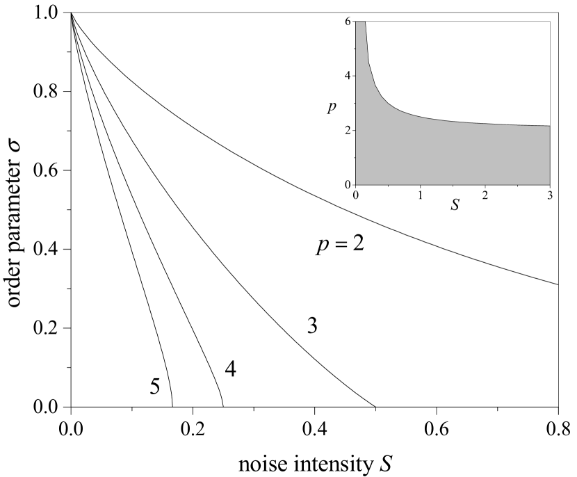
Figure 1: Kuramoto order parameter $\sigma$ as a function of the noise intensity $S$ in an ensemble of coupled oscillators with coupling strength distribution $W_{1}(k)=(p-1)(1+k)^{-p}$, for several values of $p$. The inset shows the synchronization region ($\sigma\neq 0$; shaded) in the parameter plane $(S,p)$.

Next, we consider that the noise intensity is heterogeneous, but still uncorrelated to the coupling strength. We take

$$W_{2}(s)=w_{0}s^{q}\exp[-(q+1)s/S],$$ (14)

where $w_{0}$ is a normalization constant. The exponent $q>-1$, controls the shape of the distribution at $s=0$. For $q>0$, the distribution vanishes at the origin and has a maximum at $s=Sq/(q+1)$. As $q\to\infty$, it approaches $W_{2}(s)=\delta(s-S)$, the case considered in the preceding paragraph. For $q=0$, the distribution is a purely decaying exponential, and for $q<0$ it diverges as $s$ approaches zero. As for the distribution of coupling strengths, we take the same as in equation (13) with $p=3$, namely, $W_{1}(k)=2(1+k)^{-3}$. In Figure 2, we plot the order parameter $\sigma$ as a function of the noise parameter $S$, for several values of the exponent $q$. The curve for $q\to\infty$ coincides with that of Figure 1 for $p=3$. The critical noise parameter at which $\sigma$ vanishes, $S_{c}$, shifts to higher values as $q$ decreases. Its analytical evaluation, in fact, shows that the desynchronization transition takes place at $S_{c}=(1+q)/2q$. As expected, $q=0$ is the largest value of $q$ for which noise is not able to suppress synchronization. For smaller exponents, the distribution of noise intensities does not vanish at $s=0$, and synchronized behaviour persists even for arbitrarily large values of $S$.

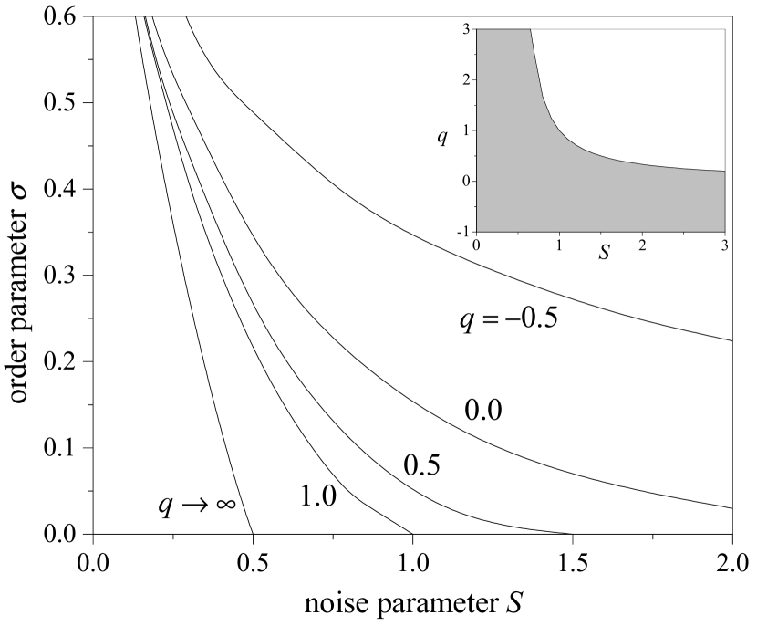
Figure 2: Kuramoto order parameter $\sigma$ as a function of the parameter $S$ in an ensemble of coupled oscillators with noise intensity distribution $W_{2}(s)\propto s^{q}\exp[-(q+1)s/S]$, for several values of $q$. The coupling strength distribution is as in fig. 1, with $p=3$. The inset shows the synchronization region ($\sigma\neq 0$; shaded) in the parameter plane $(S,q)$.

Finally, we study a case where there is correlation between the coupling strength and the noise intensity of each oscillator. However, instead of taking –as in the derivation of equation (12)– a deterministic relation between $k$ and $s$, we fix

$$W(k,s)=\frac{s}{2\zeta^{2}(k)}\exp[-s/\zeta(k)](1+k)^{-3/2},$$ (15)

which combines the above form of $W_{1}(k)$, equation (13), for $p=3/2$ with an exponential function correlating $k$ and $s$. For a given value of $k$, this function has a maximum at $s=\zeta(k)$; we take $\zeta(k)\equiv S(1+k)^{r}$. The exponent $r$ controls how the most frequent noise intensity $\zeta$ depends on the coupling strength. For $r=0$, the correlation between $k$ and $s$ disappears. The distribution of noise intensities becomes independent of $k$ and, because of the slow decay in the distribution of coupling strengths, noise is not able to suppress synchronization. As $r$ grows positive, on the other hand, oscillators with larger coupling strengths suffer, on the average, larger noise intensities, and synchronization may be inhibited by noise. Analytical calculations on equation (10) show that the desynchronization transition takes place if $r>1/2$. In this situation, the critical value for the noise parameter is $S_{c}=(4r^{2}-1)^{-1}$. Figure 3 displays the Kuramoto order parameter as a function of $S$, for several values of the exponent $r$.

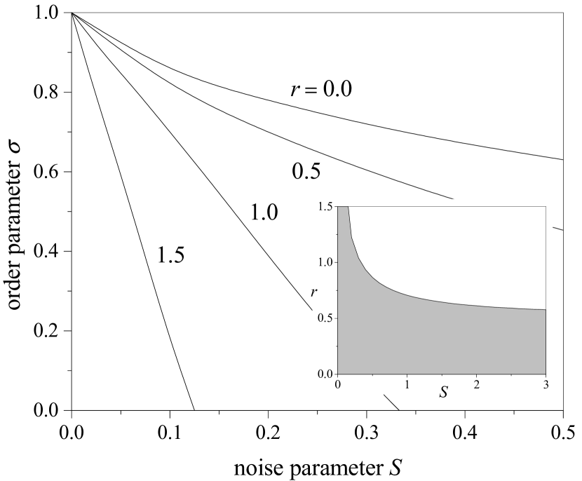
Figure 3: Kuramoto order parameter $\sigma$ as a function of the parameter $S$ in an ensemble of coupled oscillators with the distribution of coupling strengths and noise intensities given in equation (15), taking $\zeta(k)=S(1+k)^{r}$, as a function of $S$ and for several values of $r$. The inset shows the synchronization region ($\sigma\neq 0$; shaded) in the parameter plane $(S,r)$.

Our main conclusions can be summarized as follows. We have considered a heterogeneous ensemble of coupled phase oscillators subject to external fluctuations, where the coupling strength and the effect of noise can be different for each oscillator. In ensembles with homogeneous coupling synchronized behaviour emerges spontaneously, but sufficiently large homogeneous fluctuations inhibit synchronization fromcells . We have shown here that, on the other hand, homogeneous noise may not be able to inhibit synchronization if the coupling strength is not the same for all oscillators. Specifically, if the distribution of coupling strengths decays slowly enough for large couplings, synchronization persists even under arbitrarily large fluctuations. A similar, complementary effect takes place when noise intensities are in turn heterogeneous over the ensemble. An excess of oscillators with very small response to noise can suppress unsynchronized behaviour, even when the distribution of coupling strengths would allow for the desynchronization transition under large homogeneous noise. In the more generic situation where the coupling strength and the noise intensity of each oscillator are correlated, the two attributes may “control” each other. Large couplings, which favor synchronization, compete with large fluctuations, which tend to inhibit coherent behaviour. The precise form of their correlation defines whether the desynchronization transition exists or not.

Similar results were implicit in the analysis of oscillator ensembles where both natural frequencies and coupling strengths are heterogeneous, in the absence of noise pais1 ; pais2 . For instance, if the distribution of coupling strengths at the synchronization frequency decays slowly enough, the desynchronization transition induced by a sufficiently flat distribution of natural frequencies is suppressed, and synchronized dynamics persists for arbitrarily flat distributions. This provides a further example of the equivalent roles of diversity –in our case, heterogeneous natural frequencies– and noise, in the collective dynamics of large ensembles of interacting elements fromcells ; tess1 ; tess2 .

References

- (1) A.S. Mikhailov, V. Calenbuhr, From Cells to Societies (Springer, Berlin, 2002).
- (2) Y. Kuramoto, Chemical Oscillations, Waves, and Turbulence (Springer, Berlin, 1984).
- (3) A.T. Winfree, The Geometry of Biological Time (Springer, New York, 2001).
- (4) M. Barahona, L.M. Pecora, Phys. Rev. Lett. 89, 054101 (2002).
- (5) T. Nishikawa, A.E. Motter, Y.-Ch. Lai, F.C. Hoppensteadt, Phys. Rev. Lett. 91, 014101 (2003).
- (6) K. Park, S.W. Rhee, M.Y. Choi, Phys. Rev. E 57, 5030 (1998).
- (7) S.C. Manrubia, A.S. Mikhailov, D.H. Zanette, Emergence of Dynamical Order. Synchronization Phenomena in Complex Systems (World Scientific, Singapore, 2004).
- (8) G.H. Paissan, D.H. Zanette, EPL 77, 20001 (2007).
- (9) G.H. Paissan, D.H. Zanette, Physica D 237, 818 (2008).
- (10) C.W. Gardiner, Handbook of Stochastic Methods (Springer, Berlin, 1997).
- (11) M. Abramowitz, I.A. Stegun, Handbook of Mathematical Functions (Dover, New York, 1970) p. 374.
- (12) C.J. Tessone, C. Mirasso, R. Toral, J.D. Gunton, Phys. Rev. Lett. 97, 194101 (2006).
- (13) C.J. Tessone, A. Scirè, R. Toral, O. Colet, Phys. Rev. E 75, 016203 (2007).