A branch-point approximant for the equation of state of hard spheres

Abstract

Using the first seven known virial coefficients and forcing it to possess two branch-point singularities, a new equation of state for the hard-sphere fluid is proposed. This equation of state predicts accurate values of the higher virial coefficients, a radius of convergence smaller than the close-packing value, and it is as accurate as the rescaled virial expansion and better than the Padé [3/3] equations of state. Consequences regarding the convergence properties of the virial series and the use of similar equations of state for hard-core fluids in $d$ dimensions are also pointed out.

I Introduction

The virial expansion of the equation of state (EOS) is an expansion in powers of (usually) the number density $\rho$ that was originally introduced phenomenologically by Kammerlingh OnnesKO909 in 1909 in order to provide a mathematical representation of experimental data. Later, in what may be considered as one of the great achievements in statistical physics in the twentieth century, MayerMM40 was able to derive such an expansion for the pressure $p$ of a classical fluid in terms of its density. The corresponding virial coefficients (usually denoted by $B_{j}$) turn out to be related to integrals over the interaction among groups of fluid particles and are in general functions of the absolute temperature $T$. In the case of hard-sphere (HS) fluids, which are the subject of this paper, the virial coefficients are however independent of $T$. In particular, the value of the second virial coefficient for HSs in $d$ dimensions is $B_{2}=2^{d-1}v_{d}\sigma^{d}$, where $\sigma$ is the diameter of the spheres and $v_{d}=(\pi/4)^{d/2}/\Gamma(1+d/2)$ is the volume of a $d$-dimensional sphere of unit diameter, a result first derived for three-dimensional HSs ($d=3$) by van der Waals.vdW899 Analytical expressions for $B_{3}$ and $B_{4}$ are also available in the literatureJ896 ; B896 ; vL899 ; B899 ; T36 ; R64 ; H64 ; LB82 ; BC87 ; CM04a ; L05 but higher virial coefficients must be computed numerically and, since this represents a non trivial task, up to now only values up to the tenth virial coefficient have been reported.MRRT53 ; RR54 ; RH64a ; RH64b ; R65 ; RH67 ; KH68 ; K76 ; K77 ; K82a ; K82b ; vRT92 ; vR93 ; VYM02 ; CM04b ; LKM05 ; CM05 ; KR06 ; CM06 ; BCW08

The virial expansion for $d$-dimensional HS systems is often expressed in terms of the packing fraction $\eta$ defined as $\eta=v_{d}\,\rho\,\sigma^{d}$. Hence, for these systems the compressibility factor $Z\equiv p/\rho k_{B}T$ (with $k_{B}$ the Boltzmann constant) is given by

$$Z(\eta)=1+\sum_{j=2}^{\infty}b_{j}\eta^{j-1},$$ (1)

where the (reduced) virial coefficients $b_{j}\equiv B_{j}/(v_{d}\sigma^{d})^{j-1}$ are now pure numbers.

The availability of only a few virial coefficients represents a restriction on the usefulness of the virial expansion and many issues about it are still unresolved. For instance, its radius of convergence is not known eventhough lower bounds are available.LP64 ; FPS07 Secondly, although all the available virial coefficients in $d=2$, $d=3$, and $d=4$ are positive, even the character of the series (either alternating or not) is still unknown. In fact results from higher dimensions suggest that the positive character might not be true for the higher virial coefficients of hard disks and spheres.CM06 ; RMHS08 ; AKV08 Finally, people have usually recurred to approximate EOSs obtained through the knowledge of the limited number of virial coefficients via various series acceleration methods such as Padé or Levin approximants. However, the expectation that these EOSs would ultimately lead to the complete phase behavior of the system has not been fulfilled. Hence, the question of whether the virial series contains relevant information related to the phase behavior of the HS system also remains as an open one.

Recently it has been clearly established that the EOSs for hard hyperspheres ($d\geq 4$) predicted by the Percus–Yevick (PY) integral equation possess a branch-point singularity on the negative real axis that is responsible for the radius of convergence and the alternating character of the virial series.RMHS08 ; AKV08 It is very likely that these features are not artifacts of the PY approximation but would be shared by the exact EOSs. However, in the case of hard spheres ($d=3$), the radius of convergence of the PY EOS is artificially $\eta=1$ and, as stated above, there is no definite indication about the nature of the singularity responsible for the true radius of convergence or its value.CM06

The main aim of this paper is to shed some more light on the character of the virial series of the three-dimensional HS fluid. The idea is to propose a new (heuristic) EOS for HS systems in $d$ dimensions that, for reasons that will become clear later, we will refer to as a ‘branch-point approximant.’ Such a proposal is not geared specifically towards obtaining an accurate EOS but rather relies on the notion that the radius of convergence of the virial series might be dictated by a branch-point singularity. In any case, the plausibility of this notion will be assessed by comparing the predictions of high virial coefficients coming out of the proposal both with the exact values of these coefficients for each $d$ and with the performance of other proposals for the EOS (rescaled virial expansions and Padé approximants).

The paper is organized as follows. In the next section we introduce the new EOS including a branch-point singularity and examine the case of three-dimensional HSs. Section III refers to the use of the same type of EOS for different dimensionalities. We close the paper in Sect. IV with some discussion and concluding remarks.

II The case of hard spheres ($d=3$)

We begin by proposing a ‘branch-point approximant’ for the EOS of $d$-dimensional HS systems, namely

$$Z(\eta)=1+\frac{1+c_{1}\eta+c_{2}\eta^{2}+c_{3}\eta^{3}-\left(1+2a_{1}\eta+a_{2}\eta^{2}\right)^{3/2}}{A(1-\eta)^{k}},$$ (2)

where $A$, $a_{1}$, $a_{2}$, $c_{1}$, $c_{2}$, $c_{3}$, and $k$ are parameters to be determined. This functional form (with $k=3$) is inspired by the EOS for hard hyperspheres in $d=5$ predicted by the PY theory through the virial route.FI81 ; L84 ; GGS90 ; BMC99 As stated above, we will assume the approximant form given in Eq. (2) for three-dimensional HSs as a toy model to highlight the possibility that the radius of convergence of the virial series in this system might be dictated by a branch-point singularity. According to the philosophy of an approximant, the six coefficients $A$, $a_{1}$, $a_{2}$, $c_{1}$, $c_{2}$, and $c_{3}$ are obtained from the knowledge of the virial coefficients $b_{2}$–$b_{7}$. The resulting expressions are given in Table 1, where we have called

$$S_{k,n}\equiv\sum_{j=2}^{n}\binom{k}{n-j}(-1)^{j}b_{j}.$$ (3)

Table 1: Expressions (for general $k$) and numerical values (for $k=d=3$) of $a_{1}$, $a_{2}$, $A$, and $c_{1}$–$c_{3}$.

Coefficient	Expression	Value
$a_{1}$	${S_{k,6}}/{S_{k,5}}$	$0.271232$
$a_{2}$	$7a_{1}^{2}-6{S_{k,7}}/{S_{k,5}}$	$1.94804$
$A$	$\frac{3}{8}{(a_{2}-a_{1}^{2})^{2}}/{S_{k,5}}$	$1.51486$
$c_{1}$	$3a_{1}+b_{2}A$	$6.87314$
$c_{2}$	$\frac{3}{2}(a_{2}+a_{1}^{2})-S_{k,3}A$	$0.00268343$
$c_{3}$	$\frac{1}{2}a_{1}(3a_{2}-a_{1}^{2})+S_{k,4}A$	$1.33515$

Although the choice for $k$ is in principle arbitrary, a natural one seems to take $k=d$. Hence, in this Section we assume $k=3$. A special situation takes place if $a_{2}=a_{1}^{2}$. In that case, the denominator ($S_{3,5}$) in the expression for $A$ must vanish in order to have a finite value, i.e., $b_{5}=b_{2}-3b_{3}+3b_{4}$. Since this denominator also appears in the expressions for $a_{1}$ and $a_{2}$, the respective numerators ($S_{3,6}$ and $S_{3,7}$) must also vanish, i.e., one must have $b_{6}=3b_{2}-8b_{3}+6b_{4}$ and $b_{7}=6b_{2}-15b_{3}+10b_{4}$. Under those conditions, one has $c_{1}=3a_{1}+b_{2}A$, $c_{2}=3a_{1}^{2}-S_{3,3,}A$, $c_{3}=a_{1}^{3}+S_{3,4}A$, so that Eq. (2) becomes $Z(\eta)=1+\eta\left[b_{2}+(b_{3}-3b_{2})\eta+(b_{4}-3b_{3}+3b_{2})\eta^{2}\right]/(1-\eta)^{3}$, regardless of the values of $a_{1}$ and $A$. The aforementioned relationships are precisely satisfied by the virial and compressibility routes to the EOS in the PY approximation for $d=3$. Therefore, the functional form (2) is general enough as to include both PY EOSs, and thus also the Carnahan–Starling (CS) EOS,CS69 given by

$$Z_{\text{CS}}(\eta)=\frac{1+\eta+\eta^{2}-\eta^{3}}{(1-\eta)^{3}},$$ (4)

as particular cases. Moreover, in the one-dimensional case one has $b_{j}=1$, so that again the relationships are satisfied and the resulting compressibility factor reduces to the exact EOS of the system, namely $Z(\eta)=1/(1-\eta)$.

The numerical values of the coefficients $a_{1}$, $a_{2}$, $A$, and $c_{1}$–$c_{3}$ obtained from the known values of the first seven virial coefficientsLKM05 ; CM06 (namely, $b_{2}=4$, $b_{3}=10$, $b_{4}\simeq 18.364768$, $b_{5}\simeq 28.2245$, $b_{6}\simeq 39.8151$, $b_{7}\simeq 53.3444$) are given in Table 1. The two branch points $-(a_{1}\pm\sqrt{a_{1}^{2}-a_{2}})/a_{2}=-0.139234\pm 0.702817i$ lie on the complex plane. Their modulus is $1/\sqrt{a_{2}}=0.716$ and this is then the radius of convergence of the virial series of the EOS (2). While this radius is possibly an overestimate (in fact, it is larger than the freezing density), it is not unphysical since it is smaller than the close-packing value, in contrast to the radius $\eta=1$ given by the PY, the CS, and the Carnahan–Starling–Kolafa (CSK)Kolafa EOSs, to name just a few.

Table 2: Exact and predicted values of $b_{8}$–$b_{10}$ in the three-dimensional case

. Coefficient Exact Branch-point Rescaled expansion Padé [3/3] Eq. (2), $k=3$ Eq. (5), $m=6$, $k=3$ Eq. (6) $b_{8}$ $68.538$ $68.609$ $68.812$ $69.040$ $b_{9}$ $85.813$ $85.532$ $86.219$ $87.147$ $b_{10}$ $105.78$ $104.32$ $105.56$ $107.93$

Table 2 compares the knownLKM05 ; CM06 and predicted values of $b_{8}$–$b_{10}$. Apart from the values predicted by Eq. (2), the table also includes the values obtained from the two following approximate EOSs that also make use of $b_{2}$–$b_{7}$: the rescaled virial expansionBC87

$$Z=\frac{1+\sum_{n=1}^{m}C_{n}\eta^{n}}{(1-\eta)^{k}},$$ (5)

where $m=6$, $k=3$, and $C_{n}=(-1)^{n}\left[\binom{k}{n}-S_{k,n+1}\right]$, with $S_{k,n}$ given by Eq. (3), and the bestGB08 Padé approximant [3/3] given by

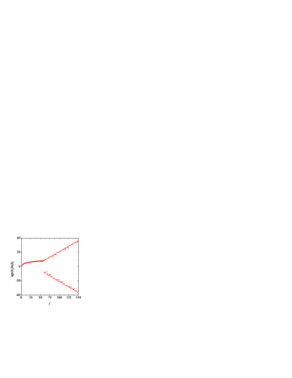
Figure 1: (Color online) Plot of $\text{sgn}(b_{j})\ln|b_{j}|$ for $j\leq 150$ in the three-dimensional case.

$$Z=\frac{1+\sum_{n=1}^{3}D_{n}\eta^{n}}{1+\sum_{n=1}^{3}E_{n}\eta^{n}}.$$ (6)

where $D_{n}$ and $E_{n}$ ($n=1,2,3$) are combinations of $b_{2}$–$b_{7}$ whose explicit expressions may be easily obtained but will be omitted here. The deviations from the correct ones of the values for $b_{8}$–$b_{10}$ predicted by Eq. (2) are $0.1\%$, $0.3\%$, and $1.4\%$, respectively. In contrast, the deviations of the values predicted by the rescaled virial expansion and the Padé approximant [3/3] are $0.4\%$, $0.5\%$, and $0.2\%$ and $0.7\%$, $1.5\%$, and $2\%$, respectively. Note that, in particular, the rescaled virial expansion predicts a very accurate value for $b_{10}$, even better than the prediction for $b_{8}$. At a qualitative level, an interesting outcome of Eq. (2) is first that it predicts a negative value of a certain coefficient (specifically, $b_{59}$) and secondly that henceforth the coefficients change sign every 1-2 terms. Figure 1 shows $\text{sgn}(b_{j})\ln|b_{j}|$ for $j\leq 150$. In contrast, the rescaled virial expansion predicts that all the $b_{j}$ are positive, while the Padé [3/3] predicts positive coefficients up to $b_{56}$ and then alternating signs for groups of $55$ consecutive coefficients.

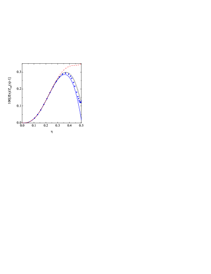
Figure 2: (Color online) Plot of $100[Z(\eta)/Z_{\text{CS}}(\eta)-1]$ in the three-dimensional case. Solid line: $Z(\eta)$ given by the branch-point approximant (2) with $k=3$; dotted line: $Z(\eta)$ given by the rescaled virial approximant (5) with $m=6$ and $k=3$; dashed line: $Z(\eta)$ given by the Padé [3/3] approximant (6). The circles are simulation data from Ref. KLM04, .

While the comparison between the exact values of the higher reduced virial coefficients and those that follow from the expansion of Eq. (2) is quite satisfactory, one may reasonably wonder how the new EOS will perform when compared with other accurate proposals. Figure 2 shows that both the branch-point approximant and the rescaled virial expansion deviate less than $0.3\%$ from the CS values for $0\leq\eta\leq 0.5$ and are in very good agreement with simulation dataKLM04 . The Padé [3/3] does a poorer job in this instance. Hence, the performance of the new proposal is also very accurate over the whole fluid phase range.

III Other dimensionalities

In this Section we perform a similar analysis of the use of Eq. (2) with $k=d$ for all the dimensionalities ($d=2,4,5,6,7,8,$ and $9$) where the first ten virial coefficients are known.CM06 ; BCW08

Table 3: Exact and predicted values of $b_{8}$–$b_{10}$ for $d=2$ and $d=4$–$9$

. Coefficient Exact Branch-point Rescaled expansion Padé [3/3] Eq. (2), $k=d$ Eq. (5), $m=6$, $k=d$ Eq. (6) $d=2$ $b_{8}$ $8.3191$ $8.3397$ $8.3408$ $8.3241$ $b_{9}$ $9.2721$ $9.3711$ $9.3297$ $9.3001$ $b_{10}$ $10.216$ $10.469$ $10.319$ $10.298$ $d=4$ $b_{8}$ $605.66$ $284.49$ $486.07$ $543.55$ $b_{9}$ $739.88$ $3339.4$ $562.33$ $605.51$ $b_{10}$ $1516.7$ $-5388.0$ $579.18$ $704.91$ $d=5$ $b_{8}$ $-3.0064\times 10^{4}$ $-3.0177\times 10^{4}$ $3.1662\times 10^{4}$ $-2.6584\times 10^{4}$ $b_{9}$ $3.2083\times 10^{5}$ $3.1961\times 10^{5}$ $9.4841\times 10^{4}$ $2.3254\times 10^{5}$ $b_{10}$ $-3.3810\times 10^{6}$ $-2.9014\times 10^{6}$ $2.2311\times 10^{5}$ $-1.6907\times 10^{6}$ $d=6$ $b_{8}$ $-3.0752\times 10^{7}$ $-3.0448\times 10^{7}$ $9.4362\times 10^{6}$ $-2.6002\times 10^{7}$ $b_{9}$ $7.3370\times 10^{8}$ $7.1562\times 10^{8}$ $3.42934\times 10^{7}$ $5.0061\times 10^{8}$ $b_{10}$ $-1.8472\times 10^{10}$ $-1.7587\times 10^{10}$ $9.3201\times 10^{7}$ $-9.5796\times 10^{9}$ $d=7$ $b_{8}$ $-8.7684\times 10^{9}$ $-8.6759\times 10^{9}$ $1.3044\times 10^{9}$ $-7.6577\times 10^{9}$ $b_{9}$ $4.7482\times 10^{11}$ $4.6063\times 10^{11}$ $5.3315\times 10^{9}$ $3.3839\times 10^{11}$ $b_{10}$ $-2.7274\times 10^{13}$ $-2.5651\times 10^{13}$ $1.6168\times 10^{10}$ $-1.4941\times 10^{13}$ $d=8$ $b_{8}$ $-1.6114\times 10^{12}$ $-1.5950\times 10^{12}$ $1.2461\times 10^{11}$ $-1.4369\times 10^{12}$ $b_{9}$ $1.8713\times 10^{14}$ $1.8107\times 10^{14}$ $5.6751\times 10^{11}$ $1.3783\times 10^{14}$ $b_{10}$ $-2.3160\times 10^{16}$ $-2.1589\times 10^{16}$ $1.9031\times 10^{12}$ $-1.3220\times 10^{16}$ $d=9$ $b_{8}$ $-2.3219\times 10^{14}$ $-2.2913\times 10^{14}$ $9.6059\times 10^{12}$ $-2.0919\times 10^{14}$ $b_{9}$ $5.5879\times 10^{16}$ $5.3746\times 10^{16}$ $4.8352\times 10^{13}$ $4.1962\times 10^{16}$ $b_{10}$ $-1.4436\times 10^{19}$ $-1.3252\times 10^{19}$ $1.7789\times 10^{14}$ $-8.4195\times 10^{18}$

Table 3 displays the exact and predicted values of $b_{8}$–$b_{10}$ for $d=2$ and $d=4$–$9$ as given by the branch-point approximant, the rescaled virial expansion and the Padé [3/3] EOSs.

For $d=2$ the best approximant is the Padé [3/3]. The branch-point approximant also does a good job in the case of hard disks, but the rescaled virial approximation is slightly better (except for the value of $b_{8}$). The case $d=4$ is somewhat peculiar because the predictions from all the approximants are rather poor. In any event, the Padé [3/3] gives the ‘best’ performance, followed by the rescaled virial expansion, and finally the branch-point approximant. This latter even ‘anticipates’ the likely aternating character of the series and predicts a negative value of $b_{10}$. The situation changes for $5\leq d\leq 9$ where the performance of the rescaled virial expansion is extremely poor and in fact it never predicts negative coefficients, even when the exact $b_{6}<0$ is introduced ($d=6$, $d=7$) or the exact $b_{4}<0$ and $b_{6}<0$ are introduced ($d=8$, $d=9$). On the other hand, in these dimensionalities the Padé [3/3] predicts the right signs, while the branch-point approximant predicts, in addition, very good values.

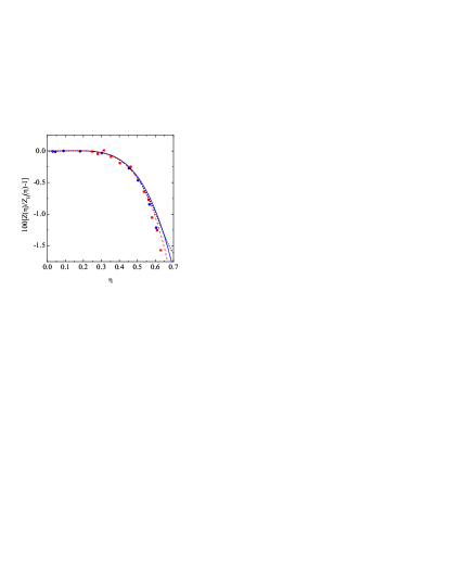
Figure 3: (Color online) Plot of $100[Z(\eta)/Z_{\text{H}}(\eta)-1]$ in the two-dimensional case. Solid line: $Z(\eta)$ given by the branch-point approximant (2) with $k=2$; dotted line: $Z(\eta)$ given by the rescaled virial approximant (5) with $m=6$ and $k=2$; dashed line: $Z(\eta)$ given by the Padé [3/3] approximant (6). The circles and squares are simulation data from Refs. EL85, and L01, , respectively.

With regards to the EOS of hard disks, in Fig. 3 we compare the performance of the different approximants with respect to the simulation dataEL85 ; L01 in the range $0\leq\eta\leq 0.7$. Note that in this range the new proposal is able to capture the deviations (of up to $2\%$) of the simulation results that one gets from the use of the reasonably accurate EOS due to Henderson,H75 namely

$$Z_{\text{H}}(\eta)=\frac{1+\eta^{2}/8}{(1-\eta)^{2}}.$$ (7)

Table 4: Singularity closest to the origin and radius of convergence of the virial series, as predicted by the branch-point approximant (2) with $k=d$. The radius predicted by the PY integral equation is also included.

$d$	Singularity	Radius	Radius (PY)
$2$	$0.3234\pm 0.4533i$	$0.557$	$1$
$3$	$-0.1392\pm 0.7028i$	$0.716$	$1$
$4$	$-0.044223\pm 0.07526i$	$0.0873$	$0.15$
$5$	$-0.07838$	$0.0784$	$0.057$
$6$	$-0.02960$	$0.0296$	$0.024$
$7$	$-0.01302$	$0.0130$	$0.011$
$8$	$-0.006062$	$0.00606$	$0.0051$
$9$	$-0.002925$	$0.00292$	$0.0024$

Concerning the nature of the singularities in these dimensions, in Table 4, we present the values of the singularity closest to the origin and the radius of convergence of the corresponding virial series, as predicted by the branch-point approximant (2) with $k=d$. For comparison, the radius predicted by the PY integral equation is also included in this table. One finds that the new proposal predicts complex branch points for $2\leq d\leq 4$. These are precisely the cases where all the known virial coefficients are positive. On the other hand, for $5\leq d\leq 9$ the branch point closest to the origin is a negative real value. This agrees with the PY results, which gives some support to the alternating series scenario. Also note that the branch-point approximant and the PY radii of convergence tend to agree as $d$ increases.

IV Concluding remarks

In this paper we have introduced a new proposal for the EOS of a three-dimensional HS fluid which is built from the knowledge of the first seven virial coefficients and possesses two branch-point singularities in the complex plane. Although the choice we have made may appear to a certain extent arbitrary, it is perhaps the simplest one embodying the PY and CS EOSs for HSs in three dimensions as well as the exact $Z$ in $d=1$ and the PY virial EOS in $d=5$. The same functional form was also assumed for the EOS of HS fluids in other dimensions. For $d=3$ the new EOS predicts accurate values of the higher virial coefficients, a radius of convergence smaller than the close-packing value, and, irrespective of the fact that its construction did not aim at accuracy, it is very accurate when compared to simulation results and with other approximants involving the same number of known virial coefficients. This last feature was shown to be also shared by the two-dimensional case. The proposal is also robust with respect to small ($\sim 1\%$) deviations in the value of the seventh virial coefficient, certainly more robust than either the rescaled virial expansion or the Padé [3/3].

Except for $d=4$ (where, as already pointed out by Clisby and McCoyCM06 in a somewhat related context, perhaps one would require better accuracy of the known virial coefficients), in all other dimensionalities the branch-point approximant gives the best overall performance with respect to the prediction of the known virial coefficients. In particular, the rescaled virial expansion is unable to predict even the signs of known virial coefficients for $d\geq 5$ and the Padé [3/3], although correctly capturing these signs, leads to higher deviations. This of course constitutes no proof that the true EOS of HS systems should include a branch-point singularity, but the evidence provided here is at least consistent with it.

On a related vein, the new EOS for HSs in $d=3$ also leads to an alternating virial series, with $b_{59}$ being the first negative reduced virial coefficient. Given the difficulty of computing exact high order virial coefficients, it is unlikely that the alternating series scenario for HSs in three dimensions may be confirmed in the near future. However, in view of the present results and those obtained in higher dimensions,CM06 ; RMHS08 ; AKV08 it certainly gets reinforced.

One can reasonably wonder whether the present approach to construct the EOS of HS systems using a number of known virial coefficients may be cast in a systematic way. While the answer is certainly not unique, the following constitutes a possible generalization. We rewrite the compressibility factor as

$$Z(\eta)=1+\frac{1+\sum_{n=1}^{2N+1}c_{n}\eta^{n}-\left(1+2a_{1}\eta+a_{2}\eta^{2}\right)^{N+1/2}}{A(1-\eta)^{k}},$$ (8)

where taking $N=1$ corresponds to Eq. (2). In the three-dimensional case ($k=d=3$), the approximant with $N=0$ (which amounts to including only the first five virial coefficients) predicts $b_{6}$–$b_{10}$ with deviations equal to $0.54\%$, $0.69\%$, $1.2\%$, $3\%$, and $5\%$, respectively. On the other hand, the approximant with $N=2$ predicts $b_{10}$ with a $1.2\%$ deviation. Therefore, although there is certainly an improvement in the prediction of $b_{10}$ on going from $N=0$ to $N=2$, a reasonable compromise between simplicity, generality, and accuracy seems to suggest that the choice $N=1$ is the most adequate.

Finally, it should be pointed out that if instead of choosing $k=d$ as we have done in this paper, a different $k$ is picked (say $k=3$ for all $d$) we find slight variations in the numerical predictions but the overall picture remains unaltered.

- (1) H. Kammerlingh Onnes, Commun. Leiden 71 (1909).
- (2) J. E. Mayer and M. G. Mayer, Statistical Mechanics, (Wiley, N.Y., 1940). Chapter 13.
- (3) J. D. van der Waals, Proc. Kon. Acad. V. Wetensch, Amsterdam, 1, 138 (1899).
- (4) G. Jäger, Sitzber. Akad. Wiss. Wien, Math. Natur-w. Kl. (Part 2a) 105, 15 (1896).
- (5) L. Boltzmann, Sitzber. Akad. Wiss. Wien, Math. Natur-w. Kl. (Part 2a) 105, 695 (1896).
- (6) J. J. van Laar, Proc. Konikl. Acad. Wetensch., Amsterdam 1, 273 (1899).
- (7) L. Boltzmann, Proc. Konikl. Acad. Wetensch., Amsterdam 1, 398 (1899).
- (8) L. Tonks, Phys. Rev. 50, 955 (1936).
- (9) J. S. Rowlinson, Mol. Phys. 7, 593 (1964).
- (10) P. C. Hemmer, J. Chem. Phys. 42, 1116 (1964).
- (11) M. Luban and A. Baram, J. Chem. Phys. 76, 3233 (1982).
- (12) M. Baus and J. L. Colot, Phys. Rev. A 36, 3912 (1987).
- (13) N. Clisby and B. M. McCoy, J. Stat Phys. 114, 1343 (2004).
- (14) I. Lyberg, J. Stat Phys. 119, 747 (2005).
- (15) N. Metropolis, A. W. Rosenbluth, M. N. Rosenbluth, and A. H. Teller, J. Chem. Phys. 21, 1087 (1953).
- (16) M. N. Rosenbluth and A. W. Rosenbluth, J. Chem. Phys. 22, 881 (1954).
- (17) F. H. Ree and W. G. Hoover, J. Chem. Phys. 40, 939 (1964).
- (18) F. H. Ree and W. G. Hoover, J. Chem. Phys. 41, 1635 (1964).
- (19) J. S. Rowlinson, Rep. Progr. Phys. 28, 169 (1965).
- (20) F. H. Ree and W. G. Hoover, J. Chem. Phys. 46, 4181 (1967).
- (21) S. Kim and D. Henderson, Phys. Lett. A 27, 378 (1968).
- (22) K. W. Kratky, Physica A 85, 607 (1976).
- (23) K. W. Kratky, Physica A 87, 548 (1977).
- (24) K. W. Kratky, J. Stat Phys. 27, 533 (1982).
- (25) K. W. Kratky, J. Stat Phys. 29, 129 (1982).
- (26) E. J. Janse van Rensburg and G. M. Torrie, J. Phys. A: Math. Gen. 26, 943 (1992).
- (27) E. J. Janse van Rensburg, J. Phys. A: Math. Gen. 26, 4805 (1993).
- (28) A. Y. Vlasov, X. M. You, and A. J. Masters, Mol. Phys. 100, 3313 (2002).
- (29) N. Clisby and B. M. McCoy, J. Stat Phys. 114, 1361 (2004).
- (30) S. Labík, J. Kolafa, and A. Malijevský, Phys. Rev. E 71, 021105 (2005).
- (31) N. Clisby and B. M. McCoy, Pramana 64, 775 (2005).
- (32) J. Kolafa and M. Rottner, Mol. Phys. 104, 3435 (2006).
- (33) N. Clisby and B. M. McCoy, J. Stat Phys. 122, 15 (2006).
- (34) M. Bishop, N. Clisby, and P. A. Whitlock, J. Chem. Phys. 128, 034506 (2008).
- (35) J. L. Lebowitz and O. Penrose, J. Math. Phys. 5, 841 (1964).
- (36) R. Fernández, A. Procacci and B. Scoppola, J. Stat Phys. 128, 1139 (2007).
- (37) R. D. Rohrmann, M. Robles, M. López de Haro, and A. Santos, J. Chem. Phys. 129, 014510 (2008).
- (38) M. Adda-Bedia, E. Katzav, and D. Vella, J. Chem. Phys. 129, 144506 (2008).
- (39) C. Freasier and D. J. Isbister, Mol. Phys. 42, 927 (1981).
- (40) E. Leutheusser, Physica A 127, 667 (1984).
- (41) D. J. González, L. E. González, and M. Silbert, Phys. Chem. Liq. 22, 95 (1990).
- (42) M. Bishop, A. Masters, and J. H. R. Clarke, J. Chem. Phys. 110, 11449 (1999).
- (43) N. F. Carnahan and K. E. Starling, J. Chem. Phys. 51, 635 (1969).
- (44) This EOS is a slight modification by J. Kolafa of the CS EOS. It first appeared as Eq. (4.46) in the review paper by T. Boublík and I. Nezbeda, Collect. Czech. Chem. Commun. 51, 2301 (1986).
- (45) A. O. Guerrero and A. B. M. S. Bassi, J. Chem. Phys. 129, 044509 (2008).
- (46) J. Kolafa, S. Labík, and A. Malijevský, Phys. Chem. Chem. Phys. 6, 2335 (2004).
- (47) J. J. Erpenbeck and M. Luban, Phys. Rev. A 32, 2920 (1985).
- (48) S. Luding, Phys. Rev. E 63, 042201 (2001); Adv. Compl. Syst. 4, 379 (2002), reprinted in Challenges in Granular Physics, edited by T. Halsey and A. Mehta (World Scientific, Singapore, 2002), pp. 91–100; in The Physics of Granular Media, edited by H. Hinrichsen and D. Wolf, (Wiley-VCH, Berlin, 2004), Chap. 13.
- (49) D. Henderson, Mol. Phys. 30, 971 (1975).