The Wigner Function of Produced Particles in String Fragmentation

Abstract

We show that QCD4 with transverse confinement can be approximately compactified into QCD2 with a transverse quark mass $m_{{}_{T}}$ that is obtained by solving a set of coupled transverse eigenvalue equations. In the limits of a strong coupling and a large number of flavors, QCD2 further admits Schwinger QED2-type bosonized solutions. We therefore examine phenomenologically the space-time dynamics of produced particles in string fragmentation by studying the Wigner function of produced bosons in Schwinger QED2, which mimics many features of string fragmentation in quantum chromodynamics. We find that particles with momenta in different regions of the rapidity plateau are produced at the initial moment of string fragmentation as a quark pulls away from an antiquark at high energies, in contrast to classical pictures of string fragmentation with longitudinal space-momentum-time ordering.

I Introduction

Soft particle production by string fragmentation is an important process in high energy collisions. In the strongly-coupled regime in nucleus-nucleus collisions at RHIC energies, the dynamics of string fragmentation falls within the realm of non-perturbative quantum chromodynamics (QCD), and the detailed mechanism of the production process cannot yet be described from the first principles of QCD. Phenomenological particle production models based on preconfinement Wol80 , parton-hadron duality Van88 cluster fragmentation Odo80 , string-fragmentation And83 , dual-partons Cap78 , the Venus model Wer88 , the RQMD model Sor89 , multiple collision model Won89 , parton cascade model Wan94 ; Gei92 , color-glass condensate model McL94 , the AMPT model Li96 , the Lexus model Jeo97 , and many other models have been put forth and are successful in describing some aspects of the data. These models incorporate some features of QCD, but their fundamental foundation in non-perturbative QCD is still lacking. It is of interest to study the physics of particle production in string fragmentation with QCD-inspired, low-dimensional non-perturbative models.

Two-dimensional quantum electrodynamics Sch62 ; Low71 ; Col75 ; Col76 ; Cas74 ; Bjo83 ; Ili84 ; Ell87 ; Fuj89 ; Won91 ; Won94 in one space and one time coordinates (QED2) furnishes an interesting arena for such a study. This is a quantum mechanical system in which a fermion interacts with an antifermion through a linear gauge field potential in the Coulomb gauge. It is a system where the Higgs phenomenon occurs and the global chiral symmetry is spontaneously broken Sch62 ; Low71 ; Col75 ; Col76 . When a positive fermion and a negative antifermion are separated in such a system, the vacuum is so polarized that the positive and the negative charges are completely screened, in a manner similar to the confinement of quarks. The quantum field theory of massless fermions interacting with a gauge field in QED2 can be solved exactly Sch62 ; Low71 ; Col75 ; Col76 ; Cas74 ; Bjo83 . The interacting field turns out to be equivalent to the quantum field theory of free bosons with a mass. It was demonstrated by Casher, Kogut and Susskind Cas74 that when a fermion separates from an antifermion in the limit of infinite energies in QED2, the rapidity distribution of the produced particles will exhibit the property of boost invariance. For a finite energy system, the boost-invariant solution turns naturally into a rapidity plateau, whose width increases with energy as $\ln(\sqrt{s})$ Won91 ; Won94 .

Rapidity plateau distributions of produced particles have indeed been observed in high-energy $e^{+}$-$e^{-}$ annihilation which produces initially a separating quark and an antiquark Aih88 ; Hof88 ; Aihnote ; Pet88 ; Abe99 ; Abr99 . Rapidity plateau distributions of produced particles have also been observed in $pp$ collisions at $\sqrt{s}=200$ GeV by the BRAHMS Collaboration Yan08 . The close similarities of the features of empirical fragmentation data and theoretical QED2 fragmentation results motivate us to examine in this paper the circumstances in which the longitudinal dynamics of a transversely-confined QCD4 system can be approximately compactified into QCD2. We also need to examine further how multi-flavor QCD2 can be approximated by QED2.

Our renewed interest in the non-perturbative production mechanism arises from the puzzling observations of the momentum distribution of particles associated with a near-side jet. In high-energy heavy-ion collisions, a near-side jet is characterized by the presence of associated particles within a narrow cone along the trigger particle direction. Its characteristics resemble those of a jet in $pp$ and peripheral heavy-ion collisions. In addition to this ‘jet component’, there is an additional ‘ridge component’ of associated particles at $\Delta\phi$$\sim$0 with a ridge structure in $\Delta\eta$, where $\Delta\phi$ and $\Delta\eta$ are the azimuthal angle and pseudorapidity differences measured relative to the trigger particle Ada05 ; Ada06 ; Put07 ; Bie07 ; Wan07 ; Bie07a ; Abe07 ; Mol07 ; Lon07 ; Nat08 ; Fen08 ; Net08 ; Bar08 ; Dau08 ; Ada08 ; Mcc08 ; Che08 ; Wen08 ; Tan08 ; Jia08qm ; Lee08 .

In the phenomenon of the ridge associated with the near-side jet, it is observed that (i) the ridge particle yield increases with the number of participants, (ii) the ridge yield appears to be nearly independent of the trigger jet properties, (iii) the baryon to meson ratios of the ridge particles are more similar to those of the bulk matter than those of the jet, and (iv) the slope parameter of the transverse distribution of ridge particles is intermediate between those of the jet and the bulk matter Ada05 -Lee08 . These features suggest that the ridge particles are medium partons, at an earlier stage of the medium evolution during the passage of the jet. The azimuthal correlation of the ridge particle with the jet and the presence of strong screening suggest that the associated ridge particle and the trigger jet are related by a collision. A momentum kick model was put forth to explain the ridge phenomenon Won07 ; Won07a ; Won08 ; Won08a ; Won09 . The model assumes that a near-side jet occurs near the surface, collides with medium partons, loses energy along its way, and fragments into the trigger and its associated fragmentation products (the “jet component”). Those medium partons that collide with the jet acquire a longitudinal momentum kick along the jet direction. They subsequently materialize by parton-hadron duality as ridge particles in the “ridge component”. They carry direct information on the momentum distribution of the medium partons at the moment of jet-(medium parton) collisions. Based on such a description, the experimental ridge data of the STAR, PHOBOS, and PHENIX Collaborations Ada05 ; Put07 ; Wan07 ; Wen08 ; Ada08 reveal an early parton momentum distribution that has a thermal-like transverse momentum distribution and a rapidity plateau extending to rapidities as large as $|y|\sim 4$.

The early stage of a nucleus-nucleus collision consists of simultaneous particle production processes involving quarks pulling away from antiquarks (or $qq$ diquarks) at high energies. As experimental data of elementary production processes have a rapidity plateau structure Aih88 ; Hof88 ; Aihnote ; Pet88 ; Abe99 ; Abr99 ; Yan08 , partons at the early stage of the nucleus-nucleus collision can possess the characteristics of a rapidity plateau. A rapidity plateau would also be expected from the theoretical model of string fragmentation in QED2 Cas74 ; Bjo83 ; Won91 ; Won94 , the dual-parton model Cap78 , the Bjorken hydrodynamics Bjo83 , the Lund model And83 , the Venus model Wer88 , color-glass condensate model McL94 , the Lexus model Jeo97 , and many other models. Thus, the possibility of a rapidity plateau for the ridge particles should not come as a surprise. However, the fact that a parton of large absolute rapidity can occur together with a jet of central rapidities, as revealed by the PHOBOS data and the momentum kick model analysis, poses an interesting conceptual question. For those medium partons with large magnitude of the longitudinal momentum to collide with the jet so as to become an associated ridge particle in the PHOBOS experiment, the partons must be present in the longitudinal neighborhood of the jet at the moments of the jet-medium collision, at an early stage of the nucleus-nucleus collision.

In many classical descriptions of particle production processes, a particle with a large absolute rapidity is associated with a large separation from the longitudinal origin. For example, in the Lund model of string fragmentation And83 , there is a momentum-space-time ordering of produced particles in the fragmentation of a string. Consider the case in the center-of-mass system. Those particles with the smallest absolute rapidity will be produced nearest to the origin at the earliest times, while those with the largest absolute rapidity will be produced farthermost from the origin at the latest times And83 ; Won94 .

In Bjorken hydrodynamics Bjo83 , the spatial configurations are invariant with respect to a boost in rapidity. There is a longitudinal momentum-space ordering of the produced particles. Particles at the local longitudinal location $z=0$ have rapidity zero and it is necessary to go to a relatively large absolute longitudinal coordinate $|z|$ to find another particle with a large absolute rapidity $|y|$.

In another classical model of Landau hydrodynamics Lan53 ; Won08Lan1 ; Won08Lan2 , one starts with a fluid initially at rest. As the fluid evolves, there is also an ordering of the rapidity with the longitudinal coordinate and time. It is necessary to go to larger absolute longitudinal coordinates at later times to find particles with larger absolute rapidities.

In these classical pictures of produced particles, there is a space-momentum-time ordering. Those partons with large values of absolute rapidities are not produced at the early stage of the jet production and therefore cannot be associated with a jet by a collision. On the other hand, the PHOBOS data Wen08 and the momentum kick model analysis Won07 ; Won07a ; Won08 ; Won08a ; Won09 indicate that a central rapidity jet and another parton at a large absolute rapidity can be associated by a collision. How does one resolve the difference of these two seemingly contradicting results?

It should be pointed out that the momentum-space-time ordering of produced particles in the above classical descriptions is obtained in final-state-interaction models. There is however another class of well-justified initial-state-interaction models, in which the constituent particles or produced particles are present at or before the collision process at $t=0$. Notable examples are the parton model Fey69 and the Drell-Yan process Dre71 , which assume the presence of constituent partons inside the hadron or in the quark-antiquark sea before collisions. The multi-peripheral model Che68 assumes the exchange of a tower of reggeons and the plateau of particles are present before the collision at $t$=0. The dipole approach in photon-induced reactions Huf00 assumes the fluctuation of the incident photon into a dipole quark-antiquark pair before its collision with the hadron.

With regard specifically to the dynamics of produced particles in the fragmentation of a string, it is important to point out that there are important quantum effects Jor35 ; Sch62 ; Ili84 arising from the vacuum structure in strongly-coupled non-perturbative quantum field theories that are beyond the realm of classical considerations. The proper space-time dynamics should be based on a quantum field theory where the quantum effects of the vacuum structure play appropriate roles. As is well known, in theories where the fermions are weakly interacting and can be isolated, the bare vacuum suffices for the description of the dynamics in a weak-coupling perturbation theory. In contrast, however, in our systems with strong coupling between fermions, such as in massless QED2 and similar field theories, the vacuum of the filled Dirac sea is the appropriate vacuum which participates in the dynamics. The self-consistent dynamics of the filled Dirac sea in the non-perturbative response to the presence of gauge field and fermion disturbances lead to peculiar quantum effects of the axial anomaly Jor35 ; Col75 ; Col76 ; Ili84 , the confinement of the fermion Sch62 , and the appearance of massive bosons Sch62 . The particle production process in string fragmentation should therefore be treated in a non-perturbative quantum field theory framework.

While a complete non-perturbative theory based on full quantum chromodynamics is desirable, it is however not available. Simplifying approximations are needed. We shall show that a system of transversely-confined QCD4 can be approximately compactified to a system of QCD2 with a transverse quark mass $m_{{}_{T}}$ that is obtained from a set of coupled transverse eigenvalue equations. We shall show that in the limit of strong coupling and large number of flavors, a multi-flavor massless QCD2 admits Schwinger QED2-type solutions with an effective coupling constant that depends on the number of flavors. In the absence of rigorous non-perturbative QCD4 solutions, we are therefore justified to examine phenomenologically the dynamics of the system in the solvable quantum field theory of QED2, on accounts of its close theoretical connection with the transversely-confined QCD4 and its desirable properties of the proper high-energy rapidity plateau behavior, confinement, charge screening, and chiral symmetry breaking.

The space-time dynamics of produced particles in string fragmentation can be obtained by evaluating the Wigner function of the produced particles when a strongly-coupled fermion separates from an antifermion at high energies in QED2. In contrast to the classical description of particle production, we shall find that produced particles with different momenta in different regions of the rapidity plateau are present at the moment when the overlapping fermion-antifermion pair begin to separate.

The space-time dynamics of partons in the central rapidity region has been obtained in the color-glass condensate model McL94 . In contrast to the strongly-coupled non-perturbative field theory discussed here, the color-glass condensate model considers the region of $x\ll 1$ and $p_{T}\gg\Lambda_{\rm QCD}$ in the weak-coupling limit of isolated quarks and gluons. The space-time dynamics has been evaluated in the boost-invariant limit of infinite energies with the valence quark in the no-recoil approximation. The description is appropriate for the production of particles in the central rapidity region with large transverse momenta. In the present case we wish to examine the space-time dynamics of the production of particles with large (pseudo)rapidities ($|\Delta\eta|\sim 4$) and small transverse momenta ($p_{t}>0.035$ GeV), such as those ridge particles detected by the PHOBOS Collaboration Wen08 , in a system of finite energy. These particle are in the region of large $x$ and small $p_{t}\ll\Lambda_{\rm QCD}$, and the dynamics is within the realm of strong coupling. It is therefore appropriate to investigate here the space-time dynamics of produced particles in string fragmentation in a strongly-coupled non-perturbative quantum field theory.

This paper is organized as follows. In Section II, we spell out explicitly the circumstances in which a transversely-confined QCD4 can be approximately compactified to a massive QCD2 of fermions with a transverse mass $m_{T}$ which is the eigenvalue of transverse confinement. In Section III, we study how the multi-flavor massless QCD2 and QED2 are related in the limit of a strong coupling and a large number of flavors $N_{f}$. The dynamics can then be considered as those of QED2 with an effective coupling constant that is proportional to $\sqrt{N_{f}}$. In Section IV, we review the particle production processes in massless QED2 and show how the Wigner function can be obtained from the initial fermion current. In Section V, we give an explicit example in the fragmentation of a string with a finite energy and compare the experimental rapidity distribution data in high energy $e^{+}$-$e^{-}$ annihilation with the theoretical rapidity distribution. In Section VI, The Wigner function of the produced particles is evaluated as a function of time to study the space-time dynamics of produced particles in the fragmentation of a string in high energy $e^{+}$-$e^{-}$ annihilation. In Section VII, we generalize the results for a single string to the case of many identical strings at different locations and show how the Wigner function can be evaluated. In Section VIII, we give numerical examples of the Wigner function in the fragmentation of identical strings. The Wigner function exhibits the effects of interference between different strings. In Section IX, we discuss schematically the space-time dynamics in the case of the fragmentation from many independent string in the context of high-energy heavy-ion collisions. We present our discussions and conclusions in Section X.

II Approximate Compactification of Transversely-Confined QCD4 to QCD2

Under certain appropriate conditions, quantum chromodynamics in 4 dimensions (QCD4) can be approximately compactified to quantum chromodynamics in 2 dimensions (QCD2). It is useful to describe the circumstances and assumptions leading to this simplification. Previously, t’Hooft showed that in the limit of large $N_{c}$ with fixed $g^{2}N_{c}$ in single-flavor QCD4, planar diagrams with quarks at the edges dominate, whereas diagrams with the topology of a fermion loop or a wormhole are associated with suppressing factors of $1/N_{c}$ and $1/N_{c}^{2}$, respectively tho74a . In this case a simple-minded perturbation expansion with respect to the coupling constant $g$ cannot describe the spectrum, while the $1/N_{c}$ expansion may be a reasonable expansion, in spite of the fact that $N_{c}$ is equal to 3 and is not very big. The dominance of the planar diagram allows one to consider QCD in one space and one time dimensions (QCD2) and the physics resemble those of the dual string or a flux tube, with the physical spectrum of a straight Regge trajectory tho74b . Since the pioneering work of t’Hooft, the properties of QCD2 systems have been investigated by many workers tho74a ; tho74b ; Fri93 ; Dal93 ; Fri94 ; Arm95 ; Kut95 ; Gro96 ; Abd96 ; Dal98 ; Arm99 ; Eng01 ; Tri02 ; Abr04 ; Li87 ; Wit84 . The flux tube picture of the longitudinal dynamics is further phenomenologically supported by hadron spectroscopy Isg85 and the limiting average transverse momentum of produced particles in high-energy hadron collisions Gat92 .

The description of the QCD4 dynamics as a flux tube and the dominance of the longitudinal motion over the the transverse motion in string fragmentation provide the motivation to compactify, at the least approximately, the transversely-confined QCD4 to QCD2 and QED2. Such a link was presented briefly in Won08a . We would like to reiterate the derivation further to show how the coupling constant of a transversely-confined QCD4 can be related to the coupling constant in QCD2 in such a compactification.

We start with QCD4 in which the dynamical variables are the quarks fields $\psi^{ab}$ and the gauge fields $A_{\nu}^{a}$, where $a$ and $b$ are the color and flavor indices respectively, and $\nu=0,1,2,3$. The color and flavor indices will not be displayed explicitly except when they are needed. The gauge fields are coupled to the quark fields which are in turn coupled to the gauge fields, resulting in a coupled system of great complexities. The transverse confinement of the flux tube can be represented by quarks moving in a nonperturbative scalar field $m({\bf r})$, part of which may contain the flavor-dependent quark rest masses. The equation of motion of a quark field $\psi$ is

$$\left\{iD\!\!\!\!/-m({\bf r})\right\}\psi=0$$ (1)

where

$$iD\!\!\!\!/=\gamma^{\mu}\Pi_{\mu},$$ (2)

$$\Pi_{\mu}=p_{\mu}+gA_{\mu},$$ (3)

$$A_{\mu}=\tau^{a}A_{\mu}^{a},$$ (4)

and $\tau^{a}$ are the generators of the color SU($N_{c}$) group. The equation of motion for the gauge field $A_{\mu}$ is

$$D_{\mu}F^{\mu\nu}=g{\bar{\psi}}\gamma^{\nu}{\bf\tau}\psi,~{}~{}~{}~{}~{}~{}\mu,\nu=0,1,2,3,$$ (5)

where

$$F_{\mu\nu}=\partial_{\mu}A_{\nu}-\partial_{\nu}A_{\mu}-ig[A_{\mu},A_{\nu}],$$ (6)

$$D_{\mu}F^{\mu\nu}=\partial_{\mu}F^{\mu\nu}-ig[A_{\mu},F^{\mu\nu}],$$ (7)

$$F_{\mu\nu}=\tau^{a}F_{\mu\nu}^{a}.$$ (8)

The fermion current that is the source of the gauge field is

$$j^{\nu}=g{\bar{\psi}}\gamma^{\nu}{\bf\tau}\psi.$$ (9)

We shall consider the problem of string fragmentation in which the momentum scale for the longitudinal dynamical motion of the source current is much greater than the momentum scale for the transverse motion, $|v^{3}|\gg|v^{1}|,|v^{2}|$, where ${\bf v}$ is a typical source velocity. In the Lorentz gauge, the associated gauge field $A^{\mu}$ is proportional to $(1,{\bf v})$. Under the dominance of the longitudinal motion over the transverse motion in string fragmentation, $A^{1}$ and $A^{2}$ can be neglected in comparison with the magnitudes of $A^{0}$ or $A^{3}$. For the flux tube configuration, it is further reasonable to assume that the gauge fields $A^{0}$ and $A^{3}$ inside the tube depend only weakly on the transverse coordinates ${\bf r}=(x^{1},x^{2})$. It is meaningful to investigate these fields inside the tube by averaging them over the transverse profile of the flux tube. After such an averaging, $A^{0}$ and $A^{3}$ can be considered as a function of $(x^{0},x^{3})$ only. As a consequence, the equation of motion for the quarks become

$$\left\{\gamma^{0}\Pi_{0}+\gamma^{1}p_{1}+\gamma^{2}p_{2}+\gamma^{3}\Pi_{3}-m({\bf r})\right\}\psi=0,$$ (10)

where $\Pi_{0}$ and $\Pi_{3}$ have been approximated to be independent of the transverse coordinates. To separate out the longitudinal and transverse degrees of freedom, we expand the quark field in terms of spinors $\mu_{i}$ Won91

$$\psi(x)=(G_{1}\mu_{1}-G_{2}\mu_{2})f_{+}+(G_{1}\mu_{3}+G_{2}\mu_{4})f_{-}$$ (11)

where $G_{1,2}$ are functions of the transverse coordinate ${\bf r}$, $f_{\pm}$ are functions of $(x^{0},x^{3})$, and the spinors have been chosen to be eigenstates of the gamma matrix $\alpha$ with $\alpha\mu_{1,2}=\mu_{1,2}$ and $\alpha\mu_{3,4}=-\mu_{3,4}$ Won91 ,

$$\mu_{1}=\left(\begin{matrix}1\\ 0\\ 1\\ 0\end{matrix}\right),~{}~{}~{}~{}\mu_{2}=\left(\begin{matrix}0\\ 1\\ 0\\ -1\end{matrix}\right),~{}~{}~{}~{}\mu_{3}=\left(\begin{matrix}1\\ 0\\ -1\\ 0\end{matrix}\right),{\rm~{}~{}~{}and}~{}~{}~{}~{}\mu_{4}=\left(\begin{matrix}0\\ 1\\ 0\\ 1\end{matrix}\right).$$ (12)

Working out the Dirac matrices, we obtain the set of coupled equations of motion for the quarks

$$-m({\bf r})G_{1}f_{+}+(-p^{1}+ip^{2})G_{2}f_{+}+(\Pi^{0}+\Pi^{3})G_{1}f_{-} = 0,$$ (13a)

$$-(p^{1}+ip^{2})G_{1}f_{+}+m({\bf r})G_{2}f_{+}+(\Pi^{0}+\Pi^{3})G_{2}f_{-} = 0,$$ (13b)

$$(\Pi^{0}-\Pi^{3})G_{1}f_{+}-m({\bf r})G_{1}f_{-}-(p^{1}-ip^{2})G_{2}f_{-} = 0,$$ (13c)

$$-(\Pi^{0}-\Pi^{3})G_{2}f_{+}+(p^{1}+ip^{2})G_{1}f_{-}-m({\bf r})G_{2}f_{-} = 0.$$ (13d)

Applying $\Pi^{0}-\Pi^{3}$ on (13a) and using (13c) and (13d), we get

$$[(\Pi^{0}-\Pi^{3})(\Pi^{0}+\Pi^{3})-m^{2}({\bf r})-{\bf p}_{T}^{2}]G_{1}f_{-}=[(-p^{1}+ip^{2})m({\bf r})]G_{2}f_{-}.$$ (14)

By the method of the separation of variables, we can introduce the eigenvalue $m_{T}^{2}$ such that the above equation can be separated into an equation for the transverse coordinates and an equation for the longitudinal and time coordinates,

$$[{\bf p}_{T}^{2}+m^{2}({\bf r})-m_{T}^{2}]G_{1}({\bf r})=[(p^{1}-ip^{2})m({\bf r})]G_{2}({\bf r}),$$ (15)

$$[(\Pi^{0}-\Pi^{3})(\Pi^{0}+\Pi^{3})-m_{T}^{2}]f_{-}(x^{0},x^{3})=0.$$ (16)

By applying $\Pi^{0}-\Pi^{3}$ on (13b) and using (13c) and (13d), we can separate out the same longitudinal equation but the following transverse equation,

$$[{\bf p}_{T}^{2}+m^{2}({\bf r})-m_{T}^{2}]G_{2}({\bf r})=-[(p^{1}+ip^{2})m({\bf r})]G_{1}({\bf r}).$$ (17)

Similarly, by applying $\Pi^{0}+\Pi^{3}$ on (13c) and using (13a) and (13b), we can separate again the same transverse equation (15) for $G_{1}$, and the following longitudinal equation

$$[(\Pi^{0}+\Pi^{3})(\Pi^{0}-\Pi^{3})-m_{T}^{2}]f_{+}(x^{0},x^{3})=0.$$ (18)

The set of four coupled equations of (13a)-(13d) from Eq. (1) (or (10)) for the quark therefore becomes the set of four equations of (15)-(18). Eqs. (15) and (17) provide the equations for the solution of the eigenvalue $m_{T}^{2}$ under the boundary condition that the functions $G_{1}$ and $G_{2}$ are confined, with vanishing probabilities at $|{\bf r}|\to\infty$. Note that Eqs. (15) and (17) is applicable not only to an azimuthally symmetric transverse potential but also to an azimuthally-asymmetric potential $m({\bf r})$. For an azimuthally symmetric transverse potential $m(r)$, we can further write the transverse wave functions as

$$G_{1}(r,\phi) = g_{1}(r)e^{i\nu\phi},$$ (19a)

$$G_{2}(r,\phi) = g_{2}(r)e^{i(\nu+1)\phi}.$$ (19b)

Eqs. (15) and (17) then become a coupled set of equations for $g_{1}(r)$ and $g_{2}(r)$ Not2 ,

$$\left[{\bf p}_{{}_{T}}^{2}(\nu)+m^{2}(r)-m_{{}_{T}}^{2}\right]g_{1}(r) = -i\frac{\partial m(r)}{\partial r}g_{2}(r),$$ (20a)

$$\left[{\bf p}_{{}_{T}}^{2}(\nu)+m^{2}(r)-m_{{}_{T}}^{2}\right]g_{2}(r) = i\frac{\partial m(r)}{\partial r}g_{1}(r),$$ (20b)

where

$${\bf p}_{{}_{T}}^{2}(\nu)=-\frac{1}{r}\frac{\partial}{\partial r}r\frac{\partial}{\partial r}+\frac{\nu^{2}}{r^{2}}.$$ (21)

In solving the transverse eigenvalue equations (15) and (17), (or (20a) and (20b)) with the boundary condition of transverse confinement, an eigenstate is characterized by transverse quantum numbers and the corresponding eigenvalue $m_{T}$ depends on these quantum numbers. Thus, the transverse quark mass $m_{{}_{T}}$ will depend on the transverse quantum state of the quark in the flux tube. Excitation of the quark in the flux tube will lead to a greater transverse mass. There is thus an additional degree of freedom for the transverse quark mass. The excitation of the transverse state will lead to a broader width of the transverse momentum distribution for the quark. Composite objects formed by pairing a quark with an antiquark will likewise acquire a broader transverse momentum distribution Gat92 .

Eqs. (16) and (18) are the longitudinal equations for a quark in the two-dimensional space-time $(x^{0},x^{3})$. They can be rewritten as a Dirac equation in the two-dimensional space-time as follows. We introduce a two-dimensional quark spinor

$$\psi_{\rm 2D}=\left(\begin{matrix}f_{+}\\ f_{-}\end{matrix}\right)$$ (22)

and use two-dimensional gamma matrices Wit84 ; Abd96

$$\gamma_{\rm 2D}^{0}=\left(\begin{matrix}0&1\\ 1&0\end{matrix}\right),~{}~{}~{}~{}\gamma_{\rm 2D}^{3}=\left(\begin{matrix}0&-1\\ 1&0\end{matrix}\right),~{}~{}~{}~{}\gamma_{\rm 2D}^{0}\gamma_{\rm 2D}^{3}=\gamma_{\rm 2D}^{5}=\left(\begin{matrix}1&0\\ 0&-1\end{matrix}\right).$$ (23)

Then Eqs. (16) and (18) can be written as

$$\left\{(\Pi^{0})^{2}-(\Pi^{3})^{2}+\gamma_{\rm 2D}^{3}\gamma_{\rm 2D}^{0}[\Pi^{3},\Pi^{0}]-m_{T}^{2}\right\}\psi_{\rm 2D}=0.$$ (24)

This same equation (24) can also be obtained from

$$\left\{\gamma_{\rm 2D}^{0}\Pi_{0}+\gamma_{\rm 2D}^{3}\Pi_{3}-m_{T}\right\}\psi_{\rm 2D}=\left\{\gamma_{\rm 2D}^{0}(p_{0}+gA_{0})+\gamma_{\rm 2D}^{3}(p_{3}+gA_{3})-m_{T}\right\}\psi_{\rm 2D}=0,$$ (25)

which is the equation of motion for a quark in two-dimensional gauge fields of $A_{0}$ and $A_{3}$.

Note that the above equation depends on $g_{\rm 4D}A_{\mu({\rm 4D})}$ where we have added the subscript ‘4D’ to $g$ and $A_{\mu}$ to indicate that the coupling constant is the coupling constant in QCD4, and the gauge fields are from the Maxwell equation (5) in the four-dimensional space-time. In the two-dimensional space-time of QCD2, the corresponding equations of motion for the quark and the gauge fields are

$$\left\{\gamma_{\rm 2D}^{0}(p_{0}+g_{\rm 2D}A_{0({\rm 2D})})+\gamma_{\rm 2D}^{3}(p_{3}+g_{\rm 2D}A_{3({\rm 2D})})-m_{T}\right\}\psi_{\rm 2D}=0,$$ (26)

and

$$D_{\mu}F_{\rm 2D}^{\mu\nu}=g_{\rm 2D}{\bar{\psi}}_{\rm 2D}\gamma_{\rm 2D}^{\nu}{\bf\tau}\psi_{\rm 2D}=j_{\rm 2D}^{\nu},~{}~{}~{}~{}~{}~{}{\mu\nu=0,3},$$ (27)

where $F_{\rm 2D}^{\mu\nu}$ are given by Eqs. (6)-(8) with $A_{\nu({\rm 4D})}$ replaced by $A_{\nu({\rm 2D})}$ and $g_{\rm 4D}$ by $g_{\rm 2D}$.

To cast Eq. (25) in the form of (26) we can identify

$$g_{\rm 4D}A_{\mu({\rm 4D})}=g_{\rm 2D}A_{\mu({\rm 2D})}.$$ (28)

To cast Eq. (5) in the form of Eq. (27), we need a relationship between $j_{\rm 2D}^{\nu}$ and $j_{\rm 4D}^{\nu}$. With the quark field as given by (11) and (22), we have

$$j_{\rm 4D}^{\nu} = g_{\rm 4D}{\bar{\psi}}_{\rm 4D}\gamma_{\rm 4D}^{\nu}{\bf\tau}\psi_{\rm 4D}$$ (29)

$$= g_{\rm 4D}(|G_{1}({\bf r})|^{2}+|G_{2}({\bf r})|^{2}){\bar{\psi}}_{\rm 2D}\gamma_{\rm 2D}^{\nu}{\bf\tau}\psi_{\rm 2D},$$

$$= (g_{\rm 4D}/g_{\rm 2D})(|G_{1}({\bf r})|^{2}+|G_{2}({\bf r})|^{2})j_{\rm 2D}^{\nu}.$$

This indicates that the $j_{\rm 4D}^{\nu}$ current depends also on the transverse spatial density distribution. As our focus is in the longitudinal dynamics for high-energy string fragmentation, it suffices to average the quark transverse density $|G_{1}({\bf r})|^{2}+|G_{2}({\bf r})|^{2}$ over the flux tube transverse profile to relate $j_{\rm 4D}$ approximately with $j_{\rm 2D}$ as

$$\langle j_{\rm 4D}^{\nu}\rangle_{{}_{T}}=(g_{\rm 4D}/g_{\rm 2D})\langle(|G_{1}({\bf r})|^{2}+|G_{2}({\bf r})|^{2})\rangle_{{}_{T}}j_{\rm 2D}^{\nu},$$ (30)

where the transverse averaging of ${\cal O}$ is defined as

$$\langle{\cal O}\rangle_{{}_{T}}=\int d{\bf r}{\cal O}(|G_{1}({\bf r})|^{2}+|G_{2}({\bf r})|^{2}).$$ (31)

The source term of the Maxwell equation involves a coupling constant and the gauge field quantity in the Dirac equation also involves the coupling constant. The equations of motion of the quarks and gluons (26) and (5) can be cast in the forms of (26) and (27) by transversely averaging Eq. (5) over the profile of the flux tube and by relating the coupling constants by the following renormalization

$$g_{\rm 2D}^{2}=g_{\rm 4D}^{2}\langle(|G_{1}({\bf r})|^{2}+|G_{2}({\bf r})|^{2})\rangle_{{}_{T}}.$$ (32)

We can get an estimate of the relation between $g_{\rm 2D}$ and $g_{\rm 4D}$ by considering the case of a uniform transverse flux tube profile with a transverse radius $R_{T}$,

$$(|G_{1}({\bf r})|^{2}+|G_{2}({\bf r})|^{2})\sim\Theta(R_{T}-|{\bf r}|)/\pi R_{T}^{2}.$$ (33)

We have then

$$g_{\rm 2D}^{2}=g_{\rm 4D}^{2}/(\pi R_{T}^{2})=4\alpha_{s}/R_{T}^{2}.$$ (34)

If we consider the case of $e^{+}$-$e^{-}$ annihilation at $\sqrt{s}=29$ GeV, the average $p_{T}^{2}$ of produced pions is 0.255 GeV² Pet88 corresponding to a flux tube radius of order

$$R_{T}\sim\hbar/\sqrt{\langle p_{T}^{2}\rangle}\sim 0.4{\rm~{}~{}fm}.$$ (35)

A typical case of $\alpha=0.4$ and a flux tube radius of $R_{T}=0.4$ fm then gives

$$g_{\rm 2D}^{2}=0.40{\rm~{}GeV}^{2}.$$ (36)

On the other hand, our earlier comparison relates $g_{\rm 2D}^{2}$ with the string tension coefficient $b$ in the linear potential is Won08a

$$g_{\rm 2D}^{2}=2b,$$ (37)

which also give $g_{\rm 2D}^{2}\sim 0.4$ GeV², for a string tension of $b=0.2$ GeV² = 1 GeV/fm. The estimate of the QCD2 coupling constant given above in Eq. (34) is therefore consistent with the string tension coefficient. This relationship also gives a relation between the string tension $b$ and other physical quantities,

$$b=2\alpha_{s}/R_{T}^{2}.$$ (38)

Thus, with the many approximations outlined above, a transversely-confined QCD4 can be compactified as massive QCD2 with a transverse quark mass $m_{T}$ obtained by solving the transverse eigenvalue equations (15) and (17).

Our explicit formulation to compactify a four-dimensional space-time in a flux tube to a two-dimensional space-time serves to provide a great simplifications which allows us to examine the dynamics of systems dominated by the dynamics along the longitudinal direction, as in high energy string fragmentation. The transverse degrees of freedom is subsumed by the use of the transverse quark mass $m_{T}$, and the longitudinal and the transverse degrees of freedom are decoupled. If needed subsequently, the transverse properties may be approximately restored by using the transverse eigenfunctions and their corresponding transverse momentum distributions of the quarks and antiquarks. For example, while we get the rapidity distribution of the produced bosons, its transverse distribution may be considered by treating the boson as a composite object made up of a quark and an antiquark, for each of which the transverse momentum distribution can be obtained from the transverse eigenfunctions $G_{1}({\bf r})$ and $G_{2}({\bf r})$, as discussed previously in Gat92 .

III Relation between QCD2 and QED2

In the last section we have shown that the transversely-confined QCD4 can be approximately compactified to QCD2 with a transverse quark mass determined by the transverse confinement of the quarks within the flux tube. We can examine the flavor degrees of freedom and write down the flavor index $b$ in the QCD2 equations of motion (26) and (27). In the general case when the transverse mass $m_{T}^{b}$ depends on the flavor (as the current quark masses may be flavor-dependent), the QCD2 equation of motion for the quark is

$$\left\{\gamma^{0}(p_{0}+g_{\rm 2D}A_{0})+\gamma^{3}(p_{3}+g_{\rm 2D}A_{3})-m_{T}^{b}\right\}\psi^{b}=0,{~{}~{}~{}~{}~{}b=1,...,N_{f}},$$ (39)

and the Maxwell equation for the gauge field is

$$D_{\mu}F^{\mu\nu}=\sum_{b=1}^{N_{f}}g_{\rm 2D}{\bar{\psi}}^{b}\gamma^{\nu}{\bf\tau}\psi^{b},~{}~{}~{}~{}\nu,\mu=0,3,$$ (40)

where the subscripts ‘2D’ of $\gamma$, $\psi$, $A_{\nu}$, and $F^{\mu\nu}$ have been henceforth omitted, for brevity of notation.

We idealize to the case of a system with flavor symmetry so that the transverse masses and the quark wave functions of the underlying system are independent of the flavor. Then the gauge field equation (40) becomes

$$D_{\mu}F^{\mu\nu}=N_{f}g_{\rm 2D}{\bar{\psi}}^{b}\gamma^{\nu}{\bf\tau}\psi^{b},~{}~{}~{}~{}({\rm no~{}sum~{}in~{}}b).$$ (41)

As the strength of the source of the gauge field increases with $N_{f}g_{\rm 2D}$, the case of a large flavor number $N_{f}$ and a large coupling constant is expected to be in the realm of strong coupling. In this case, the multi-flavor QCD2 can be best investigated by bosonization as it display a theory of a scalar particle with weak self-interactions. The bosonized massive QCD2 gives rise to a sine-Gordon equation with periodic symmetry that does not yield simple solutions. In this case of strong coupling and in high energy processes for which the energy of the system is much greater than the transverse masses, it is reasonable to consider massive QCD2 in the massless limit and treat the mass as a perturbation in the mass-perturbation theory Col76 ; Ada03 .

Accordingly, we can consider the presence of a perturbation of the gauge field $A^{\nu a}$ ($\nu=0,3$) in massless QCD2 and can choose the perturbation to be along the direction of a color component $a$. The corresponding field strength tensor $F^{\mu\nu,a}$ will also be along the $a$ direction and commutes with $A^{\nu a}$. The equation of motion for the gauge field (41) becomes the Abelian Maxwell equation

$$\partial_{\mu}[\partial^{\mu}A^{\nu a}-\partial^{\nu}A^{\mu a}]=N_{f}j^{\nu,ab}.$$ (42)

where

$$j^{\nu,ab}=g_{\rm 2D}{\bar{\psi}}^{b}\gamma^{\nu}{\tau}^{a}\psi^{b}~{}~{}~{}~{}({\rm no~{}sum~{}in~{}}b).$$ (43)

Upon taking into account gauge invariance and the singularity of the Greens function, the induced current $j^{\nu,ab}$ for this Abelian case of massless quarks is related to the gauge field perturbation by Sch62 ; Won94

$$j^{\nu,ab}=-\frac{g_{\rm 2D}^{2}}{\pi}\left[A^{\nu a}-\partial^{\nu}\frac{1}{\partial^{\lambda}\partial_{\lambda}}\partial_{\mu}A^{\mu a}\right].$$ (44)

The above Abelian Maxwell equation (42) is satisfied if

$$-\square A^{\nu a}-\frac{N_{f}g_{\rm 2D}^{2}}{\pi}A^{\nu a}=0.$$ (45)

The equation of motion for the gauge field perturbation then becomes the Klein-Gordon equation for a boson with a mass square given by

$$M^{2}=N_{f}g_{\rm 2D}^{2}/\pi,$$ (46)

as obtained previously by Frischmann, Sonnenschein, Trittmann and their collaborators, and confirmed by numerical calculations Arm95 ; Arm99 ; Tri02 ; Not1 . These authors argue further that considerations such as given above for the classical equations of motion in massless QCD2 is applicable especially in the large $N_{f}$ limit, for which the partition function is dominated by the classical configuration in the functional integral. Investigation in this limit captures the quantum behavior of the theory.

For each color index $a$ of $A^{\nu a}$, there is a massive Klein-Gordon equation (45). The massive bosons are therefore ($N_{c}^{2}-1$)-fold degenerate, which is the degeneracy of the gluon. The bosons are the quanta of the excitation arising from the perturbation the color gauge fields $A^{\nu a}$; they have the color octet property of the underlying gauge field perturbations. Furthermore, the coupling constant $g_{\rm 2D}$ is proportional to $1/R_{{}_{T}}$ as given by Eq. (34). The boson mass $M$ as given by Eq. (46) is proportional to $1/R_{{}_{T}}$. A boson mass of this magnitude is also expected for a gluon in the four-dimensional space-time confined to a flux tube of radius $R_{{}_{T}}$. Based on the above, the massive boson states are effectively gluons because (i) it has the proper degeneracy of the gluon, (ii) arises from the excitation of the color gauge fields $A^{\nu a}$, and (iii) it is of the right order of magnitude of the gluon mass as in QCD4 space-time in a confined flux tube of radius $R_{{}_{T}}$.

One can keep track of the degrees of freedom from a different perspective as one compactifies QCD4 into QCD2 and QED2. In the asymptotic freedom regime of QCD4, light quarks and gluons are free and essentially massless at short distances. However, for large distance behavior in the transversely-confined QCD4 in a flux tube, gluons and quarks are confined in the tube and they acquire a mass of order $\hbar/R_{T}$ corresponding to the zero-point energy in the confining tube. When transversely-confined QCD4 is compactified into QCD2, the degree of freedom are the massive quarks and the gauge fields $A^{0}$ and $A^{3}$, where one of the gauge fields can be eliminated by fixing the gauge and the other can be written in terms of the fermion currents. It may appear at first that the gluon degrees of freedom have disappeared. However, as we note above, the excitation of the gauge fields $A^{\nu a}$ leads to massive color-octet boson states with the properties of confined and massive gluons. Thus, the gluons in QCD4 reappear as color bosons in the excitation of the gauge field. These massive bosons can also be considered as excitations accompanied by the coupling of quark-antiquark pairs in the color-octet configuration. The excitation of the $A^{\nu a}$ gauge fields producing one of these bosons leaves the remaining fermions in the corresponding color-octet configuration such that the combined system of the gluons and quarks is color-neutral.

What is the fate of these color bosons (or gluons) in the picture of string fragmentation and jet-parton interaction as examined in Won07 ; Won07a ; Won08 ; Won08a ; Won09 ? One can envisage the picture that as they emerge and decay into the detected colorless particles, the color of these color scalar bosons can be evaporated with the emission of soft gluons that carry the color away from one boson to another neighboring boson until all bosons and remaining fermion composite objects become colorless. Such a color evaporation picture then leads to the model of parton-hadron duality Van88 that have been extensively used in the discussion of high-energy collision processes as for example in the Glassma model McL94 .

The bosonization of multi-flavor QCD2 in the large $N_{f}$ limit indicates that the QCD2 can be approximated as QED2 with three essential modifications Arm95 ; Arm99 ; Tri02 ; Abr04 . Firstly, in the limit of massless QCD2, the boson mass square is given by $g_{\rm 2D}^{2}N_{f}/\pi$ with an additional factor of $N_{f}$, and this massive boson state possesses color and has the degeneracy of $(N_{c}^{2}-1)$. Secondly, the non-zero transverse quark mass in massive multi-flavor QCD2 leads to a mass term which gives rise to interactions between the color bosons. In addition to modifying the particle spectrum Ada03 , the interactions arising from the non-zero transverse quark mass will affect the dynamics of particles after production. Thirdly, the magnitude of the fermion current generating the excitation of the gauge field increases linearly with the flavor number $N_{f}$. As a consequence, the number of produced boson particles should also increase linearly with the flavor number $N_{f}$.

While the spectrum is known in the limit of large $N_{f}$ and $N_{c}$ for massless QCD2 Arm95 ; Arm99 ; Tri02 ; Abr04 , the spectrum for the realistic case of $N=3$ and $N_{f}\sim 3$ in massive multi-flavor QCD2 has not been obtained. We shall carry out a phenomenological fragmentation study by following the Abelian bosonization of QCD2 to QED2 and shall equate the mass $m$ of the boson in QED2 as the experimental transverse mass of detected pions in our analysis. We shall also likewise treat the QCD fragmentation problem as a single flavor QED2 problem with the multiplicity of produced particles modified by the multiplicative factor of $N_{f}$.

We note in passing that we can carry out an additional coupling constant renormalization for a multi-flavor QCD2 with flavor symmetry by identifying

$$g_{\rm 2D}^{\prime}=g_{\rm 2D}\sqrt{N_{f}}.$$ (47)

We introduce rescaled gauge field $A_{\mu}^{\prime}$ related to $A_{\mu}$ by

$$g_{\rm 2D}^{\prime}A_{\mu}^{\prime}=g_{\rm 2D}A_{\mu}.$$ (48)

Then Eqs. (39) and (41) becomes

$$\left\{\gamma^{0}(p_{0}+g_{\rm 2D}^{\prime}A_{0}^{\prime})+\gamma^{3}(p_{3}+g_{\rm 2D}^{\prime}A_{3}^{\prime})-m_{T}^{b}\right\}\psi^{b}=0;{~{}~{}~{}~{}~{}b=1,...,N_{f}},$$ (49)

and the Maxwell equation for the gauge field becomes

$$D_{\mu}(F^{\prime})^{\mu\nu}=g_{\rm 2D}^{\prime}{\bar{\psi}}^{b}\gamma^{\nu}{\bf\tau}\psi^{b}~{}~{}~{}~{}({\rm no~{}sum~{}in~{}}b).$$ (50)

The above set of equations (49) and (50) is the same as the set of single-flavor QCD2 equations with an effective coupling constant $g_{\rm 2D}^{\prime}$. The dynamics of the flavor-symmetric multi-flavor QCD2 is therefore the same as a single-flavor QCD2 with a renormalized coupling constant $g_{\rm 2D}^{\prime}$ as given by $g_{\rm 2D}\sqrt{N_{f}}$ in (47).

IV Wigner function of produced particles

After discussing the relationship between QCD4 and QED2, we shall briefly review and summarize previous QED2 results in order to show how the Wigner function of produced particles in string fragmentation can be evaluated. In conformity with the usual notation, we denote the coupling constant in QED2 by $e$ which will subsequently take on values related to the QCD2 coupling constant $-g_{\rm 2D}$ (with the choice of the negative sign by convention) or phenomenologically as $\sqrt{\pi}$ times the transverse mass of a detected pion. For convenience, we shall label the two-dimensional coordinate and momentum by ${\underline{x}}=(x^{0},x^{1})=(t,x)$ and ${\underline{p}}=(p^{0},p^{1})$, respectively.

From the work of Schwinger Sch62 , it is known that QED2 involving massless fermions with electromagnetic interactions is equivalent to a free boson field $\phi$ with a mass $m=e/\sqrt{\pi}$, where $e$ is the coupling constant. We can understand this remarkable property of massless QED2 from the following lines of reasoning. (For a simple pedagogical discussion of QED2, see Chapter 6 of Won94 .) One starts with charged fermions occupying the negative-energy Dirac sea. If there is a current disturbance $j^{\mu}$ in some region of space, it will lead to an electromagnetic gauge field $A^{\mu}$. This electromagnetic field $A^{\mu}$ will affect all wave functions of all particles, including those in the Dirac sea. The resultant wave functions generate a charge current $j^{\mu}$. This charge current in turn generates a gauge field $A^{\mu}$ which interacts with the fermions to generate the current. The coupling of the gauge field $A^{\mu}$ and the fermion current $j^{\mu}$ in a self-consistent manner is a problem of great complexity. Remarkably, when the gauge invariance property of the current is properly taken into account, the generated current $j^{\mu}$ is related to the the introduced local electromagnetic disturbance. This current $j^{\mu}$ in turn leads to an electromagnetic field $A^{\mu}$, through the Maxwell equation. If this generated electromagnetic field is self-consistently the same as the electromagnetic field $A^{\mu}$ which was first introduced, then we find that $\square A^{\mu}$ is proportional to $A^{\mu}$. The electromagnetic field satisfies the Klein-Gordon equation appropriate for a boson with a mass, $\square A^{\mu}+(e^{2}/\pi)A^{\mu}=0$. In the Lorentz gauge, we can represent the gauge field $A^{\mu}$ in terms of the boson field $\phi$ by $A^{\mu}=\epsilon^{\mu\nu}\partial_{\nu}\phi/m$. QED2 involving interacting massless fermions is therefore equivalent to a field of free $\phi$ boson field with quanta of mass $m$.

The relation between the fermion and boson field quantities is Sch62

$$j^{\mu}=-e\epsilon^{\mu\nu}\partial_{\nu}\phi/\sqrt{\pi},$$ (51)

where $j^{\mu}$ is the fermion current which can be taken to be a real quantity, and $\epsilon^{\mu\nu}$ is the antisymmetric tensor $\epsilon^{01}=-\epsilon_{01}=-1$.

In QED2, the string fragmentation process is described as the time evolution of a fermion separating from an antifermion at a center-of-mass energy $\sqrt{s}$, with the production of the quanta of the $\phi$ boson field (or the perturbation of the $A^{\mu}$ field) at subsequent times. It can be formulated as an initial-value problem. If the current $j^{\mu}$ arising from the fermions is initially known, then the subsequent dynamics of the boson field $\phi$ can be inferred at all times.

The stipulation that the interacting fermion field is exactly equivalent to a free massive boson field facilitates the solution of such an initial-value problem. We can represent the dynamics of the system through the evolution of a real massive pseudoscalar field $\phi$, with the most general solution

$$\phi(x,t)=\frac{1}{\sqrt{2\pi}}\int d^{2}p\theta(p^{0})\delta(p^{2}-m^{2})\biggl{[}c(p^{1})e^{-i{\underline{p}}\cdot{\underline{x}}}+c^{*}(p^{1})e^{+i{\underline{p}}\cdot{\underline{x}}}\biggr{]},$$ (52)

where ${\underline{p}}\cdot{\underline{x}}=p^{0}t-p^{1}x$. The coefficient $c(p^{1})$ and its complex conjugation $c^{*}(p^{1})$ can be obtained from the initial fermion currents $j^{0}(x,t),$ and $j^{1}(x,t)$ at $t=0$. By using Eq. (51), we therefore have

$$[~{}\frac{e}{{\sqrt{\pi}}}\partial_{x}\phi(x,t)]_{t=0}=j^{0}(x,0),$$ (53)

and

$$[-\frac{e}{{\sqrt{\pi}}}\partial_{t}\phi(x,t)]_{t=0}=j^{1}(x,0).$$ (54)

From these initial conditions and Eq. (52), we obtain

$$c(p^{1})=-\frac{i\sqrt{\pi}}{e}\biggl{[}\frac{p^{0}}{p^{1}}\tilde{j^{0}}(p^{1})+\tilde{j^{1}}(p^{1})\biggr{]}$$ (55)

and

$$c^{*}(-p^{1})=-\frac{i\sqrt{\pi}}{e}\biggl{[}\frac{p^{0}}{p^{1}}\tilde{j^{0}}(p^{1})-\tilde{j^{1}}(p^{1})\biggr{]},$$ (56)

where $\tilde{j^{\mu}}(p^{1})$ is the Fourier transform of $j^{\mu}(x,0)$,

$$\tilde{j^{\mu}}(p^{1})=\frac{1}{\sqrt{2\pi}}\int dxe^{-ip^{1}x}{j^{\mu}(x,0)}.$$ (57)

With the coefficients $c(p^{1})$ and $c^{*}(p^{1})$ thus determined, the energy $P^{0}$ of the system can be determined from

$$P^{0}=\frac{1}{2}\int\biggl{[}\left(\frac{{\partial\phi}(x,t)}{{\partial t}}\right)^{2}+\left(\frac{{\partial\phi}(x,t)}{{\partial x}}\right)^{2}+m^{2}\left(\phi(x,t)\right)^{2}\biggr{]}dx.$$ (58)

It is useful to separate $\phi(x,t)$ in terms of positive and negative frequency components,

$$\phi(x,t)=\phi^{(-)}(x,t)+\phi^{(+)}(x,t),$$ (59)

where

$$\phi^{(-)}(x,t)=\int\frac{dp^{1}}{\sqrt{2\pi}2p^{0}}c(p^{1})e^{-i{\underline{p}}\cdot{\underline{x}}},$$ (60)

and

$$\phi^{(+)}(x,t)=\int\frac{dp^{1}}{\sqrt{2\pi}2p^{0}}c^{*}(p^{1})e^{i{\underline{p}}\cdot{\underline{x}}}.$$ (61)

The energy of the system is then

$$P^{0}=\int dx\biggl{[}\partial_{t}\phi^{(+)}(x,t)\partial_{t}\phi^{(-)}(x,t)+\partial_{x}\phi^{(+)}(x,t)\partial_{x}\phi^{(-)}(x,t)+m^{2}\phi^{(+)}(x,t)\phi^{(-)}(x,t)\biggr{]}.$$ (62)

This leads to the energy

$$P^{0}=\int dp^{1}c(p^{1})c^{*}(p^{1})/2,$$ (63)

which is clearly a time-independent quantity. The momentum distribution of the bosons is given by Won91

$$\frac{dN}{dp^{1}} = \frac{c(p^{1})c^{*}(p^{1})}{2p^{0}}$$ (64)

$$= \frac{\pi}{2p^{0}e^{2}}\biggl{[}\frac{p^{0}}{p^{1}}\tilde{j^{0}}(p^{1})+\tilde{j^{1}}(p^{1})\biggr{]}\biggl{[}\frac{p^{0}}{p^{1}}\tilde{j^{0}}(-p^{1})+\tilde{j^{1}}(-p^{1})\biggr{]},$$

where $p^{0}=\sqrt{(p^{1})^{2}+m^{2}}$. The rapidity distribution of the produced particles is Won91

$$\frac{dN}{dy}=\frac{\pi}{2e^{2}}\biggl{[}\frac{p^{0}}{p^{1}}\tilde{j^{0}}(p^{1})+\tilde{j^{1}}(p^{1})\biggr{]}\biggl{[}\frac{p^{0}}{p^{1}}\tilde{j^{0}}(-p^{1})+\tilde{j^{1}}(-p^{1})\biggr{]}.$$ (65)

We have thus obtained a simple relation between the rapidity distribution and the Fourier transforms of the initial fermion charge currents.

To obtain the Wigner function of the produced particles, we rewrite Eq. (62) as

$$P^{0}=\int dx\,dk\int\frac{ds\,e^{iks}}{2\pi}\biggl{[}\partial_{t}\phi^{(+)}(x+\frac{s}{2})\partial_{t}\phi^{(-)}(x-\frac{s}{2})+\partial_{x}\phi^{(+)}(x+\frac{s}{2})\partial_{x}\phi^{(-)}(x-\frac{s}{2})+m^{2}\phi^{(+)}(x+\frac{s}{2})\phi^{(-)}(x-\frac{s}{2})\biggr{]}.$$ (66)

The total energy of the system is related to the Wigner function $f(x,k)$ by

$$P^{0}=\int dx~{}dk~{}k^{0}f(x,k),$$ (67)

where $k^{0}=\sqrt{k^{2}+m^{2}}$, and the total number $N$ is

$$N=\int dx~{}dkf(x,k).$$ (68)

By comparing Eqs. (66) with (67), the Wigner function of produced bosons is given by

$$f(x,k)=\int\frac{ds~{}e^{iks}}{2\pi k^{0}}\biggl{[}\partial_{t}\phi^{(+)}(x+\frac{s}{2})\partial_{t}\phi^{(-)}(x-\frac{s}{2})+\partial_{x}\phi^{(+)}(x+\frac{s}{2})\partial_{x}\phi^{(-)}(x-\frac{s}{2})+m^{2}\phi^{(+)}(x+\frac{s}{2})\phi^{(-)}(x-\frac{s}{2})\biggr{]}.$$ (69)

Upon substituting the explicit forms of $\phi^{(\pm)}$ in terms of $c(p^{1})$ and $c^{*}(p^{1})$ from Eqs. (60) and (61), we obtain

$$f(x,k)=\frac{1}{4\pi k^{0}}\int dqe^{iq[x-(p^{0}(q)-{p^{0}}^{\prime}(q))t]}\frac{p^{0}{p^{0}}^{\prime}+(k^{0})^{2}-q^{2}/4}{2p^{0}{{p^{0}}^{\prime}}}c(k+\frac{q}{2})c^{*}(k-\frac{q}{2}),$$ (70)

where $p^{0}=\sqrt{(k+q/2)^{2}+m^{2}}$ and ${p^{0}}^{\prime}=\sqrt{(k-q/2)^{2}+m^{2}}$. We can alternatively rewrite the above as

$$f(x,k)=\frac{1}{2\pi k^{0}}\int_{0}^{\infty}dq\cos\{q[x-(p^{0}(q)-{p^{0}}^{\prime}(q))t]\}\frac{p^{0}{p^{0}}^{\prime}+(k^{0})^{2}-q^{2}/4}{2p^{0}{p^{0}}^{\prime}}c(k+\frac{q}{2})c^{*}(k-\frac{q}{2}).$$ (71)

Therefore, if an initial fermion current is given, its spatial Fourier components $\tilde{j^{\mu}}(p^{1})$ can then be evaluated using Eq. (57), and the spatial Fourier coefficients $c(p^{1})$ and $c^{*}(p^{1})$ of the bosons can be obtained from Eqs. (55) and (56). These Fourier coefficients can be used to evaluate the Wigner function in Eq. (71).

As the longitudinal momentum is often represented by the rapidity variable $y$, with $k^{0}=m\cosh y$ and $|{\bf k}|=k=m\sinh y$, we can represent the Wigner function as a function of the longitudinal coordinate $x$, and the rapidity $y$ as

$$f(x,y)=k^{0}f(x,k)\biggr{|}_{k=m\sinh y}.$$ (72)

V String fragmentation at a finite energy

As a simple example, we shall apply the above results to particle production in the high-energy annihilation of $e^{+}$ with $e^{-}$, which falls within the domain of multi-flavor QCD4. The approximate consideration of the dynamics as occurring within a flux tube in the fragmentation of a string, allows one to approximate the transversely-confined QCD4 to QCD2. Multi-flavor massless QCD2 in turn becomes a set of $N_{c}^{2}-1$ Abelian QED2-type systems in the large $N_{f}$ limit, with the production of the Schwinger QED2-type states. Because the boson mass for the realistic case of massive multi-flavor QCD2 with $N_{f}\sim 3$ is not known, we shall content ourselves with using phenomenologically the experimental observed transverse mass of the produced pions as the mass of the produced bosons. To take into account the linear dependence of the multiplicity on the number of flavors, we can consider the fragmentation of a single-flavor string, with the flavor number ascribed to be the effective charge $\nu=\sqrt{N_{f}}$ of the separating charges.

We therefore start with a positive charge with charge $\nu e$ separating from a negative charge $-\nu e$ at a finite energy $\sqrt{s}$ in the center-of-mass system, to simulate approximately the dynamics as a quark separating from an antiquark after an electron-positron annihilation. At $t=0$ the fermion and the anti-fermion charges superimposed so that the total charge density of the system is zero:

$$j^{0}(x,0)=0.$$ (73)

However, the initial charge current $j^{1}(x,0)$ is non-zero, and it is a symmetric function of $x$. In the case of an infinite energy, the current can be represented as a sum of two delta functions of the two sources moving with the speed of light out to $+x$ and $-x$ directions Cas74 and the corresponding terms in the boson field $\phi$ are step functions. This suggests a simple generalization of the initial $\delta$-function current for finite energies, in which one replaces their step-functions in $\theta(x\pm t)$ by a smooth function of diffusivity $\sigma$ Won91 ,

$$\phi(x,t)=-\frac{\sqrt{\pi}\nu}{2}\left(\tanh\frac{x+t}{\sigma}-\tanh\frac{x-t}{\sigma}\right).$$ (74)

The diffusivity $\sigma$ is related to the total invariant mass $\sqrt{s}$ of the system given in Eq. (81) below. From Eq. (51), the field $\phi(x,t)$ leads to the current $j^{\mu}(x,t)=0$:

$$j^{0}(x,t)=\frac{e\nu}{2\sigma}\left(\frac{1}{\cosh^{2}\left(\frac{x+t}{\sigma}\right)}-\frac{1}{\cosh^{2}\left(\frac{x-t}{\sigma}\right)}\right).$$ (75)

and

$$j^{1}(x,t)=\frac{e\nu}{2\sigma}\left(\frac{1}{\cosh^{2}\left(\frac{x+t}{\sigma}\right)}+\frac{1}{\cosh^{2}\left(\frac{x-t}{\sigma}\right)}\right).$$ (76)

Strictly speaking, the fermion currents should travel with a speed slightly less than the speed of light. At high energies, the difference between their speed and the speed of light is so small that it can be neglected. At $t=0$, we have $j^{0}(x,0)=0$ and

$$j^{1}(x,0)=\frac{\nu e}{{\sigma\cosh^{2}({x/\sigma}})}.$$ (77)

For this initial current distribution $j^{\mu}(x,0)$ the Fourier transforms of $j^{\mu}(x,0)$ are

$$\tilde{j^{0}}(p^{1})=0,$$ (78)

and

$$\tilde{j^{1}}(p^{1})=-\frac{iec(p^{1})}{\sqrt{\pi}}=\frac{iec^{*}(p^{1})}{\sqrt{\pi}}=\frac{{\nu e\pi p^{1}\sigma}}{{\sqrt{2\pi}\sinh(\pi p^{1}\sigma/2)}}.$$ (79)

From Eqs. (55)-(56), these initial charge current Fourier components leads to the Fourier coefficient

$$c(p^{1})=i\sqrt{2}\frac{\nu p^{1}\pi\sigma/2}{\sinh(p^{1}\pi\sigma/2)}.$$ (80)

We can use Eq. (63) to calculate the energy $P^{0}=\sqrt{s}$ which is independent of time, we obtain a relation between $\sigma$ and $\sqrt{s}$:

$$\sigma=\frac{2\pi\nu^{2}}{{3\sqrt{s}}}.$$ (81)

The rapidity distribution is therefore Won91

$$\frac{dN}{dy}=\frac{{\nu^{2}\xi^{2}}}{\sinh^{2}{\xi}},$$ (82)

where

$$\xi=\frac{{\nu^{2}\pi^{2}m\sinh y}}{{3\sqrt{s}}}.$$ (83)

Thus, the rapidity distribution is boost-invariant, $dN/dy=\nu^{2}$, in the limit of very high energies. At a finite energy $\sqrt{s}$, the rapidity distribution therefore turns into a plateau structure, with a half-width $y_{0}$ at half maximum characterized by $\xi_{0}=1.491$ and

$$y_{0}=\sinh^{-1}\left(\frac{3\xi_{0}\sqrt{s}}{\nu^{2}\pi^{2}m}\right).$$ (84)

The half-width $y_{0}$ varies with $\sqrt{s}$ of the fragmenting string as $y_{0}\propto\sinh^{-1}(\sqrt{s})\sim\ln(\sqrt{s})$, as expected.

VI Evaluation of the Wigner function for a separating fermion and antifermion pair

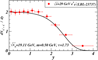
Figure 1: (Color online) The rapidity distribution of pions in high-energy $e^{+}$-$e^{-}$ annihilation at $\sqrt{s}=$29 GeV, out of which $\sqrt{s_{\pi}}$=19.11 GeV goes into producing pions. The data is from Aih88 ; Hof88 ; Aihnote and the solid curve is from Eq. (82) with $m=0.50$ GeV, $\nu=1.73$.

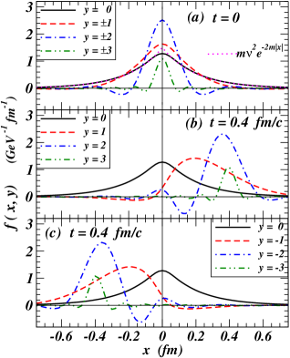
Figure 2: (Color online) Wigner function $f(x,y)$ as a function of $x$ for different values of positive $y$. Fig. 2(a) gives $f(x,y)$ for $t=0$, and the dotted curve is the approximate analytical result for $f(x,y=0)$ at $t=0$ given by Eq. (86). Fig. 2(b) gives $f(x,y)$ for positive $y$ at $t=0.4$ fm/c, and Fig. 2(c) for negative $y$ at $t=0.4$ fm/c.

It is of interest to study a specific numerical example to illustrate the space-time dynamics of string fragmentation. We can consider the experimental rapidity distribution of charged pions in $e^{+}$-$e^{-}$ annihilation at $\sqrt{s}=29$ GeV Aih88 ; Hof88 . In such an annihilation, heavier particles such as kaons and baryons are also produced and they carry a fraction of the initial energy. By integrating out the experimental $dN/dyp_{t}dp_{t}$ data in Table 11 of Ref. Aih88 , the particle multiplicities of the produced pions, kaons, and baryons are in the ratio of $N_{\pi}:N_{K}:N_{N}=80:15:5$ and the total energies of the produced particles are 19.11, 7.10, and 2.53 GeV for pions, kaons, and nucleons respectively Aih88 .

Rather than attempting to model the production of heavier mesons here, we shall instead simply consider pions only and study an idealized situation in which the system fragments only into pions. We can consider the pions to take up $\sqrt{s_{\pi}}=$19.11 GeV of the total energy and fit the rapidity distribution of the pions with Eqs. (82) and (83) which contain only two unknown parameters: the mass $m$ and the effective charge $\nu$. The pions have an average transverse momentum of 0.48 GeV Aih88 , which corresponds to a pion transverse mass of $m_{\pi{}_{T}}=\sqrt{p_{T}^{2}+m_{\pi}^{2}}=0.50$ GeV. In approximately compactifying QCD4 to QCD2 and QED2, we have subsumed the details of the transverse degree of freedom by using the transverse mass of quarks. With the quark mass modified to be the transverse quark mass by this compactification, the corresponding produced boson mass should also be modified to be the transverse boson mass of the observed boson. Accordingly, the boson mass $m$ of the produced particle in Eqs. (83) should be taken to be the pion transverse mass of $m=m_{\pi{}_{T}}=0.50$ GeV. The theoretical rapidity distribution of charged pions can then be calculated with Eq. (82) with the effective charge $\nu$ as the only unknown parameter. The effective charge value of $\nu=\sqrt{3}$ Won91 gives a good description of the experimental rapidity plateau of the produced pions Aih88 ; Hof88 ; Aihnote , as shown in Fig. 1. It is interesting that as $N_{f}$ is related to $\nu$ by $N_{f}=\nu^{2}$. It appears phenomenologically that the effective number of flavors participating in the excitation of the vacuum for $e^{+}$-$e^{-}$ annihilation at this energy is 3. This effective charge is in line with the discussions in in Section III, where the strengths of the underlying color source generating the excitation of the gauge fields is proportional linearly to the number of flavors $N_{f}$.

From Eq. (81), the width parameter of the initial charge current $\sigma$ is 0.33/GeV or 0.065 fm, which is a narrow current distribution. With the knowledge of $\sigma$ and $\nu$, the Fourier coefficient $c(p^{1})$ can be evaluated the Wigner function from Eq. (71) by direct numerical integration. Fig. 2 shows the Wigner function $f(x,y)$ as a function of $x$, for various values of $y$ at $t=$0 in Fig. 2(a), for positive $y$ at $t=$0.4 fm/c in Fig. 2(b), and for negative $y$ at $t=$0.4 fm/c in Fig. 2(c). The range of rapidities in Fig. (1) span over different regions of the rapidity plateau as one can see in Fig. 1. One notes the following interesting features.

1. At $t$=0, the peak of all Wigner functions occur at $x=0$, indicating that all produced bosons with different momenta in different regions of the rapidity plateau are present at $t=0$. This picture is in contrast to the momentum-space-time ordering of the classical picture of particle production where particles of larger momenta $|y|$ are produced at larger $|x|$ at a later time.

2. The Wigner function is symmetrical with respect to the changes of both $x$ to $-x$ and $y$ to $-y$. That is, $f(x,y;t)=f(-x,-y;t)$.

3. The Wigner function for the zero-mode with $y=0$ behaves approximately as $\nu^{2}e^{-2m|x|}$ (see Eq. (86) below) and is positive definite. The width of the dominant Wigner function peak for $|y|\neq 0$ decreases as a function of increasing $|y|$, as expected from the uncertainty principle.

4. Except for Wigner function of the zero-mode with $y=0$ which is positive definite, the Wigner function of other longitudinal momenta oscillates as a function of space and time and can assume negative values at locations away from the dominant peaks.

5. Except for Wigner function of the zero-mode with $y=0$ which does not depend on time, the dominant peaks of the Wigner function moves to the positive longitudinal direction for positive $y$ and to the negative longitudinal direction for negative $y$. The speed of the movement of the peak position increases with an increasing magnitude of the longitudinal momentum.

From the above features, one can readily understand the movement of the peak positions of the Wigner functions for different $y$ values, as they follow the motion of what is expected from classical physics.

How do we understand the relatively large width of the spatial distribution of the Wigner function of the zero-mode with $y=0$? The half width of the distribution is about 0.2 fm, which is large compared to the width parameter $\sigma\sim$ 0.065 fm for the charge current. What physical quantity determines the scale of this width? It is instructive to check the Wigner function for this zero mode case. For $y=0$, the Wigner function becomes

$$f(x,y=0) = \frac{1}{2\pi}\int_{0}^{\infty}dq\,\cos(qx)\frac{m^{2}}{(q^{2}/4)+m^{2}}2\nu^{2}\frac{(q\pi\sigma/4)^{2}}{\sinh^{2}(q\pi\sigma/4)},$$ (85)

$$\sim \frac{\nu^{2}}{\pi}\int_{0}^{\infty}dq\,\cos(qx)\frac{m^{2}}{(q^{2}/4)+m^{2}}\Theta(\Omega-|q|),$$

where $\Omega\sim 2\xi_{0}/\pi\sigma=2\times 1.491/\pi\sigma$. In the spatial region where $\Omega x\gg 1$, we have

$$f(x,y=0) \sim \frac{4xm^{2}\nu^{2}}{\pi}\int_{0}^{\Omega x}d\xi\,\frac{\cos\xi}{{\xi^{2}+4m^{2}x^{2}}},$$ (86)

$$\sim m\nu^{2}e^{-2m|x|}.$$

We plot the function $m\nu^{2}e^{-2m|x|}$ as the dotted curve in Fig. 2(a). We find that except in the region of $x\lesssim 0.05$ fm, it agrees with the exact Wigner function $f(x,y=0)$. It is also independent of $t$, as $p^{0}-{p^{0}}^{\prime}=0$ for $k=0$ in Eq. (71). The analytical result shows that the width of Wigner function for the zero mode with $y=0$ is governed by the mass boson mass as (width)$\sim\hbar/m$.

How do we understand the origin of the large range of momentum $y$ values that are present in the Wigner function at $t=0$? From our derivation of the Wigner function, we note that the presence of an initial charge current with a very narrow width in $j^{\mu}(x,t)$ leads to a wave packet of the boson field $\phi$ in Eq. (52), as a coherent sum of a large number of waves of different momentum components $p^{1}$. The greater the energy of the fragmenting string, the narrower is the initial spatial current $j^{\mu}(x,t)$, and the greater will be the spread of the momentum components of the boson wave packet $\phi(x,t)$, as indicated by the large width of $|c(p^{1})|$. The coherent sum of the boson field gives rise to the corresponding Wigner function that depends on the correlation between the Fourier components at different momenta. The Wigner function has a spatial extension much greater than that of the initial charge current.

In physical terms, there are two peculiar quantum effects that make QED2 different from those from classical considerations of string fragmentation. Firstly, the produced bosons occur initially in a spatial region more extended than the width of the initial fermion current. They are governed more by the produced boson mass and the uncertainty principle than by the spatial width of the initial current. Secondly, produced particles of different momenta emerge at the initial moment of string fragmentation. These peculiarities does not violate causality because the dynamics of string fragmentation in QED2 is not just a two-body problem involving only the fragmenting valence fermion and antifermion. It involves a many-body problem of particles, antiparticles, and gauge fields interacting self-consistently with particles in the Dirac sea over an extended region of space and time, giving rise to the excitations of the vacuum which manifests themselves as quanta of the massive boson field Sch62 ; Ili84 ; Won94 .

VII Interference in the fragmentation of many identical strings

The process of string fragmentation is a quantum phenomenon. We therefore expects effects of quantum interference when many identical strings fragment. As a well-defined interference phenomenon, it possesses its own intrinsic theoretical interest. Furthermore, the presence or absence of the characteristics of interference may be used to provide useful information on the fragmenting strings concerning their properties of being identical or non-identical, when they occur in close vicinity of each others.

We consider the occurrence of $n$ identical strings at longitudinal locations $\chi_{i}$ centered around the longitudinal origin, in the center-of-mass frame. For simplicity, we shall take the fragmentation to be occurring at the same time and that the strings are identical in their characteristics. In this case, the fragmentation can be idealized as $n$ interacting fermion-antifermion pairs. In each pair, the fermion and the antifermion pulls apart in opposite directions. The time-like fermion current $j^{0}(x,0)=0$ is initially zero at all spatial points and the initial space-like current $j^{1}(x,0)$ pulls each fermion-antifermion pair away from each other.

In representing the sum of the fermion currents in a many-string system, we would like to introduce the concept of the sense $\zeta$ of a fragmenting string. Consider the fragmentation of a string starting with a fermion and an antifermion locating at a spatial point. The sense of a string specifies the direction of motion of the fermion, with the antifermion traveling in the opposite direction. We choose the convention that the sense $\zeta$ is equal to 1 when the fermion travels to the positive longitudinal direction and $\zeta$ is -1 when the fermion travels to the negative longitudinal direction. The sense of motion clearly is immaterial for a single string. However, they are important in the fragmentation of a many-string system, as we shall see.

The total current $j_{\rm tot}^{\mu}(x,t)$ from the $n$ fermion-antifermion pairs can be described as

$$j_{\rm tot}^{0}(x,t)=\frac{e\nu}{2\sigma}\sum_{i=1}^{n}\zeta_{i}\left(\frac{1}{\cosh^{2}\left(\frac{x-\chi_{i}+t}{\sigma}\right)}-\frac{1}{\cosh^{2}\left(\frac{x-\chi_{i}-t}{\sigma}\right)}\right),$$ (87)

and

$$j_{\rm tot}^{1}(x,t)=\frac{e\nu}{2\sigma}\sum_{i=1}^{n}\zeta_{i}\left(\frac{1}{\cosh^{2}\left(\frac{x-\chi_{i}+t}{\sigma}\right)}+\frac{1}{\cosh^{2}\left(\frac{x-\chi_{i}-t}{\sigma}\right)}\right),$$ (88)

where the width parameter $\sigma$ will need to be self-consistently determined in terms of the total energy $\sqrt{s}$ of the $n$-string system because the strings will interfere with each other in generating the particle rapidity spectrum.

The Fourier transform of the initial current can be easily obtained and they are related to ${\tilde{j}}^{\mu}(p^{1})$ of Eqs. (78) and (79) by

$${\tilde{j}}_{\rm tot}^{\mu}(p^{1})=\sum_{i=1}^{n}\zeta_{i}e^{-ip^{1}\chi_{i}}{\tilde{j^{\mu}}}(p^{1}).$$ (89)

Similarly, the total Fourier component for Eq. (55) is

$$c_{\rm tot}(p^{1})=\sum_{i=1}^{n}\zeta_{i}e^{-ip^{1}\chi_{i}}c(p^{1}),$$ (90)

where $c(p^{1})$ is given by Eq. (55). As a consequence, Eq. (64) for the momentum distribution of produced particles is modified to be

$$\frac{dN_{\rm tot}}{dp^{1}} = \frac{c_{\rm tot}(p^{1})c_{\rm tot}^{*}(p^{1})}{2p^{0}}$$ (91)

$$= \left[n+\sum_{i>j}^{n}2\zeta_{i}\zeta_{j}\cos\{p^{1}(\chi_{i}-\chi_{j})\}\right]\frac{c(p^{1})c^{*}(p^{1})}{2p^{0}}.$$

The rapidity distribution for the fragmentation of $n$ strings is

$$\frac{dN_{\rm tot}}{dy}=\left[n+\sum_{i>j}^{n}2\zeta_{i}\zeta_{j}\cos\{(m\,\sinh y)(\chi_{i}-\chi_{j})\}\right]\frac{c(p^{1})c^{*}(p^{1})}{2}.$$ (92)

For the Fourier coefficient given by Eqs. (80), we obtain

$$\frac{dN_{\rm tot}}{dy}=\left[n+\sum_{i>j}^{n}2\zeta_{i}\zeta_{j}\cos\{(m\,\sinh y\,)(\chi_{i}-\chi_{j})\}\right]\frac{\nu^{2}\xi^{2}}{\sinh^{2}\xi},$$ (93)

where $\xi={\nu^{2}\pi^{2}m\sinh y}/{3\sqrt{s}}$ is given by Eq. (83). This equation can also be written as

$$\frac{dN_{\rm tot}}{dy}=\left[n+\sum_{i>j}^{n}2\zeta_{i}\zeta_{j}\cos\{(m\,\sinh y)\,(\chi_{i}-\chi_{j})\}\right]\frac{dN_{\rm single}}{dy},$$ (94)

where $dN_{\rm single}/dy=\nu^{2}{\xi^{2}}/{\sinh^{2}\xi}$. The total energy of the $n$-string system is given by

$$\sqrt{s}=\int dy\,m\,\zeta_{i}\zeta_{j}\cosh y\,\left[n+\sum_{i>j}^{n}2\zeta_{i}\zeta_{j}\cos\{(m\,\sinh y)\,(\chi_{i}-\chi_{j})\}\right]\frac{\nu^{2}\xi^{2}}{\sinh^{2}\xi},$$ (95)

which provides a relation between $\sqrt{s}$ and $\sigma$.

The Wigner function for the fragmentation of $n$ strings is now modified to be

$$f_{\rm tot}(x,k) = \frac{1}{4\pi k^{0}}\int dqe^{iq[x-(p^{0}(q)-{p^{0}}^{\prime}(q))t]}\frac{p^{0}{p^{0}}^{\prime}+(k^{0})^{2}-q^{2}/4}{2p^{0}{{p^{0}}^{\prime}}}$$ (96)

$$\times \sum_{i,j=1}^{n}\zeta_{i}\zeta_{j}e^{-i(k+q/2)\chi_{i}+i(k-q/2)\chi_{j}}c(k+\frac{q}{2})c^{*}(k-\frac{q}{2}).$$

We can simplify the above expression by noting that

$$e^{iqx}e^{-i(k+q/2)\chi_{i}+i(k-q/2)\chi_{j}}=e^{iq(x-{\bar{\chi}}_{ij})-ik(\chi_{i}-\chi_{j})},$$ (97)

where ${\bar{\chi}}_{ij}$ is the average of the initial longitudinal positions of strings $i$ and $j$,

$${\bar{\chi}}_{ij}=(\chi_{i}+\chi_{j})/2.$$ (98)

Therefore, we get

$$\sum_{i,j=1}^{n}\zeta_{i}\zeta_{j}e^{iqx}e^{-i(k+q/2)\chi_{i}+i(k-q/2)\chi_{j}}=\sum_{i}^{n}e^{iq(x-{\chi}_{i})}+\sum_{i>j}^{n}\zeta_{i}\zeta_{j}e^{iq(x-{\bar{\chi}}_{ij})}2\zeta_{i}\zeta_{j}\cos\{k(\chi_{i}-\chi_{j})\}.$$ (99)

We can thus write the total Wigner function of the produced particles in the fragmentation of $n$ strings as

$$f_{\rm tot}(x,k)=\sum_{i=1}^{n}f_{\rm single}(x-\chi_{i},k)+\sum_{i>j}^{n}2\zeta_{i}\zeta_{j}\cos\{k(\chi_{i}-\chi_{j})\}f_{\rm single}(x-{\bar{\chi}}_{ij},k).$$ (100)

The corresponding Wigner function $f_{\rm tot}(x,y)$ can then be obtained as $f_{\rm tot}(x,y)=k^{0}f_{\rm tot}(x,k)$ evaluated at $k=m\sinh(y)$.

We note from these results that there are important interference effects between identical strings. The interference appears in the form of a cosine function $\zeta_{i}\zeta_{j}\cos\{k(\chi_{i}-\chi_{j})\}$ that depends on the momentum of the produced particle, the initial spatial separation between the strings, and the senses of the strings. The dependence on the string separation is similar to the interference in the emission of particles from different sources in intensity interferometry Won04 .

In the case when the strings are far apart such that $|\chi_{i}-\chi_{j}|$ is large, the cross terms in the Wigner function with $i\neq j$ in Eq. (100) oscillate rapidly about zero (for non-zero modes). The cross terms will provide only small average contributions and the direct terms dominate. In that case when strings are far apart, $f_{\rm tot}(x,k)\approx\sum_{i}^{n}f_{\rm single}(x-\chi_{i},k)$ for $|k|\neq 0$, which is the sum of independent Wigner functions for separated strings.

In the other extreme, all strings are located at the same spatial point. Among these $n$ strings, there are $n_{+}$ strings with the $\zeta=1$ sense and $n_{-}=n-n_{+}$ strings with the opposite sense, $\zeta=-1$. Then, when all the strings occur at the same point, we have

$$dN_{\rm tot}/dy=(n_{+}-n_{-})^{2}dN_{\rm single}/dy,$$ (101)

and

$$f_{\rm tot}(x,k{\rm~{}or~{}}y)=(n_{+}-n_{-})^{2}f_{\rm single}(x,k{\rm~{}or~{}}y).$$ (102)

If all the strings are aligned in the same direction then $dN_{\rm tot}/dy=n^{2}dN_{\rm single}/dy$. On the other hand, if $n_{+}=n_{-}$, then $dN_{\rm single}/dy=0$ and $f_{\rm tot}(x,y)=0$. In general, the greater the difference $|n_{+}-n_{-}|$, the larger is $dN_{\rm tot}/dy$ and $f_{\rm tot}(x,y)$. The strength of the Wigner function of one string of one sense is canceled by the Wigner function of the string of the opposite sense. This cancellation of the string strength cannot be complete if the number of strings is odd.

VIII Wigner function in the fragmentation of identical strings

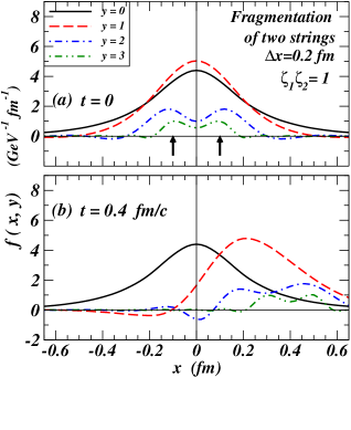
Figure 3: (Color online) The Wigner function $f(x,y)$ for two strings with the same sense, $\zeta_{1}\zeta_{2}=1$. The strings are initially located at $x=-0.1$ and $x=0.1$ fm indicated by the two arrows, with a separation of $\Delta x=0.2$ fm. Fig. 3(a) is for $t=0$ and Fig. 3(b) is for $t=0.4$ fm/c.

As an example, it is instructive to evaluate the Wigner function for a few cases to see its dependence on the separation between the strings and their relative sense of directions. We show the time variation of the Wigner function for two strings each of which, if separated, has characteristics the same as those in Fig. 2. We examine first the case of two identical strings with the same sense so that $\zeta_{1}\zeta_{2}=1$. In Fig. 3, the origins of these two strings are initially located at $\chi_{1}=-0.1$ and $\chi_{2}=0.1$ fm with a separation $\Delta x=0.2$ fm. In Fig. 4, they are located at $\chi_{1}=-0.04$ and $\chi_{2}=0.04$ fm with a separation $\Delta x=0.08$ fm. The locations of the origins of the strings are indicated by two thick arrows in Figs. 3 and 4.

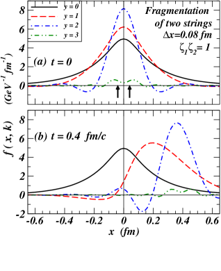
Figure 4: (Color online) Wigner function $f(x,y)$ as a function of $x$ for different values of $y$ for two strings located at $x=-0.04$ and $x=0.04$ fm, as indicated by the two arrows, with a separation of $\Delta x=0.08$ fm. Fig. 4(a) is for $t=0$ and Fig. 4(b) is for $t=0.4$ fm/c.

We note the following features from the dynamics of the Wigner function from Figs. 3 and 4.

1. Similar to the case of a single string, all bosons of different momenta in different regions of the rapidity plateau are present at $t=0$. This picture is in contrast to the momentum-space-time ordering of the classical picture of particle production.

2. The magnitude and the width of Wigner function of the zero-mode with $y=0$ are quite large when $\zeta_{1}\zeta_{2}=1$. The magnitude of the peak is about three times that of Fig. 2. For this case of two strings, there are three contributions, corresponding to two contributions centered at the origins of the strings, plus an additional contribution at $x=0$, as given by Eq. (100). For the $y$=0 zero mode, all these three pieces merge together to form a broad peak at $x=0$ that is independent of time.

3. For the low rapidity case with $y=1$, the different contributions to the Wigner function merge into a single peak for both separations of $\Delta x=0.2$ and 0.08 fm.

4. For higher rapidities with $y\geq 2$, the different contributions to the Wigner function merge into a single peak for the case of $\Delta=0.08$ fm, but splits into two peaks for $\Delta x=0.2$ fm. This shows that the Wigner functions for many strings tend to merge together into a single structure, when the separation between strings is small.

5. As a function of time, the peaks of the Wigner function move in the positive $x$ direction for positive values of $y$. They move to the negative $x$ direction for negative values of $y$. The low-momentum Wigner functions with $y=1$ remain to be merged as they propagate. For the case of $y\geq 2$ and $\Delta x=0.2$ fm, there appear two propagating peaks corresponding to the propagation of the produced particles from the two different strings. For the case $y\geq 2$ and $\Delta x=0.08$ fm, the Wigner functions from the two strings remain merged during their propagation.

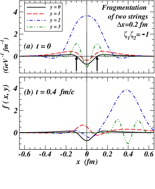
Figure 5: (Color online) The Wigner function $f(x,y)$ as a function of $x$ for different values of $y$ for two strings with opposite senses, $\zeta_{1}\zeta_{2}=-1$. The strings are initially located at $x=-0.1$ and $x=0.1$ fm indicated by the two arrows, with a separation of $\Delta x=0.2$ fm. Fig. 5(a) is for $t=0$ and Fig. 5(b) is for $t=0.4$ fm/c.

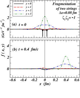
Figure 6: (Color online) The Wigner function $f(x,y)$ as a function of $x$ for different values of $y$ for two strings with opposite senses, $\zeta_{1}\zeta_{2}=-1$. The strings are initially located at $x=-0.04$ and $x=0.04$ fm indicated by the two arrows, with a separation of $\Delta x=0.08$ fm. Fig. 8(a) is for $t=0$ and Fig. 8(b) is for $t=0.4$ fm/c.

It is instructive to evaluate next the Wigner function for the case of two identical strings with the opposite sense so that $\zeta_{1}\zeta_{2}=-1$. We consider again two strings each of which, if separated, has characteristics same as those in Fig. 2. In Fig. 5, these two strings are initially located at $\chi_{1}=-0.1$ and $\chi_{2}=0.1$ fm with a separation $\Delta x=0.2$ fm. In Fig. 6, they are located at $\chi_{1}=-0.04$ and $\chi_{2}=0.04$ fm, with a separation $\Delta x=0.08$ fm. The positions of the origins of the strings are indicated by the two thick arrows in Figs. 5 and 6.

The results in Figs. 5 and 6 show that in the fragmentation of two strings with opposite senses, the magnitude of the Wigner function is much reduced from the fragmentation of two strings with the same sense. The zero-mode Wigner function is negative at $x=0$, in contrast to the positive definite property of the Wigner function for a single string or for two strings with the same sense. There are oscillations of the Wigner function for different momenta at $t=0$. For $t>0$, the dominant peaks of the Wigner function propagate according to their momenta.

As the separation between the strings becomes smaller, the Wigner function of opposite senses tend to cancel and the magnitude of the Wigner function decreases, as shown in Fig. 6. As we remarked earlier, the Wigner function is reduced to zero in the limit when the two identical strings with opposite senses coincide.

IX Dynamics of the Wigner function in the fragmentation of independent strings

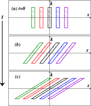
Figure 7: (Color online) Schematic space-time evolution of the Wigner function $f(x,y)$ of produced particles from many independent strings. Fig. 7(a) is for $t=0$, 7(b) and 7(c) are the schematic configurations at subsequent times.

The last two sections deal with the fragmentation of identical strings for which interference effects are present. In a nucleus-nucleus collision, the number of nucleon-nucleon collisions is large in a local neighborhood. We expect that each nucleon-nucleon collision produces at least two strings spanned between the quark of one nucleon and the diquark of the other nucleon. The types of strings that are formed are however very large in numbers as each string will be characterized by the color and the flavor of the quark and the diquark at its two ends, and by the color gauge field component $a$ of $A^{\nu a}$ the string can excite. As a consequence, the probability of a neighboring string to be identical is of order $1/[N_{c}^{2}N_{f}({\rm q})N_{f}({\rm qq})(N_{c}^{2}-1)]$ which is quite small. The production process in string fragmentation in a nucleus-nucleus collision is likely to involve the fragmentation of independent non-identical strings. It is appropriate to examine the space-time dynamics of produced particles in the fragmentation of many independent strings.

In a nucleus-nucleus collision in the center-of-mass system, the average longitudinal separation between neighboring strings is $d/\gamma$ where $d\sim 1.9$ fm is the average nucleon-nucleon separation for a nucleus at rest and $\gamma=\sqrt{s_{{}_{NN}}}/m_{N}$ is the Lorentz contraction factor. On the other hand, the width of the Wigner function for the zero mode with $y$=0 is of order $\hbar/m_{\pi T}$, as indicated by Eq. (86) . Whether the Wigner function will be separated or will overlap depend on whether $d/\gamma$ is greater or less than $\hbar/m_{\pi T}$:

$$\begin{cases}{\rm If~{}~{}}d/\gamma&\gtrsim~{}~{}~{}\hbar/m_{\pi T},{\rm~{}~{}~{}strings~{}are~{}separated.}\\ {\rm If~{}~{}}d/\gamma&\lesssim~{}~{}~{}\hbar/m_{\pi T},{\rm~{}~{}~{}strings~{}overlap.}\end{cases}$$ (104)

As the pion transverse mass $m_{\pi T}$ is of order 0.5 GeV, the Wigner functions will be separated from each other if the collision energy per nucleon in the center-of-mass system is $\sqrt{s_{{}_{NN}}}\lesssim 5$ GeV and will overlap each other if $\sqrt{s_{{}_{NN}}}\gtrsim 5$ GeV.

For each string, particles of different rapidities in different regions of the rapidity plateau are produced at the moment of string fragmentation. They propagate toward opposite longitudinal directions according to their rapidities. We can depict the dynamics of the density of Wigner functions as those of one of the rectangular regions in Fig. 7.

How the partons evolve after production in a heavy-ion collision at high energies is a complex problem which will require extensive future investigations. Our experience with the phase space dynamics of nucleons in nucleus-nucleus collisions as investigated earlier in Won82a ; Won82 may furnish an approximate guide to speculate on the behavior of partons in high energy nuclear collisions.

We can discuss first the case of $\sqrt{s_{{}_{NN}}}\lesssim 5$ GeV in the fragmentation of independent and separated strings as shown in Fig. 7. Produced particles in these separated strings will stream from one point to another point as time proceeds. Their streaming will lead to three important effects. First, they will replenish those particles that have just streamed away from the point of production, as is depicted in Fig. 7(b) and 7(c). Secondly, as a result of their streaming, they will encounter at the same longitudinal point produced particles streaming from neighboring points in the opposite direction. Such encountering will lead to collisions. The discussion of the collisions of the produced particles necessitates the inclusion of the transverse degrees of freedom. It is necessary to restore the transverse momentum distribution of the produced particles by using information on the transverse eigenfunctions of the quarks and antiquarks. These collision of produced particle will convert longitudinal momenta to transverse momenta, leading to medium particles with smaller longitudinal momenta but greater transverse momenta in the approach to equilibrium. Thirdly, the produced particles will likely be subject to strong residual interactions after production. The interaction is stronger, the more the strings are closer packed together at higher collision energies. Fourthly, because of their mutual interaction and the nature of color confinement, those produced particles reaching the boundary region will form a surface in the boundary region, against which produced particle arriving later will collide. Part of these particles will continue to propagate forward as a result of the collision with the longitudinal boundary and will stretch the surface to a greater longitudinal extension. However, part of the colliding produced particles will be reflected from the surface and will stream in the backward direction, replenishing some of the partons that have streamed backward, similar to the description in Fig. 1 of Won82 , in the approach to equilibrium.

We consider next the heavy-ion collisions at very high energies. For a collision energy of 100 GeV per nucleon at RHIC, the average longitudinal separation between strings is of order 0.019 fm which is much smaller than the width of the Wigner function, $\hbar/m_{\pi T}$. The nucleus-nucleus collision leads to a large overlap of the fragmenting strings. Because of the strong overlap of the strings, the produced quanta will propagate to the longitudinal boundary together in nearly the same speed and nearly in unison. Because of the strong overlap and the Lorentz contraction, there is a large density and large interaction among produced particles after they are produced. The produced particles will propagate according to their longitudinal rapidities. Partons with large rapidities will reach the boundary first, forming a surface region. The interacting partons near the surface will collide with the confining and moving surface. As a result of the collision with the boundary, part of these partons will continue forward, and they will stretch the surface boundary to a greater longitudinal extension to keep it a continuously moving boundary. Because of the confining interactions at the moving boundary, some of the other partons will come to the classical turning point at the moving boundary. They will then be reflected from the surface and will flow in the backward direction. The reflection of confining partons leads to two important effects. First, the reflected partons will replenish some of the partons that have streamed backward, as depicted in Fig. 1 of Ref. Won82 . Secondly, the reflected partons will encounter partons streaming in the opposite direction. Such encountering will lead to collisions which will convert longitudinal momentum to transverse momentum, leading to medium particles with a smaller average longitudinal momentum. The collisions may relax the rapidity distribution from an initial rapidity plateau Yan08 to a Gaussian rapidity distribution at the end of nucleus-nucleus collision Mur04 ; Ste05 ; Ste07 . Whether or not such a scenario indeed occurs will require more future analyses.

X Discussion and Conclusions

We investigate the space-time behavior of produced particles in the fragmentation of a string in QED2. We obtain a relation between the rapidity distribution and the Fourier transforms of the initial fermion current. We find that the rapidity plateau at high energies arises as a consequence of a localized initial fermion current. The Wigner function of the produced particles show that particles with momenta in different regions of the rapidity plateau are present at the moment of string fragmentation, with the width of their spatial distributions decreasing with an increasing center-of-mass energy. The Wigner function exhibits the effects of interference in the fragmentation of many identical strings.

Because QED2 mimics many features of QCD4, it is useful to examine the circumstances in which a QCD4 systems can be approximated by QED2. We show first how QCD4 with transverse confinement can be approximately compactified as QCD2 with a transverse quark mass $m_{{}_{T}}$ obtained by solving a set of coupled transverse eigenvalue equations. Furthermore, in the limit of the strong coupling and the large number of flavors $N_{f}$, QCD2 admits Schwinger QED2-type solutions. It is for these reasons that QED2 can mimic many important features of QCD4, including the properties of the proper high-energy rapidity plateau behavior, quark confinement, charge screening, and chiral symmetry breaking. In the absence of rigorous non-perturbative QCD4 solutions, it is therefore reasonable to study the particle production process phenomenologically using Schwinger’s QED2 model, with the boson quanta of QED2 considered as analogous to the boson quanta in QCD.

There are however important differences which must be kept in mind in the discussion of the dynamics subsequent to the fragmentation of strings. Free bosons are the quanta of QED2 while strongly interacting gluons and quarks and relatively weakly interacting hadrons are quanta of QCD4 at different temperatures of the QCD system. In a nucleus-nucleus collision at high energies, the particles produced after the fragmentation the strings will be subject to strong interactions with the dense medium of produced particles in their vicinity after production. These interactions are important as the strings overlap strongly owing to the Lorentz contraction. The large number of colors and flavors make it likely that the overlapping strings are of different types and do not interfere. As a consequence, the density of the produced particles accumulatively increases as the density of strings increases. It will be necessary to include these strong interactions between the produced particles in order to describe better the subsequent dynamics. It will also be necessary to restore the transverse degrees of freedom for a better description by using information on the transverse eigenfunctions of the quarks and antiquarks and their transverse momentum distributions. Our formulation of the approximate compactification between transversely-confined QCD4 into QCD2 facilitates such a restoration.

The main feature inferred from our present analysis is that in a string fragmentation, boson field quanta with momenta in different regions of the rapidity plateau are present in the initial Wigner function at the moment of string fragmentation. This peculiar behavior arises from the quantum effects of the vacuum structure. Particles in the vacuum of the Dirac sea participate in the interaction as the valence fermions, antifermions, and gauge fields change with space and time. The non-perturbative self-consistent response of particles in the Dirac sea leads to the production of boson quanta with momenta in different regions of the rapidity plateau at the moment of string fragmentation, in contrast to the classical picture of string fragmentation where there is a momentum-space-time ordering of produced particles.

Our analysis of the dynamics of the Wigner function places it in the class of initial-state-interaction description of quantum chromodynamics. Our result that partons in different regions of rapidities over the rapidity plateau are produced at the moment of collision is in line with many other well-justified initial-state-interaction models, such as the parton model Fey69 , the Drell-Yan process Dre71 , the multi-peripheral model Che68 , and the dipole approach of photon-induced strong interactions Huf00 . These are models in which the constituent particles or produced particles are present at or before the collision process at $t=0$.

With regard to the momentum kick model which motivated the present analysis, the above results may resolve one of the puzzles concerning the possible occurrence of the particles with large longitudinal momenta in the early stage of the nucleus-nucleus collisions. Partons of different rapidities are present in the initial parton momentum distribution at fragmentation. The jet produced in one of the nucleon-nucleon collisions can find partons of large rapidities in the early environment. There can be collisions between the jet and these high-rapidity partons, which show up as ridge particles in coincidence with the jet. Just as the presence of antiquark partons from the quark-antiquark sea is revealed by the occurrence of the Drell-Yan process in the initial-state-interaction picture, so it is here that the presence of the rapidity plateau in the early parton momentum distribution is revealed by the occurrence of large rapidity associated particles in coincidence with the near-side jet in the PHOBOS experiments.

Acknowledgment

The authors would like to thank Profs. H. W. Crater and Che-Ming Ko for helpful discussions. This research was supported in part by the Division of Nuclear Physics, U.S. Department of Energy, under Contract No. DE-AC05-00OR22725, managed by UT-Battelle, LLC.

References

- (1) S. Wolfram, Proc. 15th Recontre de Moriond (1980), ed. by Tran Thanh Van; G. C. Fox and S. Wolfram, Nucl. Phys. 238, 492 (1984).
- (2) L. Van Hove, A. Giovannini, Acta Phys. Polon. B19, 931 (1988); M. Garetto, A. Giovannini, T. Sjostrand, L. van Hove, CERN Report CERN-TH-5252/88, Presented at Perugia Workshop on Multiparticle Dynamics, Perugia, Italy, Jun 21-28, 1988; Y. L. Dokshizer, V. A. Khoze, S. I. Troyan, in Perturbative Quantum Chromodynamics, Ed. by A. H. Mueller, World Publishing, Singapore 1989, p. 241.
- (3) R. O’dorico, Nucl. Phys. B172, 157 (1980); R. O’dorico, Comp. Phys. Comm. 32, 139 (1984); G. Marchesini and B. R. Webber, Nucl. Phys. B238, 1 (1984); B. R. Webber, Nucl. Phys. B238, 492 (1984); T. D. Gottschalk, Nucl. Phys. B239, 325 (1984).
- (4) B. Andersson, G. Gustafson, and T. Sjöstrand, Zeit. für Phys. C20, 317 (1983); B. Andersson, G. Gustafson, G. Ingelman, and T. Sjöstrand, Phys. Rep. 97, 31 (1983); T. Sjöstrand and M. Bengtsson, Computer Physics Comm. 43, 367 (1987); B. Andersson, G. Gustavson, and B. Nilsson-Alqvist, Nucl. Phys. B281, 289 (1987).
- (5) A. Capella and A. Krzywicki, Phys. Rev. D18, 3357 (1978); A. Capella and J. Tran Thanh Van, Zeit. für Phys. C10, 249 (1981); A. Capella , Zeit. für Phys. C33, 541 (1987); A. Capella and J. Tran Thanh Van, Zeit. Phys. C38, 177 (1988); N. Armesto and C. Pajares, Int. J. Mod. Physi A15, 2019 (2000).
- (6) K. Werner, Phys. Rev. D39, 780 (1988).
- (7) H. Sorge, H. Stöcker, and W. Greiner, Nucl. Phys. A498, 567c (1989);
- (8) C. Y. Wong, and Z. D. Lu, Phsy. Rev. D39, 2606 (1989).
- (9) X. N. Wang and M. Gyulassy, Comp. Phys. Comm. 83, 307 (1994).
- (10) K. Geiger and B. Müller, Nucl. Phys. A544, 467c (1992);
- (11) L. D. McLerran and R. Venugopalan, Phys. Rev. D49, 2233 (1994); L. D. McLerran and R. Venugopalan, Phys. Rev. D49, 3352 (1994); L. D. McLerran and R. Venugopalan, Phys. Rev. D50, 2225 (1994). A. Kovner, L. McLerran, and H. Weigert, Phsy. Rev. D52, 6231 (1995).
- (12) Zi-Wei Lin, Che Ming Ko, Bao-An Li and Bin Zhang, and Subrata Pal, Phy. Rev. C72, 064901 (2005).
- (13) S. Jeon and J. Kapusta, Phsy. Rev. C56, 468 (1997).
- (14) J. Schwinger, Phys. Rev. 128, 2425 (1962); J. Schwinger, in , Trieste Lectures, 1962 (I.A.E.A., Vienna, 1963), p. 89.
- (15) J. H. Lowenstein and J. A. Swieca, Ann. Phys. (N.Y.) 68, 172 (1971).
- (16) S. Coleman, R. Jackiw, and L. Susskind, Ann. Phys. 93, 267 (1975).
- (17) S. Coleman, Ann. Phys. 101, 239 (1976).
- (18) A. Casher, J. Kogut, and L. Susskind, Phys. Rev. D10, 732 (1974).
- (19) J. D. Bjorken, Phys. Rev. D 27, 140 (1983).
- (20) N. P. Ilieva and V. N. Pervushin, Sov. J. Nucl. Phys. 39, 638 (1984).
- (21) T. Eller, H-C. Pauli, and S. Brodsky, Phys. Rev. D35, 1493 (1987); T. Eller and H-C. Pauli, Zeit. für Phys. 42, 59 (1989).
- (22) T. Fujita and J. Hüfner, Phys. Rev. D40, 604, (1989).
- (23) C. Y. Wong, R. C. Wang, and C. C. Shih, Phys. Rev. D 44, 257 (1991).
- (24) C. Y. Wong, Introduction to High-Energy Heavy-Ion Collisions, World Scientific Publisher, 1994.
- (25) H. Aihara (TPC/Two_Gamma Collaboration), Lawrence Berkeley Laboratory Report LBL-23737 (1988).
- (26) W. Hofmann, Ann. Rev. Nucl. Sci. 38, 279 (1988).
- (27) Please note that in Ref. Aih88 , the experimental data of the rapidity distribution are presented as which includes both positive and negative contributions, and is . On the other hand, the experimental data of the rapidity distribution are given as for positive in Ref. Hof88 . They are related by a factor of two as .
- (28) A. Petersen , (Mark II Collaboration), Phys. Rev. D 37, 1 (1988).
- (29) K. Abe (SLD Collaboration), Phys. Rev. D 59, 052001 (1999).
- (30) K. Abreu (DELPHI Collaboration), Phys. Lett. B 459, 397 (1999).
- (31) Hongyan Yang (BRAHMS Collaboration), J. Phys. G35, 104129 (2008); K. Hagel (BRAHMS Collaboration), APS DNP 2008, Oakland, California, USA Oct 23-27, 2008.
- (32) J. Adams for the STAR Collaboration, Phys. Rev. Lett. 95, 152301 (2005).
- (33) J. Adams (STAR Collaboration), Phys. Rev. C73, 064907 (2006).
- (34) J. Putschke (STAR Collaboration), J. Phys. G74, S679 (2007).
- (35) J. Bielcikova (STAR Collaboration), J. Phys. G74, S929 (2007).
- (36) F. Wang (STAR Collaboration), Invited talk at the XIth International Workshop on Correlation and Fluctuation in Multiparticle Production, Hangzhou, China, November 2007, [arXiv:0707.0815].
- (37) . J. Bielcikova (STAR Collaboration), Phys.G34:S929-930,2007; J. Bielcikova for the STAR Collaboration, Talk presented at 23rd Winter Workshop on Nuclear Dynamics, Big Sky, Montana, USA, February 11-18, 2007, [arXiv:0707.3100]; J. Bielcikova for the STAR Collaboration, Talk presented at XLIII Rencontres de Moriond, QCD and High Energy Interactions, La Thuile, March 8-15, 2008, [arXiv:0806.2261].
- (38) B. Abelev (STAR Collaboration), Talk presented at 23rd Winter Workshop on Nuclear Dynamics, Big Sky, Montana, USA, February 11-18, 2007, [arXiv:0705.3371].
- (39) L. Molnar (STAR Collaboration), J. Phys. G 34, S593 (2007).
- (40) R. S. Longacre (STAR Collaboration), Int. J. Mod. Phys. E16, 2149 (2007).
- (41) C. Nattrass (STAR Collaboration), J. Phys. G:35, 104110 (2008).
- (42) A. Feng, (STAR Collaboration), J. Phys. G35, 104082 (2008).
- (43) P. K. Netrakanti (STAR Collaboration) J. Phys. G35, 104010 (2008).
- (44) O. Barannikova (STAR Collaboration), J. Phys. G35, 104086 (2008).
- (45) M. Daugherity, (STAR Collaboration), J. Phys. G35, 104090 (2008).
- (46) A. Adare, (PHENIX Collaboration), Phys. Rev. C78, 014901 (2008).
- (47) M. P. McCumber (PHENIX Collaboration), J. Phys. G35, 104081 (2008).
- (48) Chin-Hao Chen (PHENIX Collaboration), “Studying the Medium Response by Two Particle Correlations”, Hard Probes 2008 Intern. Conf. on Hard Probes of High Energy Nuclear Collisions, A Toxa, Galicia, Spain, June 8-14, 2008.
- (49) E. Wenger (PHOBOS Collaboration), J. Phys. G 35, 104080 (2008).
- (50) M.J. Tannenbaum, [arXiv:0811.0532].
- (51) Jiangyong Jia, (PHENIX Collaboration), J. Phys. G 35, 104033 (2008).
- (52) M. van Leeuwen, (STAR Collaboration), [arXiv:0808.4096].
- (53) C. Y. Wong, Phys. Rev. C76, 054908 (2007).
- (54) C. Y. Wong, Chin. Phys. Lett. 25, 3936 (2008)
- (55) C. Y. Wong, J. Phys. G35, 104085 (2008).
- (56) C. Y. Wong, Phys. Rev. C 78, 064905 (2008).
- (57) C. Y. Wong, Phys. Rev. C80, 034908 (2009)
- (58) L. D. Landau, Izv. Akad. Nauk SSSR 17, 51 (1953). S. Z. Belenkij and L. D. Landau, Usp. Fiz. Nauk 56, 309 (1955); Nuovo Cimento, Suppl. 3, 15 (1956); I. M. Khalatnikov, Zh. Eksp. Teor. Fiz. 27, 529 (1954).
- (59) C. Y. Wong, Phys. Rev. C78, 054902 (2008)
- (60) C. Y. Wong, arXiv:0809.0517.
- (61) R. P. Feynman, Phys. Rev. Lett. 23, 1415 (1969).
- (62) S. D. Drell and T. M. Yan, Ann. Phys. (N.Y.) 66, 578 (1971)
- (63) G. F. Chew and A. Pignotti, Phys. Rev. 176 (1968) 2112; J. Finkelstein, K. Kajantie, Nuovo Cimento 56A, 659 (1968); I. M. Dremin, A. M. Dunaevskii, Phys. Rept, 18, 159 (1975).
- (64) J. Hüfner, Y. P. Ivanov, B. Z. Kepeliovich and A. V. Tarasov, Phys. Rev. D62, 094022, (2000); B. Z. Kepeliovich and A. V. Tarasov, and J. Hüfner, Nucl. Phys. A 696, 669 (2001); Y. P. Ivanov, B. Z. Kepeliovich, A. V. Tarasov, and J. Hüfner, Phys. Rev. C66, 024903 (2002); B. Z. Kepeliovich and J. Raufeisen, Lecuture Notes in Phys. 647, 305 (2004) [hep-ph/0305094].
- (65) P. Jordon, Z. Phys. 93, 464 (1935); Z. Phys. 98, 759 (1936); Z. Phys. 99, 109 (1936); Z. Phys. 102, 243 (1936); Z. Phys. 114, 229 (1937).
- (66) G. t’Hooft, Nucl. Phys. B72, 461 (1974).
- (67) G. t’Hooft, Nucl. Phys. B75, 461 (1974).
- (68) Y. Frishman and J. Sonnenschein, Phys. Rep. 223, 309 (1993).
- (69) S. Dalley and I. R. Klebanov, Phys. Rev. D47, 2527 (1993).
- (70) Y. Frishmann, A. Hanany, and J. Sonnenschein, Nucl. Phy. B429, 75 (1994).
- (71) A. Armonic and J. Sonnenschein, Nucl. Phy. B457, 81 (1995).
- (72) D. Kutasov and A. Schwimmer, Nucl. Phys. B442, 447 (1995).
- (73) D. Gross, I. R. Klebanov, A. Matysin, and A. V. Smilga Nucl. Phys. B461, 109 (1996).
- (74) E. Abdalla and M.C.B. Abdalla, Phys. Reports 265, 253 (1996).
- (75) S. Dalley, Phys. Lett418, 160 (1998).
- (76) A. Armonic, Y. Frishmann, J. Sonnenschein, and U. Trittmann Nucl. Phy. B537, 503 (1999).
- (77) M. Engelhardt, Phys. Rev. D64, 065004 (2001).
- (78) U. Trittmann, Phys. Rev. D66, 025001 (2002).
- (79) A. Abrashikin, Y. Frishmann, and J. Sonnenschein, Nucl. Phy. B703, 320 (2004).
- (80) M. Li, L. Wilets, and M. C. Birse, J. Phys. G13, 915 (1987).
- (81) E. Witten, Commun. Math. Phy. 92, 455 (1984)
- (82) N. Isgur and J. Paton, Phys. Rev. D31, 2910 (1985).
- (83) G. Gatoff and C. Y. Wong, Phys. Rev. D46, 997 (1992); and C. Y. Wong and G. Gatoff, Phys. Rep. 242, 489 (1994).
- (84) The signs on the righthand sides of in Eqs. (40) and (41) in Ref. Won08a should be reversed as in Eqs. (20a) and (20b) here.
- (85) The boson mass in the large limit of massless multi-flavor QCD2 is given as in Ref. Arm99 , but as in Refs. Tri02 ; Abr04 , using apprently different definitions of the coupling constant . We shall follow the convention of Tri02 ; Abr04 with the boson mass of .
- (86) C. Adam, Phys. Lett. B555, 132 (2003).
- (87) C. Y. Wong and Wei-Ning Zhang, Phys. Rev. C70, 064904 (2004).
- (88) C. Y. Wong, Phys. Rev. C25, 1460 (1982).
- (89) C. Y. Wong, K. T. R. Davies, Phys. Rev. C26, 1502 (1982).
- (90) M. Murray for the Brahms Collaboration, J. Phys. G30, S667 (2004)
- (91) P. Steinberg, Nucl. Phys. A752, 423 (2005).
- (92) P. Steinberg, Proceedings of 3rd International Workshop on Critical Point and Onset of Deconfinement, Florence, Italy, 3-6 Jul 2006. arXiv:nucl-ex/0702019.