Quantum Shift Register Circuits

Abstract

A quantum shift register circuit acts on a set of input qubits and memory qubits, outputs a set of output qubits and updated memory qubits, and feeds the memory back into the device for the next cycle (similar to the operation of a classical shift register). Such a device finds application as an encoding and decoding circuit for a particular type of quantum error-correcting code, called a quantum convolutional code. Building on the Ollivier-Tillich and Grassl-Rötteler encoding algorithms for quantum convolutional codes, I present a method to determine a quantum shift register encoding circuit for a quantum convolutional code. I also determine a formula for the amount of memory that a CSS quantum convolutional code requires. I then detail primitive quantum shift register circuits that realize all of the finite- and infinite-depth transformations in the shift-invariant Clifford group (the class of transformations important for encoding and decoding quantum convolutional codes). The memory formula for a CSS quantum convolutional code then immediately leads to a formula for the memory required by a CSS entanglement-assisted quantum convolutional code.

2008 LABEL:FirstPage1 LABEL:LastPage#110

I Introduction

With the advent of quantum computing and quantum communication, it becomes increasingly important to develop ways for protecting quantum information against the adversarial effects of noise qecbook . Researchers have developed many theoretical techniques for the protection of quantum information PhysRevLett.77.793 ; PhysRevA.54.1098 ; thesis97gottesman ; PhysRevLett.78.405 ; ieee1998calderbank ; PhysRevLett.79.3306 ; mpl1997zanardi ; PhysRevLett.81.2594 ; kribs:180501 ; qic2006kribs ; poulin:230504 ; arxiv2007brun  since Shor’s original contribution to the theory of quantum error correction PhysRevA.52.R2493 .

Quantum convolutional coding is a technique for protecting a stream of quantum information PhysRevLett.91.177902 ; arxiv2004olliv ; isit2006grassl ; ieee2006grassl ; ieee2007grassl ; isit2005forney ; ieee2007forney ; cwit2007aly ; arx2007aly ; arx2007wildeCED ; arx2007wildeEAQCC ; arx2008wildeUQCC ; arx2008wildeGEAQCC ; pra2009wilde and is perhaps more valuable for quantum communication than it is for quantum computation (though see the tail-biting technique in Ref. ieee2007forney ). Quantum convolutional codes bear similarities to classical convolutional codes book1999conv ; mct2008book . The encoding circuit for a quantum convolutional code consists of a single unitary repeatedly applied to the quantum data stream PhysRevLett.91.177902 . Decoding a quantum convolutional code consists of applying a syndrome-based version of the Viterbi decoding algorithm itit1967viterbi ; ieee2007forney ; PhysRevLett.91.177902 .

The encoding circuit for a classical convolutional code has a particularly simple form. Given a mathematical description of a classical convolutional code, one can easily write down a shift register implementation for the encoding circuit book1999conv . For this reason among others, deep space missions such as Voyager and Pioneer used classical convolutional codes to protect classical information ieee2007pollara .

A natural question is whether there exists such a simple mapping from the mathematical description of a quantum convolutional code to a quantum shift register implementation. Many researchers have investigated the mathematical constructions of quantum convolutional codes, but few arxiv2004olliv ; isit2006grassl ; ieee2006grassl ; ieee2007grassl  have attempted to develop encoding circuits for them. The Ollivier-Tillich quantum convolutional encoding algorithm arxiv2004olliv is similar to Gottesman’s technique thesis97gottesman  for encoding a quantum block code. The Grassl-Rötteler encoding algorithm isit2006grassl ; ieee2006grassl ; ieee2007grassl encodes a quantum convolutional code with a sequence of elementary encoding operations. Each of these elementary encoding operations has a mathematical representation as a polynomial matrix, and each elementary encoding operation builds up the mathematical representation of the quantum convolutional code.

The Ollivier-Tillich and Grassl-Rötteler encoding algorithms leave a practical question unanswered. They both do not determine how much memory a given encoding circuit requires, and in the Grassl-Rötteler algorithm, it is not even explicitly clear how the encoding circuit obeys a convolutional structure (it obeys a periodic structure, but the convolutional structure demands that the encoding circuit consist of the same single unitary applied repeatedly on the quantum data stream).

In this paper, I develop the theory of quantum shift register circuits, using tools familiar from linear system theory kalaith1980book  and classical convolutional codes book1999conv . I explicitly show how to connect quantum shift register circuits together so that they encode a quantum convolutional code. I develop a general technique for reducing the amount of memory that the quantum shift register encoding circuit requires. Theorem 3 of this paper answers the above question concerning memory use in a CSS quantum convolutional code—it determines the amount of memory that a given CSS quantum convolutional code requires, as a function of the mathematical representation of the code. I also show how to implement any elementary operation from the shift-invariant Clifford group isit2006grassl ; arx2007wildeEAQCC  with a quantum shift register circuit.

These quantum shift register circuits might be of interest to experimentalists wishing to implement a quantum error-correcting code that has a simple encoding circuit, but unlike a quantum block code, has a memory structure. Classical convolutional codes were most useful in the early days of computing and communication because they have a higher performance/complexity trade-off than a block code that encodes the same number of information qubits ieee2007forney . At the current stage of development, experimentalists have the ability to perform few-qubit interactions, and it might be useful to exploit these few-qubit interactions on a quantum data stream, rather than on a single block of qubits.

Other authors have suggested the idea of a quantum shift register prsa2000grassl ; arx2001QSR , but it is not clear how we can apply the ideas in these papers to the encoding of a quantum convolutional code. Additionally, another set of authors labeled their work as a “quantum shift register” ieee2001QSR , but this quantum shift register is not useful for protecting quantum information (nor is it even useful for coherent quantum operations).

The closest work to this one is the discussion in Section IIB of Ref. arx2007poulin . Though, Poulin et al. did not develop the quantum shift register idea in much detail because their focus was to develop the theory of decoding quantum turbo codes. The discussion in Ref. arx2007poulin is one of the inspirations for this work (as well as the initial work of Ollivier and Tillich PhysRevLett.91.177902 ; arxiv2004olliv ), and this paper is an extension of that discussion.

The most natural implementation of a quantum shift register circuit may be in a spin chain PhysRevLett.91.207901 ; B07 . Such an implementation requires a repetition of acting with the encoding unitary at the sender’s register and allowing the Hamiltonian of the spin chain to shift the qubits by a certain amount. Further investigation is necessary to determine if this scheme would be feasible. Another natural implementation of a quantum shift register circuit is with linear optical circuits Knill:2001:46 . One can implement the feedback necessary for this circuit by redirecting light beams with mirrors. The difficulty with this approach is that controlled-unitary encoding is probabilistic.

I structure this work as follows. The next section begins with examples that illustrate the operation of a quantum shift register circuit. I then present a simple example of a quantum shift register circuit that encodes a CSS quantum convolutional code. This example demonstrates the main ideas for constructing quantum shift register encoding circuits. First, build a quantum shift register circuit for each elementary encoding operation in the Grassl-Rötteler encoding algorithm. Then, connect the outputs of the first quantum shift register circuit to the inputs of the next one and so on for all of the elementary quantum shift register circuits. Finally, simplify the device by determining how to “commute gates through the memory” of the larger quantum shift register circuit (discussed in more detail later). This last step allows us to reduce the amount of memory that the quantum shift register circuit requires. Section V follows this example by developing two types of finite-depth controlled-NOT (CNOT) quantum shift register circuits (I explain the definition of “finite-depth” later on). Section VI then states and proves Theorem 3—this theorem gives a formula to determine the amount of memory that a given CSS quantum convolutional code requires. I then develop the theory of quantum shift register circuits with controlled-phase gates and follow by giving the encoding circuit for the Forney-Grassl-Guha code  ieee2007forney . Grassl and Rötteler stated that the encoding circuit for this code requires two frames of memory qubits isit2006grassl , but I instead find with this paper’s technique that the minimum amount it requires is five frames. Section IX then develops quantum shift register circuits for infinite-depth operations, which are important for the encoding of Type II CSS entanglement-assisted quantum convolutional codes arx2007wildeEAQCC . Theorem 3 also determines the amount of memory required by these codes. I then conclude with some observations and open questions.

II Examples of Quantum Shift Register Circuits

Let us begin with a simple example to show how we can build up an arbitrary finite-depth CNOT operation. Consider the full set of Pauli operators on two qubits qecbook ; book2000mikeandike :

$$\begin{array}[c]{cc}Z&I,\\ I&Z,\\ X&I,\\ I&X.\end{array}$$

We can form a symplectic representation of the full set of Pauli operators for two qubits with the following matrix qecbook ; book2000mikeandike :

$$\left[\left.\begin{array}[c]{cc}1&0\\ 0&1\\ 0&0\\ 0&0\end{array}\right|\begin{array}[c]{cc}0&0\\ 0&0\\ 1&0\\ 0&1\end{array}\right],$$

where the entries to the left of the vertical bar correspond to the $Z$ operators and the entries to the right of the vertical bar correspond to the $X$ operators. Suppose that we perform a CNOT gate from the first qubit to the second qubit conditional on a bit $f_{0}$. We perform the gate if $f_{0}=1$ and do not perform it otherwise. The above Pauli operators transform as follows:

$$\left[\left.\begin{array}[c]{cc}1&0\\ f_{0}&1\\ 0&0\\ 0&0\end{array}\right|\begin{array}[c]{cc}0&0\\ 0&0\\ 1&f_{0}\\ 0&1\end{array}\right].$$

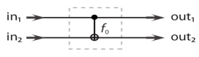
Figure 1: The above figure depicts a simple CNOT transformation conditional on the bit $f_{0}$. The circuit does not apply the gate if $f_{0}=0$ and applies it if $f_{0}=1$.

Figure 1 depicts the “quantum shift register circuit” that implements this transformation (this device is not really a quantum shift register circuit because it does not exploit a set of memory qubits).

Let us incorporate one frame of memory qubits so that the circuit really now becomes a quantum shift register circuit. Consider the circuit in Figure 2. The first two qubits are fed into the device and the second one is the target of a CNOT gate from a future frame of qubits (conditional on the bit $f_{1}$). The two qubits are then stored as two memory qubits (swapped out with what was previously there). On the next cycle, the two qubits are fed out and the first qubit that was previously in memory acts on the second qubit in a frame that is in the past with respect to itself. We would expect the $X$ variable of the first outgoing qubit to propagate one frame into the past with respect to itself and the $Z$ variable of the second incoming qubit to propagate one frame into the future with respect to itself. We make this idea more clear in the below analysis.

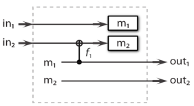
Figure 2: A quantum shift register device that incorporates one frame of memory qubits.

We can analyze this situation with a set of recursive equations. Let $x_{1}\left[n\right]$ denote the bit representation of the $X$ Pauli operator for the first incoming qubit at time $n$ and let $z_{1}\left[n\right]$ denote the bit representation of the $Z$ Pauli operator for the first incoming qubit at time $n$. Let $x_{2}\left[n\right]$ and $z_{2}\left[n\right]$ denote similar quantities for the second incoming qubit at time $n$. Let $m_{1}^{x}\left[n\right]$ denote the bit representation of the $X$ Pauli operator acting on the first memory qubit at time $n$ and let $m_{1}^{z}\left[n\right]$ denote the bit representation of the $Z$ Pauli operator acting on the first memory qubit at time $n$. Let $m_{2}^{x}\left[n\right]$ and $m_{2}^{z}\left[n\right]$ denote similar quantities for the second memory qubit. In the symplectic bit vector notation, we denote the “Z” part of the Pauli operators acting on these four qubits at time $n$ as

$$\mathbf{z}\left[n\right]\equiv\left[\begin{array}[c]{cccc}z_{1}\left[n\right]&z_{2}\left[n\right]&m_{1}^{z}\left[n-1\right]&m_{2}^{z}\left[n-1\right]\end{array}\right],$$

and the “X” part by

$$\mathbf{x}\left[n\right]\equiv\left[\begin{array}[c]{cccc}x_{1}\left[n\right]&x_{2}\left[n\right]&m_{1}^{x}\left[n-1\right]&m_{2}^{x}\left[n-1\right]\end{array}\right].$$

The symplectic vector for the inputs is then

$$\left[\left.\begin{array}[c]{c}\mathbf{z}\left[n\right]\end{array}\right|\begin{array}[c]{c}\mathbf{x}\left[n\right]\end{array}\right].$$ (1)

I prefer this bit notation of Poulin et al. arx2007poulin because it is more flexible for quantum shift register circuits. It allows us to capture the evolution of an arbitrary tensor product of Pauli operators acting on these four qubits at time $n$.

At time $n$, the two incoming qubits and the previous memory qubits from time $n-1$ are fed into the quantum shift register device and the CNOT gate acts on them. The notation in Figure 2 indicates that there is an implicit swap at the end of the operation. The incoming qubits get fed into the memory, and the previous memory qubits get fed out as output. Let $x_{1}^{\prime}\left[n\right]$, $z_{1}^{\prime}\left[n\right]$, $x_{2}^{\prime}\left[n\right]$, and $z_{2}^{\prime}\left[n\right]$ denote the respective output variables. The symplectic transformation for the CNOT gate is

$$\left[\left.\begin{array}[c]{cccc}1&0&0&0\\ 0&1&f_{1}&0\\ 0&0&1&0\\ 0&0&0&1\\ 0&0&0&0\\ 0&0&0&0\\ 0&0&0&0\\ 0&0&0&0\end{array}\right|\begin{array}[c]{cccc}0&0&0&0\\ 0&0&0&0\\ 0&0&0&0\\ 0&0&0&0\\ 1&0&0&0\\ 0&1&0&0\\ 0&f_{1}&1&0\\ 0&0&0&1\end{array}\right].$$

The above matrix postmultiplies the vector in (1) to give the following output vector. We denote the “Z” part of the output Pauli operators acting on these four qubits at time $n$ as

$$\mathbf{z}^{\prime}\left[n\right]\equiv\left[\begin{array}[c]{cccc}m_{1}^{z}\left[n\right]&m_{2}^{z}\left[n\right]&z_{1}^{\prime}\left[n\right]&z_{2}^{\prime}\left[n\right]\end{array}\right],$$

and the “X” part by

$$\mathbf{x}^{\prime}\left[n\right]\equiv\left[\begin{array}[c]{cccc}m_{1}^{x}\left[n\right]&m_{2}^{x}\left[n\right]&x_{1}^{\prime}\left[n\right]&x_{2}^{\prime}\left[n\right]\end{array}\right],$$

with the change of locations corresponding to the implicit swap. The symplectic vector for the outputs is then

$$\left[\left.\begin{array}[c]{c}\mathbf{z}^{\prime}\left[n\right]\end{array}\right|\begin{array}[c]{c}\mathbf{x}^{\prime}\left[n\right]\end{array}\right].$$ (2)

It is simpler to describe the above transformation as a set of recursive “update” equations:

$$x_{1}^{\prime}\left[n\right] =m_{1}^{x}\left[n-1\right],$$

$$z_{1}^{\prime}\left[n\right] =m_{1}^{z}\left[n-1\right]+f_{1}z_{2}\left[n\right],$$

$$x_{2}^{\prime}\left[n\right] =m_{2}^{x}\left[n-1\right],$$

$$z_{2}^{\prime}\left[n\right] =m_{2}^{z}\left[n-1\right],$$

$$m_{1}^{x}\left[n\right] =x_{1}\left[n\right],$$

$$m_{1}^{z}\left[n\right] =z_{1}\left[n\right],$$

$$m_{2}^{x}\left[n\right] =x_{2}\left[n\right]+f_{1}m_{1}^{x}\left[n-1\right],$$

$$m_{2}^{z}\left[n\right] =z_{2}\left[n\right].$$

Some substitutions simplify this set of recursive equations so that it becomes the following set:

$$x_{1}^{\prime}\left[n\right] =x_{1}\left[n-1\right],$$

$$z_{1}^{\prime}\left[n\right] =z_{1}\left[n-1\right]+f_{1}z_{2}\left[n\right],$$

$$x_{2}^{\prime}\left[n\right] =x_{2}\left[n-1\right]+f_{1}x_{1}\left[n-2\right],$$

$$z_{2}^{\prime}\left[n\right] =z_{2}\left[n-1\right].$$

We can transform this set of equations into the “$D$-domain” with the $D$-transform book1999conv . The set transforms as follows:

$$x_{1}^{\prime}\left(D\right) =Dx_{1}\left(D\right),$$

$$z_{1}^{\prime}\left(D\right) =D\left(z_{1}\left(D\right)+f_{1}D^{-1}z_{2}\left(D\right)\right),$$

$$x_{2}^{\prime}\left(D\right) =D\left(x_{2}\left(D\right)+f_{1}Dx_{1}\left(D\right)\right),$$

$$z_{2}^{\prime}\left(D\right) =Dz_{2}\left(D\right).$$

This set of transformations is linear, and we can write them as the following matrix equation:

$$D\left[\left.\begin{array}[c]{cc}1&0\\ f_{1}D^{-1}&1\\ 0&0\\ 0&0\end{array}\right|\begin{array}[c]{cc}0&0\\ 0&0\\ 1&f_{1}D\\ 0&1\end{array}\right].$$

The factor of $D$ accounts for the unit delay necessary to implement this device, but it is not particularly relevant for the purposes of the transformation (we might as well say that this quantum shift register device implements the transformation without the factor of $D$). Postmultiplying the vector

$$\left[\left.\begin{array}[c]{cc}z_{1}\left(D\right)&z_{2}\left(D\right)\end{array}\right|\begin{array}[c]{cc}x_{1}\left(D\right)&x_{2}\left(D\right)\end{array}\right]$$

by the above matrix gives the output vector

$$\left[\left.\begin{array}[c]{cc}z_{1}^{\prime}\left(D\right)&z_{2}^{\prime}\left(D\right)\end{array}\right|\begin{array}[c]{cc}x_{1}^{\prime}\left(D\right)&x_{2}^{\prime}\left(D\right)\end{array}\right].$$

The above transformation confirms our intuition concerning the propagation of $X$ and $Z$ variables. The $D$ term on the right side of the transformation matrix indicates that the $X$ variable of the first qubit propagates one frame into the past with respect to itself, and the $D^{-1}$ term on the left side of the matrix indicates that the $Z$ variable of the second qubit propagates one frame into the future with respect to itself.

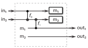
Figure 3: The circuit in the above figure combines the circuits in Figures 1 and 2.

We now consider combining the different quantum shift register circuits together. Suppose that we connect the outputs of the device in Figure 1 to the inputs of the device in Figure 2. Figure 3 depicts the resulting quantum shift register circuit, and it follows that the resulting transformation in the $D$-domain is

$$D\left[\left.\begin{array}[c]{cc}1&0\\ f_{0}+f_{1}D^{-1}&1\\ 0&0\\ 0&0\end{array}\right|\begin{array}[c]{cc}0&0\\ 0&0\\ 1&f_{0}+f_{1}D\\ 0&1\end{array}\right].$$ (3)

Now consider the “two-delay transformation” in Figure 4. The circuit is similar to the one in Figure 2, with the exception that the first outgoing qubit acts on the second incoming qubit and the second incoming qubit is delayed two frames with respect to the first outgoing qubit. We now expect that the $X$ variable propagates two frames into the past, while the $Z$ variable propagates two frames into the future. The transformation should be as follows:

$$D^{2}\left[\left.\begin{array}[c]{cc}1&0\\ f_{2}D^{-1}&1\\ 0&0\\ 0&0\end{array}\right|\begin{array}[c]{cc}0&0\\ 0&0\\ 1&f_{2}D\\ 0&1\end{array}\right].$$ (4)

An analysis similar to the one for the “one-delay” CNOT transformation shows that the circuit indeed implements the above transformation.

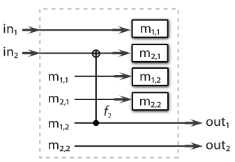
Figure 4: The circuit in the above figure implements a two-delay CNOT transformation.

Let us connect the outputs of the device in Figure 3 to the inputs of the device in Figure 4. The resulting $D$-domain transformation should be the multiplication of the transformation in (3) with that in (4), and an analysis with recursive equations confirms that the transformation is the following one:

$$D^{3}\left[\left.\begin{array}[c]{cc}1&0\\ f_{0}+f_{1}D^{-1}+f_{2}D^{-2}&1\\ 0&0\\ 0&0\end{array}\right|\begin{array}[c]{cc}0&0\\ 0&0\\ 1&f_{0}+f_{1}D+f_{2}D^{2}\\ 0&1\end{array}\right].$$ (5)

The resulting device uses three frames of memory qubits to implement the transformation. This amount of memory seems like it may be too much, considering that the output data only depends on the input from two frames into the past. Is there any way to save on memory consumption?

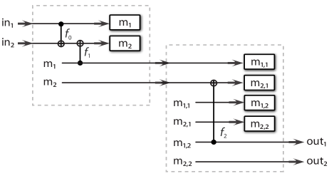
Figure 5: The above circuit connects the outputs of the circuit in Figure 3 to the inputs of the circuit in Figure 4.

First, let us connect the outputs of the circuit in Figure 3 to the inputs of the circuit in Figure 4. Figure 5 depicts the resulting device. In this “combo” device, the target of the CNOT gate conditional on $f_{2}$ does not act on the source of the CNOT gate conditional on $f_{1}$. Therefore, we can commute the “$f_{2}$-gate” with the “$f_{1}$-gate.” Now, we can actually then “commute this gate through the memory” because it does not matter whether this CNOT gate acts on the qubits before they pass through the memory or after they come out. It then follows that the last frame of memory qubits are not necessary because there is no gate that acts on these last qubits. Figure 6 depicts the simplified transformation. It is also straightforward to check that the resulting transformation is as follows:

$$D^{2}\left[\left.\begin{array}[c]{cc}1&0\\ f_{0}+f_{1}D^{-1}+f_{2}D^{-2}&1\\ 0&0\\ 0&0\end{array}\right|\begin{array}[c]{cc}0&0\\ 0&0\\ 1&f_{0}+f_{1}D+f_{2}D^{2}\\ 0&1\end{array}\right],$$ (6)

where the premultiplying delay factor in (6) is now $D^{2}$ instead of $D^{3}$ as in (5).

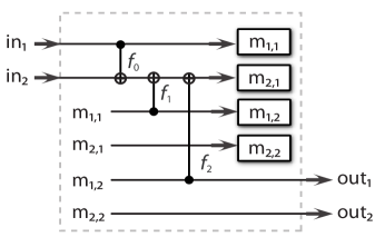
Figure 6: The above circuit reduces the amount of memory required to implement the transformation in (5).

III General Encoding Algorithm

The procedure in the previous section allows us to simplify the circuit by eliminating the last frame of memory qubits. This procedure of determining whether we can “commute gates through the memory” is a general one that we can employ for reducing memory in quantum shift register circuits. In the above example, we can determine the number of frames of memory that are necessary by considering the absolute degree of the polynomial transformation in (5) (without including the $D^{3}$ prefactor). The absolute degree $\left|\deg\right|\left(B\left(D\right)\right)$ of a polynomial matrix $B\left(D\right)$ is

$$\left|\deg\right|\left(B\left(D\right)\right)\equiv\max\left\{d_{1},d_{2}\right\},$$

where

$$d_{1} \equiv\max_{i,j}\left\{\deg\left(\left[B\left(D\right)\right]_{ij}\right)\right\},$$

$$d_{2} \equiv\max_{i,j}\left\{\left|\text{del}\left(\left[B\left(D\right)\right]_{ij}\right)\right|\right\},$$

del$\left(b\left(D\right)\right)$ is the lowest power in the polynomial $b\left(D\right)$, and the absolute degree is modulo any prefactor terms such as the $D^{3}$ in (5). In the case of the transformation in (5), the absolute degree is equal to two, so we should expect to have two frames of memory qubits. Theorem 3 generalizes this idea by showing that the absolute degree of an encoding matrix corresponds to the amount of memory that a CSS quantum convolutional code requires.

The procedure in the previous section demonstrates a general procedure for constructing quantum shift register circuits for quantum convolutional codes. We can break the encoding operation into elementary operations as the Grassl-Rötteler encoding algorithm does ieee2006grassl ; isit2006grassl ; ieee2007grassl ; arx2007wildeEAQCC . The general procedure implements each elementary operation with a quantum shift register circuit, connects the outputs of one quantum shift register circuit to the inputs of the next, and determines if it is possible to “commute gates through memory” as shown in the above example. This procedure produces a quantum shift register encoding circuit that uses the minimal amount of memory.

IV Example of a Quantum Shift Register Encoding Circuit for a CSS Quantum Convolutional Code

Let us consider a simple example of a CSS quantum convolutional code PhysRevA.54.1098 ; PhysRevLett.77.793 . Its stabilizer matrix arxiv2004olliv ; isit2006grassl is as follows:

$$\left[\left.\begin{array}[c]{ccc}0&0&0\\ D&1&1+D\end{array}\right|\begin{array}[c]{ccc}1&D&1+D\\ 0&0&0\end{array}\right].$$ (7)

I now show how to encode the above quantum convolutional code using a slight modification of the Grassl-Rötteler encoding algorithm for CSS codes ieee2007grassl . One begins with the stabilizer matrix for two ancilla qubits per frame:

$$\left[\left.\begin{array}[c]{ccc}0&0&0\\ 0&1&0\end{array}\right|\begin{array}[c]{ccc}1&0&0\\ 0&0&0\end{array}\right].$$

The first ancilla qubit of every frame is in the state $\left|+\right\rangle$ and the second ancilla qubit of every frame is in the state $\left|0\right\rangle$. First send the three qubits through a quantum shift register device that implements a CNOT$\left(3,2\right)\left(1+D^{-1}\right)$. This notation indicates that there is a CNOT gate from the third qubit to the second in the same frame and to the second in a future frame. The stabilizer becomes

$$\left[\left.\begin{array}[c]{ccc}0&0&0\\ 0&1&1+D\end{array}\right|\begin{array}[c]{ccc}1&0&0\\ 0&0&0\end{array}\right].$$ (8)

Then send the three qubits through a quantum shift register device that performs a CNOT$\left(1,2\right)\left(D\right)$ (indicating a CNOT from the first qubit in one frame to the second in a delayed frame) and another quantum shift register device that performs a CNOT$\left(1,3\right)\left(1+D\right)$. The stabilizer becomes

$$\left[\left.\begin{array}[c]{ccc}0&0&0\\ D&1&1+D\end{array}\right|\begin{array}[c]{ccc}1&D&1+D\\ 0&0&0\end{array}\right],$$ (9)

and is now encoded. Note that the above circuit is a “classical” circuit in the sense that it uses only CNOT gates in its implementation. Figure 7 depicts the quantum shift register circuit corresponding to the above operations.

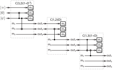
Figure 7: The above circuit implements the set of transformations outlined in (8-9).

It again seems that the circuit in Figure 7 is wasteful in memory consumption. Is there anything we can do to simplify this circuit? First notice that the target qubit of the CNOT gate in the second quantum shift register is the same as the target qubit of the second CNOT gate in the first quantum shift register. It follows that these two gates commute so that we can act with the CNOT gate in the second quantum shift register before acting with the second CNOT gate of the first quantum shift register. But we can do even better. Acting first with the CNOT gate in the second quantum shift register is equivalent to having it act before the first frame of memory qubits gets delayed. Figure 8 depicts this simplification.

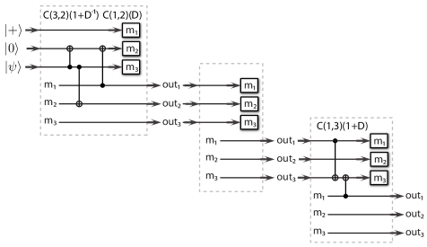
Figure 8: The above figure depicts a simplification of the circuit in Figure 7.

But glancing at Figure 8, it is now clear that the second quantum shift register circuit no longer serves any purpose. We may remove it from the circuit. Figure 9 displays the resulting simplified circuit.

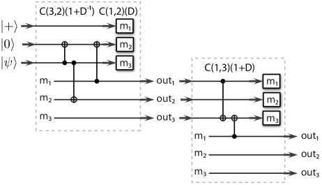
Figure 9: The above figure depicts a simplified version of the circuit in Figure 8 where we have removed the second unnecessary quantum shift register circuit. The above circuit uses less memory than the one in Figure 8, while still effecting the same transformation.

We can apply a similar logic to the two gates in the second quantum shift register of Figure 9 because the two gates there commute with the preceding gates. Performing a similar simplification and elimination of the last frame of memory qubits leads to the final circuit. Figure 10 depicts the quantum shift register circuit that encodes this quantum convolutional code with one frame of memory qubits.

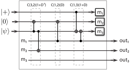
Figure 10: The circuit in the above figure is a quantum shift register encoding circuit for the CSS quantum convolutional code in (7).

The overall encoding matrix for this code is

$$\text{CNOT}\left(3,2\right)\left(1+D^{-1}\right)\text{CNOT}\left(1,2\right)\left(D\right)\text{CNOT}\left(1,3\right)\left(1+D\right)$$

$$=\left[\left.\begin{array}[c]{ccc}1&0&0\\ D&1&D+1\\ D^{-1}+1&0&1\\ 0&0&0\\ 0&0&0\\ 0&0&0\end{array}\right|\begin{array}[c]{ccc}0&0&0\\ 0&0&0\\ 0&0&0\\ 1&D&D+1\\ 0&1&0\\ 0&D^{-1}+1&1\end{array}\right].$$

The absolute degree of the encoding matrix is one, and thus, this CSS code requires one frame of memory qubits. Theorem 3 generalizes this result to show that the memory of the encoding circuit for any CSS quantum convolutional code is given by the absolute degree of the encoding matrix for the circuit.

V Primitive Quantum Shift Register Circuits for CSS Quantum Convolutional Codes

In this section, I outline some basic primitive operations that are useful building blocks for the quantum shift register circuits of CSS (and non-CSS) quantum convolutional codes. I illustrate delay elements and finite-depth CNOT operations.

V.1 Delay Operations

The simplest operation that we can perform with a quantum shift register circuit is to delay one qubit with respect to the others in a given frame. The way to implement this operation is simply to insert a memory element on the qubit that we wish to delay. Figure 11 depicts this delay operation. Suppose that the Pauli operators for the two qubits in the example are as follows (with the convention that the “Z” operators are on the left and the “X” operators are on the right):

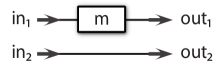
Figure 11: A circuit that implements a simple delay operation on the first qubit in each frame.

$$\left[\left.\begin{array}[c]{cc}1&0\\ 0&1\\ 0&0\\ 0&0\end{array}\right|\begin{array}[c]{cc}0&0\\ 0&0\\ 1&0\\ 0&1\end{array}\right].$$

The circuit in Figure 11 transforms the operators as follows:

$$\left[\left.\begin{array}[c]{cc}D&0\\ 0&1\\ 0&0\\ 0&0\end{array}\right|\begin{array}[c]{cc}0&0\\ 0&0\\ D&0\\ 0&1\end{array}\right].$$

V.2 Building Finite-Depth CNOT Operations

I now show how to generalize the above examples to implement a general CNOT finite-depth operation. Suppose that we have two qubits on which we would like to perform a finite-depth operation . The Pauli operators for these qubits are as follows:

$$\left[\left.\begin{array}[c]{cc}1&0\\ 0&1\\ 0&0\\ 0&0\end{array}\right|\begin{array}[c]{cc}0&0\\ 0&0\\ 1&0\\ 0&1\end{array}\right].$$

A general shift-invariant finite-depth CNOT operation translates the above set of operators to the following set:

$$\left[\left.\begin{array}[c]{cc}1&0\\ f\left(D^{-1}\right)&1\\ 0&0\\ 0&0\end{array}\right|\begin{array}[c]{cc}0&0\\ 0&0\\ 1&f\left(D\right)\\ 0&1\end{array}\right],$$ (10)

where $f\left(D\right)$ is some arbitrary binary polynomial:

$$f\left(D\right)=\sum_{i=0}^{M}f_{i}D^{i}.$$

Theorem 1

The circuit in Figure 12 implements the transformation in (10) and it requires $M$ frames of memory qubits.

Proof. The proof of this theorem uses linear system theoretic techniques by considering symplectic binary vectors that correspond to the Pauli operators for the incoming qubits, the outgoing ones, and the memory qubits. We can formulate a system of recursive equations involving these binary variables similar to how we did for the previous examples. Let us label the bit representations of the $X$ Pauli operators for all the qubits as follows:

$$x_{1}^{\prime},x_{2}^{\prime},m_{1,1}^{x},m_{2,1}^{x},m_{1,2}^{x},m_{2,2}^{x},\ldots,m_{1,M}^{x},m_{2,M}^{x},x_{1},x_{2},$$

where the primed variables are the outputs and the unprimed are the inputs. Let us label the bit representations of the $Z$ Pauli operators similarly:

$$z_{1}^{\prime},z_{2}^{\prime},m_{1,1}^{z},m_{2,1}^{z},m_{1,2}^{z},m_{2,2}^{z},\ldots,m_{1,M}^{z},m_{2,M}^{z},z_{1},z_{2}.$$

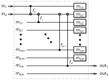
Figure 12: The circuit in the above figure implements the transformation in (10).

The circuit in Figure 12 implements the following set of recursive “X” equations:

$$x_{1}^{\prime}\left[n\right] =m_{1,M}^{x}\left[n-1\right],$$

$$x_{2}^{\prime}\left[n\right] =m_{2,M}^{x}\left[n-1\right],$$

$$m_{1,1}^{x}\left[n\right] =x_{1}\left[n\right],$$

$$m_{2,1}^{x}\left[n\right] =x_{2}\left[n\right]+f_{0}x_{1}\left[n\right]+\sum_{i=1}^{M}f_{i}m_{1,i}^{x}\left[n-1\right],$$

and $\forall i=2\ldots M$,

$$m_{1,i}^{x}\left[n\right] =m_{1,i-1}^{x}\left[n-1\right],$$

$$m_{2,i}^{x}\left[n\right] =m_{2,i-1}^{x}\left[n-1\right].$$

The set of “Z” recursive equations is as follows:

$$z_{1}^{\prime}\left[n\right] =m_{1,M}^{z}\left[n-1\right]+f_{M}\ z_{2}\left[n\right],$$

$$z_{2}^{\prime}\left[n\right] =m_{2,M}^{z}\left[n-1\right],$$

$$m_{1,1}^{z}\left[n\right] =z_{1}\left[n\right]+f_{0}\ z_{2}\left[n\right],$$

$$m_{2,1}^{z}\left[n\right] =z_{2}\left[n\right],$$

and $\forall i=2,\ldots,M$,

$$m_{1,i}^{z}\left[n\right] =m_{1,i-1}^{z}\left[n-1\right]+f_{i-1}\ z_{2}\left[n\right],$$

$$m_{2,i}^{z}\left[n\right] =m_{2,i-1}^{z}\left[n-1\right].$$

Simplifying the “X” equations gives the following two equations:

$$x_{1}^{\prime}\left[n\right] =x_{1}\left[n-M\right],$$

$$x_{2}^{\prime}\left[n\right] =x_{2}\left[n-M\right]+\sum_{i=0}^{M}f_{i}x_{1}\left[n-M-i\right].$$

Simplifying the “Z” equations gives the following two equations:

$$z_{1}^{\prime}\left[n\right] =z_{1}\left[n-M\right]+\sum_{i=0}^{M}f_{i}z_{2}\left[n-M+i\right],$$

$$z_{2}^{\prime}\left[n\right] =z_{2}\left[n-M\right].$$

Applying the $D$-transform to the above gives the following set of equations:

$$x_{1}^{\prime}\left(D\right) =D^{M}x_{1}\left(D\right),$$

$$x_{2}^{\prime}\left(D\right) =D^{M}\left(x_{2}\left(D\right)+\sum_{i=0}^{M}f_{i}D^{i}x_{1}\left(D\right)\right)$$

$$=D^{M}\left(x_{2}\left(D\right)+f\left(D\right)x_{1}\left(D\right)\right),$$

$$z_{1}^{\prime}\left(D\right) =D^{M}\left(z_{1}\left(D\right)+\sum_{i=0}^{M}f_{i}D^{-i}z_{2}\left(D\right)\right)$$

$$=D^{M}\left(z_{1}\left(D\right)+f\left(D^{-1}\right)z_{2}\left(D\right)\right),$$

$$z_{2}^{\prime}\left(D\right) =D^{M}z_{2}\left(D\right).$$

Rewriting the above set of equations as a matrix transformation reveals that it is equivalent to the transformation in (10) (modulo the factor $D^{M}$):

$$\left[\left.\begin{array}[c]{cc}1&0\\ f\left(D^{-1}\right)&1\\ 0&0\\ 0&0\end{array}\right|\begin{array}[c]{cc}0&0\\ 0&0\\ 1&f\left(D\right)\\ 0&1\end{array}\right]D^{M}.$$

Postmultiplying the following vector by the above transformation

$$\left[\left.\begin{array}[c]{cc}z_{1}\left(D\right)&z_{2}\left(D\right)\end{array}\right|\begin{array}[c]{cc}x_{1}\left(D\right)&x_{2}\left(D\right)\end{array}\right],$$

gives the following output vector:

$$\left[\left.\begin{array}[c]{cc}z_{1}^{\prime}\left(D\right)&z_{2}^{\prime}\left(D\right)\end{array}\right|\begin{array}[c]{cc}x_{1}^{\prime}\left(D\right)&x_{2}^{\prime}\left(D\right)\end{array}\right].$$

The circuit in Figure 12 uses $M$ frames of memory qubits ($2M$ actual memory qubits).   

Suppose now that we reverse the direction of the CNOT gates in Figure 12. The result is to perform a shift-invariant finite-depth CNOT operation “conjugate” to that in (10):

$$\left[\left.\begin{array}[c]{cc}1&f\left(D\right)\\ 0&1\\ 0&0\\ 0&0\end{array}\right|\begin{array}[c]{cc}0&0\\ 0&0\\ 1&0\\ f\left(D^{-1}\right)&1\end{array}\right].$$ (11)

It merely switches the roles of the $X$ and $Z$ variables.

Figure 13: The circuit in the above figure implements the transformation in (11). Comparing the circuit in the above figure to the one in Figure 12 reveals that it merely flips the direction of the CNOT gates.

Theorem 2

The circuit in Figure 13 implements the transformation in (11) and requires $M$ frames of memory qubits.

Proof. The proof follows analogously to the above proof by noting that the recursive equations for the “X” and “Z” variables interchange after reversing the direction of the CNOT gates.   

VI Memory Requirements for a CSS Quantum Convolutional Code

Is there a general way for determining how much memory a given code requires just by inspecting its stabilizer matrix? This section answers this question with a theorem that determines the amount of memory that a given CSS quantum convolutional code requires.

Ref. ieee2007grassl defines the individual constraint length, the overall constraint length, and the memory of a quantum convolutional code in analogy to the classical definitions book1999conv . These definitions are analogous to the classical definitions, but there does not seem to be an operational interpretation of them in terms of the actual memory that a given quantum convolutional code requires. We recall those definitions. The constraint length $\nu_{i}$ for row $i$ of the stabilizer matrix is as follows:

$$\nu_{i}\equiv\max_{j}\left\{\max\left\{\deg\left(X_{ij}\left(D\right),\deg\left(Z_{ij}\left(D\right)\right)\right)\right\}\right\}$$

The overall constraint length $\nu$ is the sum of the individual constraint lengths:

$$\nu\equiv\sum_{i}\nu_{i}.$$

The memory $m$ is

$$m\equiv\max_{i}\nu_{i}.$$

We now consider a general technique for computing the memory requirements of a CSS quantum convolutional code, and the resulting formula does not correspond to the above definitions. We exploit the Grassl-Rötteler algorithm for encoding CSS codes ieee2007grassl . This algorithm consists of a sequence of Hadamards, a cascade of CNOTs, another sequence of Hadamards, and another cascade of CNOTs. Here, I give a slightly simplfied algorithm that does not require any Hadamard gates. Suppose that a quantum convolutional code has the following stabilizer matrix:

$$\left[\left.\begin{array}[c]{c}H_{1}\left(D\right)\\ 0\end{array}\right|\begin{array}[c]{c}0\\ H_{2}\left(D\right)\end{array}\right].$$ (12)

We can determine an encoding algorithm by looking at a series of steps to decode the above quantum convolutional code. Assume that the matrices $H_{1}\left(D\right)$ and $H_{2}\left(D\right)$ correspond to noncatastrophic, delay-free check matrices so that they each have a Smith normal form book1999conv ; ieee2007grassl :

$$H_{i}\left(D\right)=A_{i}\left(D\right)\left[\begin{array}[c]{cc}I&0\end{array}\right]B_{i}\left(D\right),$$

where $i=1,2$. If the matrices $A_{i}\left(D\right)$ for $i=1,2$ are not equal to the identity matrix, we can premultiply $H_{i}\left(D\right)$ with the inverse matrix $A_{i}^{-1}\left(D\right)$ for $i=1,2$. These row operations do not affect the error-correcting properties of the quantum convolutional code and give an equivalent code. Let us redefine the matrices $H_{i}\left(D\right)$ as follows:

$$H_{i}\left(D\right)\equiv\left[\begin{array}[c]{cc}I&0\end{array}\right]B_{i}\left(D\right),$$

for $i=1,2$. We can then write each matrix $B_{i}\left(D\right)$ as follows:

$$B_{i}\left(D\right)=\left[\begin{array}[c]{c}H_{i}\left(D\right)\\ \tilde{H}_{i}\left(D\right)\end{array}\right].$$

Consider again the stabilizer matrix in (12). Use CNOT gates to perform the elementary column operations in the matrix $B_{2}^{-1}\left(D\right)$. These operations postmultiply entries in the “X” matrix with the matrix $B_{2}^{-1}\left(D\right)$ and postmultiply entries in the “Z” matrix with the matrix $B_{2}^{T}\left(D^{-1}\right)$. The stabilizer matrix in (12) transforms to the following matrix:

$$\left[\left.\begin{array}[c]{cc}H_{1}\left(D\right)H_{2}^{T}\left(D^{-1}\right)&H_{1}\left(D\right)\tilde{H}_{2}^{T}\left(D^{-1}\right)\\ 0&0\end{array}\right|\begin{array}[c]{cc}0&0\\ I&0\end{array}\right].$$

The matrix $H_{1}\left(D\right)H_{2}^{T}\left(D^{-1}\right)$ is null because the code is a CSS code and satisfies the dual-containing constraint. The stabilizer matrix for the code is then as follows:

$$\left[\left.\begin{array}[c]{cc}0&H_{1}\left(D\right)\tilde{H}_{2}^{T}\left(D^{-1}\right)\\ 0&0\end{array}\right|\begin{array}[c]{cc}0&0\\ I&0\end{array}\right].$$

Compute the Smith form of the matrix $H_{1}\left(D\right)\tilde{H}_{2}^{T}\left(D^{-1}\right)$:

$$H_{1}\left(D\right)\tilde{H}_{2}^{T}\left(D^{-1}\right)=A_{3}\left(D\right)\left[\begin{array}[c]{cc}I&0\end{array}\right]B_{3}\left(D\right).$$

Perform the row operations in $A_{3}^{-1}\left(D\right)$ on the first set of rows. Finally, perform the conjugate CNOT gates corresponding to the entries in $I\oplus B_{3}^{-1}\left(D\right)$—implying that we perform them only on the last few qubits. These operations postmultiply the “X” matrix by the matrix $I\oplus B_{3}^{T}\left(D^{-1}\right)$ and postmultiply the “Z” matrix by the matrix $I\oplus B_{3}^{-1}\left(D\right)$. These operations then produce the following stabilizer matrix:

$$\left[\left.\begin{array}[c]{ccc}0&I&0\\ 0&0&0\end{array}\right|\begin{array}[c]{ccc}0&0&0\\ I&0&0\end{array}\right].$$

We are done at this point. These decoding operations give the following transformations for the “X” matrix:

$$B_{2}^{-1}\left(D\right)\left(I\oplus B_{3}^{T}\left(D^{-1}\right)\right),$$

and the following transformations for the “Z” matrix:

$$B_{2}^{T}\left(D^{-1}\right)\left(I\oplus B_{3}^{-1}\left(D\right)\right).$$

To encode the quantum convolutional code, we perform the above operations in the reverse order. For encoding, the following transformations postmultiply the “X” matrix:

$$E_{X}\left(D\right)\equiv\left(I\oplus\left(B_{3}^{T}\right)^{-1}\left(D^{-1}\right)\right)B_{2}\left(D\right),$$

and the following transformations for the “Z” matrix:

$$E_{Z}\left(D\right)\equiv\left(I\oplus B_{3}\left(D\right)\right)\left(B_{2}^{T}\right)^{-1}\left(D^{-1}\right).$$

The overall encoding matrix is

$$B\left(D\right)\equiv\left[\left.\begin{array}[c]{c}E_{Z}\left(D\right)\\ 0\end{array}\right|\begin{array}[c]{c}0\\ E_{X}\left(D\right)\end{array}\right].$$

(See Ref. ieee2007grassl for a more detailed analysis of this algorithm).

I now give a theorem that determines the amount of memory that a CSS quantum convolutional code requires.

Theorem 3

The number $m$ of frames of memory qubits required for a CSS quantum convolutional code encoded with the Grassl-Rötteler encoding algorithm is upper bounded by the absolute degree of $B\left(D\right)$:

$$m\leq\left|\deg\right|\left(B\left(D\right)\right).$$

Proof. I employ an inductive method of proof. The above encoding algorithm for a CSS quantum convolutional code demonstrates that we only have to consider how CNOT gates combine together in a quantum shift register construction. We can map each elementary CNOT operation to a quantum shift register circuit and connect its outputs to the inputs of the quantum shift register circuit for the next elementary CNOT operation. This technique is wasteful with respect to memory, but the proof of this theorem shows all the ways that we can reduce the amount of memory when combining quantum shift register circuits corresponding to CNOT operations. The result of the theorem then gives a simple formula for determining the amount of memory that a CSS quantum convolutional code requires.

For the base step of the proof, consider that a CNOT gate from qubit $i$ to qubit $j$ in a frame delayed by $l$ requires at most $l$ frames of memory qubits. This result follows by extending the circuit of Figure 4. The polynomial matrix for this CNOT gate that acts on the $i^{\text{th}}$ and $j^{\text{th}}$ qubits is as follows:

$$\left[\left.\begin{array}[c]{cc}1&0\\ D^{-l}&1\\ 0&0\\ 0&0\end{array}\right|\begin{array}[c]{cc}0&0\\ 0&0\\ 1&D^{l}\\ 0&1\end{array}\right],$$

and has an absolute degree of $\left|l\right|$. We abbreviate the above transformation as CNOT$\left(i,j\right)\left(D^{l}\right)$. So the theorem holds for this base case.

Now consider two CNOT gates that have the same source qubits, but the source of one of them acts on a target qubit in a frame delayed by $l_{0}$ and the source of another acts on a target qubit in a frame delayed by $l_{1}$. Suppose, without loss of generality, that $\left|l_{1}\right|>\left|l_{0}\right|$ (these integers can be negative—we should use the term “advanced by” instead of “delayed by” for this case). This combination is a special case of Theorems 1 and 2 and, therefore, we can implement this gate with $\left|l_{1}\right|$ frames of memory qubits. The polynomial matrix for the first CNOT is CNOT$\left(i,j\right)\left(D^{l_{0}}\right)$ and that for the second is CNOT$\left(i,j\right)\left(D^{l_{1}}\right)$. It is straightforward to check that the polynomial matrix for the combined operation is CNOT$\left(i,j\right)\left(D^{l_{0}}+D^{l_{1}}\right)$. The theorem thus holds for this case because the absolute degree of CNOT$\left(i,j\right)\left(D^{l_{0}}+D^{l_{1}}\right)$ is $\left|l_{1}\right|$.

The theorem similarly holds if two CNOT gates have the same source qubits but have target qubits that do not have the same index within their given frame. It also holds if two CNOT gates have the same target qubits but have source qubits that do not have the same index within their given frame. The polynomial matrices for the first case are CNOT$\left(i,j\right)\left(D^{l_{0}}\right)$ and CNOT$\left(i,k\right)\left(D^{l_{1}}\right)$ where WLOG $\left|l_{1}\right|>\left|l_{0}\right|$. These two polynomial matrices commute. One can construct a quantum shift register circuit with the techniques in this paper, and this circuit uses $\left|l_{1}\right|$ frames of memory qubits. It is straightforward to check that the absolute degree of the multiplication of matrices is $\left|l_{1}\right|$. A similar symmetric analysis applies to the other case where the target qubits are the same but the source qubits are different. The main reason the theorem holds in these scenarios is that the polynomial matrix representations of these gates commute with one another. Any time the polynomial representations commute, the corresponding gates in the cascaded quantum shift registers commute through memory so that the maximum amount of frames of memory qubits is equal to the absolute degree of the entries in the multiplication of the polynomial matrices.

Suppose the source qubits and target qubits of the two CNOT gates do not intersect in any way. Then their polynomial matrix representations commute and the amount of memory required is again equal to the absolute degree of the polynomial matrices corresponding to the CNOT gates. An example is CNOT$\left(i,j\right)\left(D^{l_{1}}\right)$ and CNOT $\left(k,l\right)\left(D^{l_{0}}\right)$ where $i\neq j\neq k\neq l$ and WLOG $\left|l_{1}\right|>\left|l_{0}\right|$. One can use the techniques in this paper to construct a combined quantum shift register circuit that requires $\left|l_{1}\right|$ frames of memory qubits.

Suppose the index of source qubit of the first CNOT gate is the same as the index of the target of the second CNOT gate, but the index of the target of the first is different from the index of the source qubit of the second. An example of this scenario is CNOT$\left(i,j\right)\left(D^{l_{0}}\right)$ followed by CNOT$\left(k,i\right)\left(D^{l_{1}}\right)$ where $l_{0}$ and $l_{1}$ are any integers and $\left|l_{1}\right|>\left|l_{0}\right|$ WLOG. The multiplication of the two polynomial matrices gives the following polynomial matrix:

$$\left[\left.\begin{array}[c]{ccc}1&0&D^{-l_{1}}\\ D^{-l_{0}}&1&D^{-\left(l_{1}+l_{0}\right)}\\ 0&0&1\\ 0&0&0\\ 0&0&0\\ 0&0&0\end{array}\right|\begin{array}[c]{ccc}0&0&0\\ 0&0&0\\ 0&0&0\\ 1&D^{l_{0}}&0\\ 0&1&0\\ D^{l_{1}}&0&1\end{array}\right],$$

where the indices $i$, $j$, and $k$ correspond to the first, second, and third columns of the above “Z” and “X” submatrices. It is again straightforward using the technique in this paper to construct a quantum shift register circuit that uses memory equal to the absolute degree of the above polynomial matrix. The circuit uses $\left|l_{1}\right|$ frames of memory qubits in the case that $l_{1}$ is positive and $l_{0}$ is negative and vice versa and uses $\left|l_{1}+l_{0}\right|$ frames of memory qubits in the case that $l_{0}$ and $l_{1}$ are both positive or both negative.

The last scenario to consider is when the index of the source qubit of the first CNOT gate is the same as the index of the target of the second CNOT gate, and the index of the target of the first CNOT gate is the same as the index of the source of the second CNOT gate. An example of this scenario is CNOT$\left(i,j\right)\left(D^{l_{0}}\right)$ followed by CNOT$\left(j,i\right)\left(D^{l_{1}}\right)$, where $l_{0}$ and $l_{1}$ are any integers and $\left|l_{1}\right|>\left|l_{0}\right|$ WLOG. The multiplication of the two polynomial matrices gives the following polynomial matrix:

$$\left[\left.\begin{array}[c]{cc}1&D^{-l_{1}}\\ D^{-l_{0}}&1+D^{-\left(l_{0}+l_{1}\right)}\\ 0&0\\ 0&0\end{array}\right|\begin{array}[c]{cc}0&0\\ 0&0\\ 1+D^{l_{0}+l_{1}}&D^{l_{0}}\\ D^{l_{1}}&1\end{array}\right],$$

where the indices $i$ and $j$ correspond to the first and second columns of the above “Z” and “X” submatrices. It is again straightforward to construct a quantum shift register using the techniques in this paper that uses a number of frames of memory qubits equal to the absolute degree of the polynomial matrix.

The inductive step follows by considering that any arbitrary encoding with CNOTs is a sequence of elementary column operations of the form:

$$B\left(D\right)=B_{\left(1\right)}\left(D\right)B_{\left(2\right)}\left(D\right)\cdots B_{\left(p\right)}\left(D\right),$$

where $p$ is the total number of elementary operations and the above decomposition is a particular decomposition of the matrix $B\left(D\right)$ into elementary operations. Suppose the above encoding matrix requires $m$ frames of memory qubits and $m$ is also the absolute degree of $B\left(D\right)$. Suppose we cascade another elementary encoding operation with matrix representation $B_{\left(p+1\right)}\left(D\right)$. If $B_{\left(p+1\right)}\left(D\right)$ commutes with $B_{\left(p\right)}\left(D\right)$, then it increases the absolute degree of the resulting matrix $B\left(D\right)$ and the memory required for the quantum shift register circuit only if it has a higher absolute degree than $B_{\left(p\right)}\left(D\right)$. The case is thus reducible to the case where it does not commute with $B_{\left(p\right)}\left(D\right)$. So, suppose $B_{\left(p+1\right)}\left(D\right)$ does not commute with $B_{\left(p\right)}\left(D\right)$. There are two ways in which this non-commutativity can happen and I detailed them above. The analysis above for both cases shows that the absolute degree and the number of frames of memory qubits increase by the same amount depending whether $l_{0}$ and $l_{1}$ are positive or negative.   

Corollary 4

A Type I CSS entanglement-assisted quantum convolutional code arx2007wildeEAQCC  encoded with the Grassl-Rötteler encoding algorithm requires $m$ frames of memory qubits, where

$$m\leq\left|\deg\right|\left(B\left(D\right)\right).$$

The matrix $B\left(D\right)$ is the polynomial matrix representation of the encoding operations of the entanglement-assisted code.

Proof. A Type I CSS entanglement-assisted convolutional code is one that has a finite-depth encoding and decoding circuit. It is possible to show that the encoding circuit consists entirely of CNOT gates. The proof proceeds analogously to the proof of the above theorem.   

VII Other Operations in the Finite-Depth Shift-Invariant Clifford Group

CNOT gates are not the only gates that are useful for encoding a quantum convolutional code. The Hadamard gate, the Phase gate, and the controlled-Phase gate are also useful and are in the finite-depth shift-invariant Clifford group isit2006grassl .

There is no need to formulate a primitive quantum shift register circuit for the Hadamard gate or the Phase gate—the implementation is trivial and does not require memory qubits.

The controlled-phase gate is useful for implementation with a quantum shift register circuit because it acts on two qubits. There are two types of a quantum shift register circuit that we can develop with a controlled-Phase gate. The first type is similar to that for the finite-depth CNOT quantum shift register circuit because it involves two qubits per frame. The second type is different because it involves only one qubit per frame.

VII.1 Finite-Depth Controlled-Phase Gate with Two Qubits per Frame

Suppose that we have two qubits on which we would like to perform a finite-depth controlled-Phase gate operation. The Pauli operators for these qubits are as follows:

$$\left[\left.\begin{array}[c]{cc}1&0\\ 0&1\\ 0&0\\ 0&0\end{array}\right|\begin{array}[c]{cc}0&0\\ 0&0\\ 1&0\\ 0&1\end{array}\right].$$

A general shift-invariant finite-depth controlled-Phase gate operation translates the above set of operators to the following set:

$$\left[\left.\begin{array}[c]{cc}1&0\\ 0&1\\ 0&f\left(D\right)\\ f\left(D^{-1}\right)&0\end{array}\right|\begin{array}[c]{cc}0&0\\ 0&0\\ 1&0\\ 0&1\end{array}\right],$$ (13)

where $f\left(D\right)$ is some arbitrary binary polynomial:

$$f\left(D\right)=\sum_{i=0}^{M}f_{i}D^{i}.$$

Theorem 5

The circuit in Figure 14 implements the transformation in (13), and it requires no more than $M$ frames of memory qubits.

Proof. The proof of this theorem is similar to that of the previous theorems. We can formulate a system of recursive equations involving binary variables. Let us label the bit representations of the $X$ Pauli operators for all the qubits as follows:

$$x_{1}^{\prime},x_{2}^{\prime},m_{1,1}^{x},m_{2,1}^{x},m_{1,2}^{x},m_{2,2}^{x},\ldots,m_{1,M}^{x},m_{2,M}^{x},x_{1},x_{2},$$

where the primed variables are the outputs and the unprimed are the inputs. Let us label the bit representations of the $Z$ Pauli operators similarly:

$$z_{1}^{\prime},z_{2}^{\prime},m_{1,1}^{z},m_{2,1}^{z},m_{1,2}^{z},m_{2,2}^{z},\ldots,m_{1,M}^{z},m_{2,M}^{z},z_{1},z_{2}.$$

Figure 14: The circuit in the above figure implements the transformation in (13).

The circuit in Figure 14 implements the following set of recursive “X” equations:

$$x_{1}^{\prime}\left[n\right] =m_{1,M}^{x}\left[n-1\right],$$

$$x_{2}^{\prime}\left[n\right] =m_{2,M}^{x}\left[n-1\right],$$

$$m_{1,1}^{x}\left[n\right] =x_{1}\left[n\right],$$

$$m_{2,1}^{x}\left[n\right] =x_{2}\left[n\right],$$

and $\forall i=2\ldots M$,

$$m_{1,i}^{x}\left[n\right] =m_{1,i-1}^{x}\left[n-1\right],$$

$$m_{2,i}^{x}\left[n\right] =m_{2,i-1}^{x}\left[n-1\right].$$

The set of “Z” recursive equations is as follows:

$$z_{1}^{\prime}\left[n\right] =m_{1,M}^{z}\left[n-1\right]+f_{M}\ x_{2}\left[n\right],$$

$$z_{2}^{\prime}\left[n\right] =m_{2,M}^{z}\left[n-1\right],$$

$$m_{1,1}^{z}\left[n\right] =z_{1}\left[n\right]+f_{0}\ x_{2}\left[n\right],$$

$$m_{2,1}^{z}\left[n\right] =z_{2}\left[n\right]+f_{0}x_{1}\left[n\right]+\sum_{i=1}^{M}f_{i}m_{1,i}^{x}\left[n-1\right],$$

and $\forall i=2,\ldots,M$,

$$m_{1,i}^{z}\left[n\right] =m_{1,i-1}^{z}\left[n-1\right]+f_{i-1}\ x_{2}\left[n\right],$$

$$m_{2,i}^{z}\left[n\right] =m_{2,i-1}^{z}\left[n-1\right].$$

Simplifying the “X” equations gives the following two equations:

$$x_{1}^{\prime}\left[n\right] =x_{1}\left[n-M\right],$$

$$x_{2}^{\prime}\left[n\right] =x_{2}\left[n-M\right].$$

Simplifying the “Z” equations gives the following two equations:

$$z_{1}^{\prime}\left[n\right] =z_{1}\left[n-M\right]+\sum_{i=0}^{M}f_{i}x_{2}\left[n-M+i\right],$$

$$z_{2}^{\prime}\left[n\right] =z_{2}\left[n-M\right]+\sum_{i=0}^{M}f_{i}x_{1}\left[n-M-i\right].$$

Applying the $D$-transform to the above gives the following set of equations:

$$x_{1}^{\prime}\left(D\right) =D^{M}x_{1}\left(D\right),$$

$$x_{2}^{\prime}\left(D\right) =D^{M}x_{2}\left(D\right),$$

$$z_{1}^{\prime}\left(D\right) =D^{M}\left(z_{1}\left(D\right)+\sum_{i=0}^{M}f_{i}D^{-i}x_{2}\left(D\right)\right)$$

$$=D^{M}\left(z_{1}\left(D\right)+f\left(D^{-1}\right)z_{2}\left(D\right)\right),$$

$$z_{2}^{\prime}\left(D\right) =D^{M}z_{2}\left(D\right)+\sum_{i=0}^{M}f_{i}D^{i}x_{1}\left(D\right)$$

$$=D^{M}\left(z_{2}\left(D\right)+f\left(D\right)x_{1}\left(D\right)\right),$$

Rewriting the above set of equations as a matrix transformation reveals that it is equivalent to the transformation in (13):

$$\left[\left.\begin{array}[c]{cc}1&0\\ 0&1\\ 0&f\left(D\right)\\ f\left(D^{-1}\right)&0\end{array}\right|\begin{array}[c]{cc}0&0\\ 0&0\\ 1&0\\ 0&1\end{array}\right]D^{M}.$$

Postmultiplying the following vector by the above transformation

$$\left[\left.\begin{array}[c]{cc}z_{1}\left(D\right)&z_{2}\left(D\right)\end{array}\right|\begin{array}[c]{cc}x_{1}\left(D\right)&x_{2}\left(D\right)\end{array}\right],$$

gives the following output vector:

$$\left[\left.\begin{array}[c]{cc}z_{1}^{\prime}\left(D\right)&z_{2}^{\prime}\left(D\right)\end{array}\right|\begin{array}[c]{cc}x_{1}^{\prime}\left(D\right)&x_{2}^{\prime}\left(D\right)\end{array}\right].$$

 

VII.2 Finite-Depth Controlled-Phase Gate with One Qubit per Frame

Suppose that we have one qubit on which we would like to perform a finite-depth controlled-Phase gate operation. The Pauli operators for this qubit are as follows:

$$\left[\left.\begin{array}[c]{c}1\\ 0\end{array}\right|\begin{array}[c]{c}0\\ 1\end{array}\right].$$

A general shift-invariant finite-depth controlled-Phase gate operation translates the above set of operators to the following set:

$$\left[\left.\begin{array}[c]{c}1\\ f\left(D\right)+f\left(D^{-1}\right)\end{array}\right|\begin{array}[c]{c}0\\ 1\end{array}\right],$$ (14)

where $f\left(D\right)$ is some arbitrary binary polynomial:

$$f\left(D\right)=\sum_{i=1}^{M}f_{i}D^{i}.$$

Theorem 6

The circuit in Figure 15 implements the transformation in (14) and it requires $M$ frames of memory qubits.

Proof. The proof of this theorem is similar to that of the previous theorems. We can formulate a system of recursive equations involving binary variables. Let us label the bit representations of the $X$ Pauli operators for all the qubits as follows:

$$x^{\prime},m_{1}^{x},m_{2}^{x},\ldots,m_{M}^{x},x,$$

where the primed variables are the outputs and the unprimed are the inputs. Let us label the bit representations of the $Z$ Pauli operators similarly:

$$z^{\prime},m_{1}^{z},m_{2}^{z},\ldots,m_{M}^{z},z.$$

Figure 15: The circuit in the above figure implements the transformation in (15).

The circuit in Figure 15 implements the following set of recursive “X” equations:

$$x_{1}^{\prime}\left[n\right] =m_{M}^{x}\left[n-1\right],$$

$$m_{1}^{x}\left[n\right] =x\left[n\right],$$

and $\forall i=2\ldots M$,

$$m_{i}^{x}\left[n\right]=m_{i-1}^{x}\left[n-1\right].$$

The set of “Z” recursive equations is as follows:

$$z^{\prime}\left[n\right] =m_{M}^{z}\left[n-1\right]+f_{M}\ x\left[n\right],$$

$$m_{1}^{z}\left[n\right] =z\left[n\right]+\sum_{i=1}^{M}f_{i}m_{i}^{x}\left[n-1\right],$$

and $\forall i=2,\ldots,M$,

$$m_{i}^{z}\left[n\right]=m_{i-1}^{z}\left[n-1\right]+f_{i-1}\ x\left[n\right].$$

Simplifying the “X” equations gives the following equation:

$$x^{\prime}\left[n\right]=x\left[n-M\right].$$

Simplifying the “Z” equations gives the following equation:

$$z^{\prime}\left[n\right]=z\left[n-M\right]+\sum_{i=1}^{M}f_{i}x\left[n-M+i\right]\\ +\sum_{i=1}^{M}f_{i}x\left[n-M-i\right].$$

Applying the $D$-transform to the above gives the following set of equations:

$$x^{\prime}\left(D\right) =D^{M}x\left(D\right),$$

$$z^{\prime}\left(D\right) =D^{M}\left(z\left(D\right)+\sum_{i=1}^{M}f_{i}D^{-i}x\left(D\right)+\sum_{i=1}^{M}f_{i}D^{i}x\left(D\right)\right)$$

$$=D^{M}\left(z\left(D\right)+\left(f\left(D^{-1}\right)+f\left(D\right)\right)x\left(D\right)\right),$$

Rewriting the above set of equations as a matrix transformation reveals that it is equivalent to the transformation in (13):

$$\left[\left.\begin{array}[c]{c}1\\ f\left(D^{-1}\right)+f\left(D\right)\end{array}\right|\begin{array}[c]{c}0\\ 1\end{array}\right]D^{M}.$$

Postmultiplying the following vector by the above transformation

$$\left[\left.\begin{array}[c]{c}z\left(D\right)\end{array}\right|\begin{array}[c]{c}x\left(D\right)\end{array}\right],$$

gives the following output vector:

$$\left[\left.\begin{array}[c]{c}z^{\prime}\left(D\right)\end{array}\right|\begin{array}[c]{c}x^{\prime}\left(D\right)\end{array}\right].$$

 

VIII Quantum Shift Register Encoding Circuit for the Forney-Grassl-Guha Code

I now present another example of a quantum shift register encoding circuit for a quantum convolutional code. The code that I choose is the Forney-Grassl-Guha code from Section IIIB of Ref. ieee2007forney . The code has three qubits per frame, and its stabilizer matrix is

$$\left[\left.\begin{array}[c]{ccc}1+D&1&1+D\\ 0&D&D\end{array}\right|\begin{array}[c]{ccc}0&D&D\\ 1+D&1+D&1\end{array}\right].$$

We can again employ the Grassl-Rötteler encoding algorithm ieee2006grassl  to determine a sequence of encoding operations for this code. This sequence of encoding operations is

$$H\left(1\right)H\left(2\right)P\left(1\right)\text{C-PHASE}\left(1,3\right)\left(D^{-1}+1+D\right)$$

$$\text{C-PHASE}\left(1,2\right)\left(D^{-1}\right)\text{C-PHASE}\left(2,3\right)\left(1+D+D^{2}\right)$$

$$\text{CNOT}\left(2,3\right)\left(1\right)\text{CNOT}\left(3,2\right)\left(D\right)\text{CNOT}\left(2,3\right)\left(D\right)$$

$$\text{CNOT}\left(1,2\right)\left(1\right)\text{CNOT}\left(1,3\right)\left(1+D\right)\text{CNOT}\left(2,1\right)\left(D\right),$$

where the order of operations goes from left to right and top to bottom, $H\left(i\right)$ is a Hadamard gate on qubit $i$, and $P\left(i\right)$ is a Phase gate on qubit $i$. I use the technique in this paper to cascade several quantum shift register circuits and commute gates through memory. Figure 16 depicts the quantum shift register circuit that encodes the Forney-Grassl-Guha code.

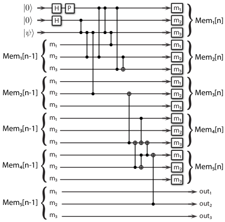
Figure 16: The above circuit encodes the Forney-Grassl-Guha code from Ref. ieee2007forney .

IX General Infinite-Depth Operations

We now turn to infinite-depth operations. Briefly, infinite-depth operations can take a finite-weight Pauli operator to an infinite-weight Pauli operator (similar to the way that an infinite-impulse response filter can have an infinite-duration response to a finite-duration input). Section VI of Ref. arx2007wildeEAQCC  discusses infinite-depth Clifford operations. Here, I give a simplification of that discussion by showing how to implement an arbitrary infinite-depth operation using quantum shift register circuits.

Let $f\left(D\right)$ be some binary polynomial:

$$f\left(D\right)=\sum_{i=0}^{M}f_{i}D^{i}.$$ (15)

Suppose that we have one qubit on which we would like to perform an infinite-depth controlled-NOT operation. The Pauli operators for this qubit are as follows:

$$\left[\left.\begin{array}[c]{c}1\\ 0\end{array}\right|\begin{array}[c]{c}0\\ 1\end{array}\right].$$ (16)

A “Z” infinite-depth operation transforms the logical operators to be as follows:

$$\left[\left.\begin{array}[c]{c}1/f\left(D^{-1}\right)\\ 0\end{array}\right|\begin{array}[c]{c}0\\ f\left(D\right)\end{array}\right],$$ (17)

where $1/f\left(D^{-1}\right)=D^{M}/D^{M}f\left(D^{-1}\right)$.

Theorem 7

The circuit in Figure 17 implements the transformation in (17) and requires $M$ memory qubits.

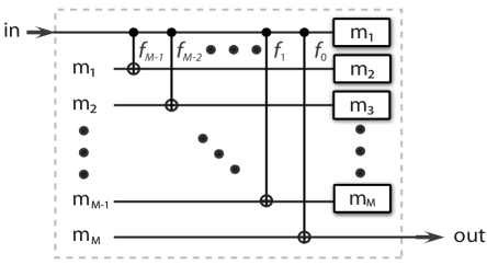
Figure 17: The quantum shift register circuit in the above figure implements the transformation in (17).

Proof. I use a similar linear system theoretic technique that exploits recursive equations and the $D$-transform and assume without loss of generality that the coefficient $f_{M}=1$. We use similar notation as before for the “X” and “Z” variables. We get the following set of “X” recursive equations:

$$x^{\prime}\left[n\right] =m_{M}^{x}\left[n-1\right]+f_{0}x\left[n\right],$$

$$m_{1}^{x}\left[n\right] =x\left[n\right],$$

and $\forall i=2,\ldots,M$,

$$m_{i}^{x}\left[n\right]=m_{i-1}^{x}\left[n-1\right]+f_{M-i+1}x\left[n\right].$$

The “Z” recursive equations are as follows:

$$z^{\prime}\left[n\right] =m_{M}^{z}\left[n-1\right],$$

$$m_{1}^{z}\left[n\right] =z\left[n\right]+\sum_{i=0}^{M-1}f_{i}m_{M-i}^{z}\left[n-1\right],$$

and $\forall i=2\ldots M$,

$$m_{i}^{z}\left[n\right]=m_{i-1}^{z}\left[n-1\right].$$

The first set of “X” recursive equations reduces to the following equation by substitution:

$$x^{\prime}\left[n\right]=\sum_{i=0}^{M}f_{i}x\left[n-i\right].$$ (18)

We can reduce the “Z” equations by first noticing that we can rewrite the equation for $m_{1}^{z}$ as follows:

$$m_{1}^{z}\left[n\right]+f_{M-1}m_{1}^{z}\left[n-1\right]=z\left[n\right]+\sum_{i=0}^{M-2}f_{i}m_{M-i}^{z}\left[n-1\right].$$

We can use the other memory equations to iterate this procedure, and we end up with

$$\sum_{i=0}^{M}f_{M-i}m_{1}^{z}\left[n-i\right]=z\left[n\right].$$

Noting that

$$z^{\prime}\left[n\right]=m_{1}\left[n-M\right],$$

and using shift-invariance, the above equation becomes

$$\sum_{i=0}^{M}f_{i}z^{\prime}\left[n+i\right]=z\left[n\right].$$ (19)

Applying the $D$-transform to (18) gives the following equation:

$$x^{\prime}\left(D\right)=\sum_{i=0}^{M}f_{i}D^{i}x\left(D\right)=f\left(D\right)x\left(D\right).$$

Applying the $D$-transform to (19) gives

$$\sum_{i=0}^{M}f_{i}D^{-i}z^{\prime}\left(D\right) =z\left(D\right)$$

$$\Rightarrow f\left(D^{-1}\right)z^{\prime}\left(D\right) =z\left(D\right)$$

$$\Rightarrow z^{\prime}\left(D\right) =\frac{1}{f\left(D^{-1}\right)}z\left(D\right).$$

Rewriting the above set of transformations as a matrix shows that it is equivalent to the desired transformation in (17):

$$\left[\begin{array}[c]{cc}z\left(D\right)&x\left(D\right)\end{array}\right]\left[\begin{array}[c]{cc}1/f\left(D^{-1}\right)&0\\ 0&f\left(D\right)\end{array}\right]=\left[\begin{array}[c]{cc}z^{\prime}\left(D\right)&x^{\prime}\left(D\right)\end{array}\right].$$

 

Another infinite-depth operation is an “X” infinite-depth operation. It transforms the bit representations in (16) to the following bit representations:

$$\left[\left.\begin{array}[c]{c}0\\ f\left(D\right)\end{array}\right|\begin{array}[c]{c}1/f\left(D^{-1}\right)\\ 0\end{array}\right],$$ (20)

where $f\left(D\right)$ is defined in (15) and $1/f\left(D^{-1}\right)=D^{M}/D^{M}f\left(D^{-1}\right)$.

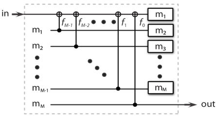
Figure 18: The quantum shift register circuit in the above figure implements the transformation in (20).

Theorem 8

The circuit in Figure 18 implements the transformation in (20) and requires $M$ memory qubits.

Proof. The proof proceeds analogously to the proof of Theorem 7 with the “X” and “Z” variables switching roles because the directionality of the CNOT gates in the circuit in Figure 18 reverses.   

X Memory Requirements for Type II CSS Entanglement-Assisted Quantum Convolutional Codes

Our last contribution is a formula for the amount of memory that a Type II CSS entanglement-assisted quantum convolutional code. A Type II CSS entanglement-assisted quantum convolutional code is one that uses infinite-depth operations, outlined in the previous section, in the encoding circuit arx2007wildeEAQCC .

A particular diagonal matrix $\Gamma_{2}\left(D\right)$ is the essential matrix that determines the infinite-depth operations for a Type II entanglement-assisted code (See Section VII of Ref. arx2007wildeEAQCC ). Each entry on the diagonal corresponds to an infinite-depth operation, similar to the polynomial in (17) and (20). Therefore, the amount of memory that these infinite-depth operations require is

$$m_{1}\equiv\max_{i}\left\{\left|\deg\right|\left(\left[\Gamma_{2}\left(D\right)\right]_{ii}\right)\right\}.$$

Suppose a qubit does not have the maximum absolute degree. Alice should delay this qubit by the difference between that qubit’s absolute degree and the maximum absolute degree so that each qubit lines up properly when output from the infinite-depth encoding operations. Note that it is not possible to commute through memory any gates occurring after an infinite-depth operation.

The structure of the encoding circuit for the Type II entanglement-assisted codes consists of three layers. The first layer is a set of finite-depth CNOT operations characterized by a matrix $L\left(D\right)$ (See Section VII of Ref. arx2007wildeEAQCC ), the second layer consists of the infinite-depth operations, and the third layer is another set of finite-depth CNOT operations that we name $B\left(D\right)$. It is possible to show that we can implement these encoding circuits with CNOT gates only, as we did in Section VI for CSS quantum convolutional codes. Thus, it is straightforward to determine the amount of memory that a Type II CSS entanglement-assisted quantum convolutional code requires, using Theorem 3 and the above upper bound $m_{1}$

Corollary 9

The amount of memory that a Type II CSS entanglement-assisted quantum convolutional code requires is upper bounded by the following quantity:

$$m_{1}+\left|\deg\right|\left(L\left(D\right)\right)+\left|\deg\right|\left(B\left(D\right)\right).$$

XI Conclusion

I have developed the theory for a quantum shift register circuit. These circuits can encode and decode quantum convolutional codes. The two important contributions of this paper are the technique for cascading quantum shift register circuits and the formulas for the memory required by a CSS quantum convolutional code. Quantum shift register circuits should be useful for experimentalists wishing to demonstrate the operation of a quantum convolutional code.

Some interesting open questions remain. I have not yet determined the amount of memory that a general (non-CSS) code requires. The proof technique of Theorem 3 does not extend to combinations of controlled-Phase and controlled-NOT gates because they combine differently from the way that cascades of controlled-NOT gates combine. It might also be interesting to study the entanglement structure of states that are input to a quantum shift register circuit, in a way similar to the observation in Ref. arx2008wildeOEA  concerning the relation of an entanglement measure to an entanglement-assisted code.

- [1] Frank Gaitan. Quantum Error Correction and Fault Tolerant Quantum Computing. CRC Press, Taylor and Francis Group, 2008.
- [2] A. Robert Calderbank and Peter W. Shor. Good quantum error-correcting codes exist. Physical Review A, 54(2):1098–1105, August 1996.
- [3] Andrew M. Steane. Error correcting codes in quantum theory. Physical Review Letters, 77(5):793–797, July 1996.
- [4] Daniel Gottesman. Stabilizer Codes and Quantum Error Correction. PhD thesis, California Institute of Technology, 1997.
- [5] A. Robert Calderbank, Eric M. Rains, Peter W. Shor, and N. J. A. Sloane. Quantum error correction and orthogonal geometry. Physical Review Letters, 78(3):405–408, January 1997.
- [6] A. Robert Calderbank, Eric M. Rains, Peter W. Shor, and N. J. A. Sloane. Quantum error correction via codes over GF(4). IEEE Transactions on Information Theory, 44:1369–1387, 1998.
- [7] Paolo Zanardi and Mario Rasetti. Noiseless quantum codes. Physical Review Letters, 79(17):3306–3309, October 1997.
- [8] Paolo Zanardi and Mario Rasetti. Error avoiding quantum codes. Modern Physics Letters B, 11:1085–1093, 1997.
- [9] Daniel A. Lidar, Isaac L. Chuang, and K. Birgitta Whaley. Decoherence-free subspaces for quantum computation. Physical Review Letters, 81(12):2594–2597, September 1998.
- [10] David Kribs, Raymond Laflamme, and David Poulin. Unified and generalized approach to quantum error correction. Physical Review Letters, 94(18):180501, 2005.
- [11] David W. Kribs, Raymond Laflamme, David Poulin, and Maia Lesosky. Operator quantum error correction. Quantum Information & Computation, 6:383–399, 2006.
- [12] David Poulin. Stabilizer formalism for operator quantum error correction. Physical Review Letters, 95(23):230504, 2005.
- [13] Min-Hsiu Hsieh, Igor Devetak, and Todd A. Brun. General entanglement-assisted quantum error-correcting codes. Physical Review A, 76:062313, 2007.
- [14] Peter W. Shor. Scheme for reducing decoherence in quantum computer memory. Physical Review A, 52(4):R2493–R2496, October 1995.
- [15] Markus Grassl and Martin Rötteler. Noncatastrophic encoders and encoder inverses for quantum convolutional codes. In IEEE International Symposium on Information Theory (quant-ph/0602129), pages 1109–1113, Seattle, Washington, USA, July 2006.
- [16] Mark M. Wilde and Todd A. Brun. Entanglement-assisted quantum convolutional coding. arXiv:0712.2223, 2007.
- [17] Markus Grassl and Martin Rötteler. Quantum convolutional codes: Encoders and structural properties. In Forty-Fourth Annual Allerton Conference, pages 510–519, Allerton House, UIUC, Illinois, USA, September 2006.
- [18] Markus Grassl and Martin Rötteler. Constructions of quantum convolutional codes. In IEEE International Symposium on Information Theory, pages 816–820, Nice, France, June 2007.
- [19] Harold Ollivier and Jean-Pierre Tillich. Quantum convolutional codes: Fundamentals. arXiv:quant-ph/0401134, 2004.
- [20] Mark M. Wilde, Hari Krovi, and Todd A. Brun. Convolutional entanglement distillation. arXiv:0708.3699, 2007.
- [21] Harold Ollivier and Jean-Pierre Tillich. Description of a quantum convolutional code. Physical Review Letters, 91(17):177902, October 2003.
- [22] G. David Forney and Saikat Guha. Simple rate-1/3 convolutional and tail-biting quantum error-correcting codes. In IEEE International Symposium on Information Theory (arXiv:quant-ph/0501099), pages 1028–1032, September 2005.
- [23] G. David Forney, Markus Grassl, and Saikat Guha. Convolutional and tail-biting quantum error-correcting codes. IEEE Transactions on Information Theory, 53:865–880, 2007.
- [24] Salah A. Aly, Markus Grassl, Andreas Klappenecker, Martin Rötteler, and Pradeep Kiran Sarvepalli. Quantum convolutional BCH codes. In 10th Canadian Workshop on Information Theory (arXiv:quant-ph/0703113), pages 180–183, 2007.
- [25] Salah A. Aly, Andreas Klappenecker, and Pradeep Kiran Sarvepalli. Quantum convolutional codes derived from Reed-Solomon and Reed-Muller codes. In International Symposium on Information Theory (arXiv:quant-ph/0701037), pages 821–825, Nice, France, June 2007.
- [26] Mark M. Wilde and Todd A. Brun. Unified quantum convolutional coding. In IEEE International Symposium on Information Theory (arXiv:0801.0821), July 2008.
- [27] Mark M. Wilde and Todd A. Brun. Quantum convolutional coding with shared entanglement: General structure. arXiv:0807.3803, 2008.
- [28] Mark M. Wilde and Todd A. Brun. Extra entanglement reduces memory demand in quantum convolutonal coding. Physical Review A, To appear, 2009.
- [29] Rolf Johannesson and Kamil Sh. Zigangirov. Fundamentals of Convolutional Coding. Wiley-IEEE Press, 1999.
- [30] Tom Richardson and Rüdiger Urbanke. Modern Coding Theory. Cambridge University Press, March 2008.
- [31] Andrew J. Viterbi. Error bounds for convolutional codes and an asymptotically optimum decoding algorithm. IEEE Transactions on Information Theory, 13:260–269, 1967.
- [32] Kenneth S. Andrews, Dariush Divsalar, Sam Dolinar, Jon Hamkins, Christopher R. Jones, and Fabrizio Pollara. The development of turbo and LDPC codes for deep space applications. Proceedings of the IEEE, Special Issue on “Technical Advances in Deep Space Communications and Tracking”, 95(11):2142–2156, November 2007.
- [33] Thomas Kalaith. Linear Systems. Prentice-Hall, Inc., Englewood Cliffs, New Jersey, USA, 1980.
- [34] Markus Grassl and Thomas Beth. Cyclic quantum error-correcting codes and quantum shift registers. Proceedings of the Royal Society A, 456(2003):2689–2706, November 2000.
- [35] Jae-Weon Lee, Eok Kyun Lee, Jaewan Kim, and Soonchil Lee. Quantum shift register. arXiv:quant-ph/0112107, December 2001.
- [36] J. H. Park, J. H. Kang, T. B. Jung, K. R. Jung, C. H. Kim, Y. H. Kim, S. S. Choi, and T. S. Hahn. Low error operation of a 4 stage single flux quantum shift register built with Y-Ba-Cu-0 bicrystal josephson junctions. IEEE Transations on Applied Superconductivity, 11(1):625–628, March 2001.
- [37] David Poulin, Jean-Pierre Tillich, and Harold Ollivier. Quantum serial turbo-codes. arXiv:0712.2888, 2007.
- [38] Sougato Bose. Quantum communication through an unmodulated spin chain. Physical Review Letters, 91(20):207901, November 2003.
- [39] Sougato Bose. Quantum communication through spin chain dynamics: an introductory overview. Contemporary Physics, 48(1):13–30, January 2007.
- [40] Emanuel Knill, Raymond Laflamme, and Gerard J. Milburn. A scheme for efficient quantum computation with linear optics. Nature, 409:46–52, 2001.
- [41] Michael A. Nielsen and Isaac L. Chuang. Quantum Computation and Quantum Information. Cambridge University Press, 2000.
- [42] Mark M. Wilde and Todd A. Brun. Optimal entanglement formulas for entanglement-assisted quantum coding. Physical Review A, 77:064302, 2008.