A unified model for Sierpinski networks with scale-free scaling and small-world effect

Abstract

In this paper, we propose an evolving Sierpinski gasket, based on which we establish a model of evolutionary Sierpinski networks (ESNs) that unifies deterministic Sierpinski network [Eur. Phys. J. B 60, 259 (2007)] and random Sierpinski network [Eur. Phys. J. B 65, 141 (2008)] to the same framework. We suggest an iterative algorithm generating the ESNs. On the basis of the algorithm, some relevant properties of presented networks are calculated or predicted analytically. Analytical solution shows that the networks under consideration follow a power-law degree distribution, with the distribution exponent continuously tuned in a wide range. The obtained accurate expression of clustering coefficient, together with the prediction of average path length reveals that the ESNs possess small-world effect. All our theoretical results are successfully contrasted by numerical simulations. Moreover, the evolutionary prisoner’s dilemma game is also studied on some limitations of the ESNs, i.e., deterministic Sierpinski network and random Sierpinski network.

1 Introduction

In the last few years, complex networks have attracted a growing interest from a wide circle of researchers [1, 2, 3, 4]. The reason for this boom is that complex networks describe various systems in nature and society, such as the World Wide Web (WWW), the Internet, collaboration networks, and sexual network, and so on. Extensive empirical studies have revealed that real-life systems have in common at least two striking statistical properties: power-law degree distribution [5], small-world effect [6] including small average path length (APL) and high clustering coefficient. In order to mimic real-word systems with above mentioned common characteristics, a wide variety of models have been proposed [1, 2, 3, 4]. At present, it is still an active direction to construct models reproducing the structure and statistical characteristics of real systems.

In our previous papers, on the basis of the well-known Sierpinski fractal (or Sierpinski gasket), we have proposed a deterministic network called deterministic Sierpinski network (DSN) [7], and a stochastic network named random Sierpinski network (RSN) [8], respectively. Both the DSN and RSN possess good topological properties observed in some real systems. In this paper, we suggest a general scenario for constructing evolutionary Sierpinski networks (ESNs) controlled by a parameter $q$. The ESNs can also result from Sierpinski gasket and unify the DSN and RSN to the same framework, i.e., the DSN and RSN are special cases of RSNs. The ESNs have a power-law degree distribution, a very large clustering coefficient, and a small intervertex separation. The degree exponent of ESNs is changeable between $2$ and $3$. Moreover, we introduce a generating algorithm for the ESNs which can realize the construction of our networks. In the end, the cooperation behavior of the evolutionary prisoner’s dilemma game on two limiting cases (i.e., DSN and RSN) of the ESNs is discussed.

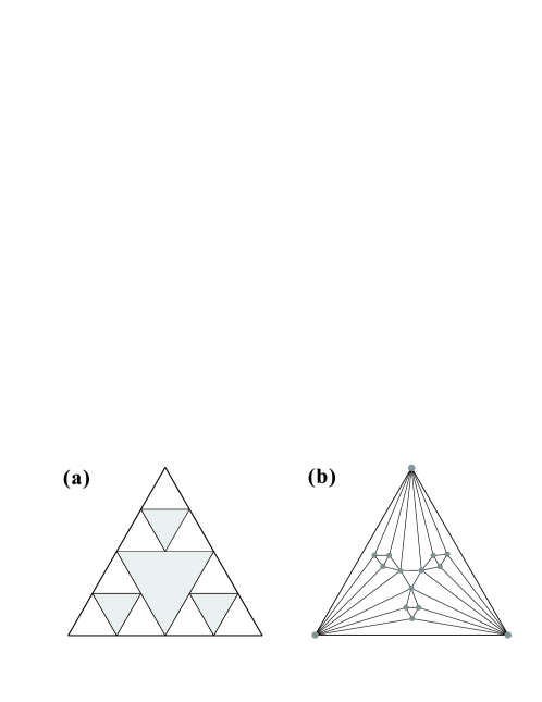
Figure 1: The first two stages of construction of the Sierpinski gasket (a) and its corresponding network (b).

2 Brief introduction to deterministic and random Sierpinski networks

We first introduce Sierpinski gasket, which is also known as Sierpinski triangle. The classical Sierpinski gasket denoted as $S_{t}$ after $t$ generations, is constructed as follows [9, 10]: start with an equilateral triangle, and denote this initial configuration as $S_{0}$. Perform a bisection of the sides forming four small copies of the original triangle, and remove the interior triangles to get $S_{1}$. Repeat this procedure recursively in the three remaining copies to obtain $S_{2}$, see Fig. 1(a). In the infinite $t$ limit, we obtain the famous Sierpinski gasket $S_{t}$. From Sierpinski gasket we can easily construct a network, called deterministic Sierpinski network, with sides of the removed triangles mapped to nodes and contact to edges between nodes [7]. For uniformity, the three sides of the initial equilateral triangle at step 0 also correspond to three different nodes. Figure 1(b) shows a network based on $S_{2}$.

Analogously, one can construct the random Sierpinski network [8] derived from the stochastic Sierpinski gasket, which is a random variant of the deterministic Sierpinski gasket. The initial configuration of the random Sierpinski gasket is the same as the deterministic Sierpinski triangle. Then in each of the subsequent generations, an equilateral triangle is chosen randomly, for which bisection and removal are performed to form three small copies of it. The sketch map for the random fractal is shown in the left panel of Fig. 2. From this fractal we can easily establish the random Sierpinski network with sides of the removed triangles mapped to nodes and contact to links between nodes. The right panel of Fig. 2 gives a network derived from the random Sierpinski gasket.

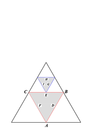
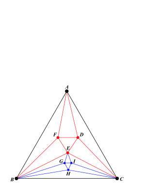
Figure 2: (Color online) The sketch maps for the construction of random Sierpinski gasket (left panel) and its corresponding network (right panel).

3 Unifying model and its iterative algorithm

In this section, we introduce an evolving unified model for the deterministic and random Sierpinski networks. First we give a new variation, called evolving Sierpinski gasket (ESG), for the Sierpinski gasket. The initial configuration of the ESG is the same as the deterministic Sierpinski gasket. Then in each of the subsequent generations, for each equilateral triangle, with probability $q$, bisection and removal are performed to form three small copies of it. In the infinite generation limit, the ESG is obtained. In a special case $q=1$, the ESG is reduced to the classic deterministic Sierpinski gasket. If $q$ approaches but is not equal to $0$, it coincides with the random Sierpinski gasket described in Ref. [8]. The proposed unified model is derived from this ESG: nodes represent the sides of the removed triangles and edges correspond to contact relationship. As in the construction of the deterministic and random Sierpinski networks [7, 8], the three sides of the initial equilateral triangle (at step 0) of the ESG are also mapped to three different nodes.

In the construction process of the ESG, for each equilateral triangle at arbitrary generation, once we perform a bisection of its sides and remove the central down pointing triangle, three copies of it are formed. When building the unifying network model, it is equivalent that for each group of three newly-added nodes, three new triangles are generated, which may create new nodes in the subsequent generations. According to this, we can introduce an iterative algorithm to create the ESNs. Using the proposed algorithm one can write a computer program conveniently to simulate the networks and study their properties.

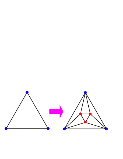
Figure 3: (Color online) Iterative construction method for the network.

We denote the ESNs after $t$ ($t\geq 0$) iterations by $EW(t)$, then the proposed algorithm to create ESNs is as follows. Initially $(t=0)$, $EW(0)$ has three nodes forming a triangle. At step 1, with probability $q$, we add three nodes into the original triangle. These three new nodes are connected to one another shaping a new triangle, and both ends of each edge of the new triangle are linked to a node of the original triangle. Thus we obtain $EW(1)$, see Fig. 3. For $t\geq 1$, $EW(t)$ is obtained from $EW(t-1)$. For the convenience of description, we give the following definition: for each existing triangle in $EW(t-1)$, if there is no node in its interior and among its three nodes there is only one youngest node (i.e., the other two are strictly elder than it), we call it an active triangle (with the initial triangle as an exception). At step $t-1$, for each existing active triangle, with probability $q$ it is replaced by the connected cluster on the right of Fig. 3, then $EW(t)$ is produced. The growing process is repeated until the network reaches a desired order. When $q=1$, the network is exactly the same as the DSN [7]. If $q<1$, the network grows randomly. Especially, as $q$ approaches zero and does not equal zero, the network is reduced to the RSN studied in detail in Ref. [8].

Next we compute the order (number of all nodes) and size (number of all edges) of $EW(t)$. Denote $L_{\Delta}(t)$ as the number of active triangles at step $t$. Then, $L_{\Delta}(0)=1$. By construction, we can easily derive that $L_{\Delta}(t)=(1+2q)^{t}$. Let $L_{v}(t)$ and $L_{e}(t)$ be the number of nodes and edges created at step $t$, respectively. Note that each active triangle in $EW(t-1)$ will (see Fig. 3) lead to three new nodes and nine new edges in $EW(t)$ with probability $q$. Then, at step $1$, we add expected $L_{v}(1)=3q$ new nodes and $L_{e}(1)=9q$ new edges to $EW(0)$. After simple calculations, one can obtain that at step $t_{i}$ $(t_{i}>1)$ the number of newly-born nodes and edges is $L_{v}(t_{i})=3q\,L_{\Delta}(t_{i}-1)=3q(1+2q)^{t_{i}-1}$ and $L_{e}(t_{i})=9q\,L_{\Delta}(t_{i}-1)=9q(1+2q)^{t_{i}-1}$, respectively. Thus the average number of total nodes $N_{t}$ and edges $E_{t}$ present at step $t$ is

$$N_{t}=3+\sum_{t_{i}=1}^{t}L_{v}(t_{i})=\frac{3(1+2q)^{t}+3}{2}$$ (1)

and

$$E_{t}=3+\sum_{t_{i}=1}^{t}L_{e}(t_{i})=\frac{9(1+2q)^{t}-3}{2},$$ (2)

respectively. So for large $t$, the average degree $\overline{k_{t}}=\frac{2E_{t}}{N_{t}}$ is approximately $6$. Obviously, we have $E_{t}=3N_{t}-6$. Moreover, according to the connection rule, arbitrary two edges in the ESNs never cross each other. Thus, the class of networks under consideration are maximal planar networks (or graphs) [11].

4 Relevant characteristics of the Networks

In the following we will study the topology properties of $EW(t)$, in terms of degree distribution, clustering coefficient, and average path length.

4.1 Degree distribution

When a new node $i$ is added to the network at step $t_{i}$ $(t_{i}\geq 1)$, it has a degree of $4$. Let $L_{\vartriangle}(i,t)$ be the expected number of active triangles at step $t$ that will create new nodes connected to the node $i$ at step $t+1$. Then at step $t_{i}$, $L_{\vartriangle}(i,t_{i})=1$. From the iterative generation process of the network, one can see that at any subsequent step each two new neighbors of $i$ generate two new active triangles involving $i$, and one of its existing active triangles is deactivated simultaneously. We define $k_{i}(t)$ as the degree of node $i$ at time $t$, then the relation between $k_{i}(t)$ and $L_{\vartriangle}(i,t)$ satisfies:

$$L_{\vartriangle}(i,t)=\frac{k_{i}(t)-2}{2}.$$ (3)

Now we compute $L_{\vartriangle}(i,t)$. By construction, $L_{\vartriangle}(i,t)=(1+q)L_{\vartriangle}(i,t-1)$. Considering the initial condition $L_{\vartriangle}(i,t_{i})=1$, we can derive $L_{\vartriangle}(i,t)=(1+q)^{t-t_{i}}$. Then at time $t$, the degree of vertex $i$ becomes

$$k_{i}(t)=2(1+q)^{t-t_{i}}+2.$$ (4)

Since the degree of each node has been obtained explicitly as in Eq. (4), we can get the degree distribution via its cumulative distribution [3], i.e., $P_{\rm cum}(k)=\sum_{k^{\prime}\geq k}N(k^{\prime},t)/N_{t}\sim k^{1-\gamma}$, where $N(k^{\prime},t)$ denotes the number of nodes with degree $k^{\prime}$. The detailed analysis is given as follows. For a degree $k=2(1+q)^{t-m}+2$, there are $L_{v}(m)=3q(1+2q)^{m-1}$ nodes with this exact degree, all of which were born at step $m$. All nodes born at time $m$ or earlier have this or a higher degree. So we have

$$\sum_{k^{\prime}\geq k}N(k^{\prime},t)=4+\sum_{s=1}^{m}L_{v}(s)=\frac{3(1+2q)^{m}+3}{2}.$$ (5)

Thus, the cumulative degree distribution is give by

$$P_{\rm cum}(k)=\frac{1}{N_{t}}\sum_{k^{\prime}\geq k}N(k^{\prime},t)=\frac{3(1+2q)^{m}+3}{3(1+2q)^{t}+3}.$$ (6)

Substituting for $m$ in this expression using $m=t-\frac{\ln\frac{k-2}{2}}{\ln(1+q)}$ gives

$$P_{\rm cum}(k)=\frac{3(1+2q)^{t}\cdot 2^{\frac{\ln(1+2q)}{\ln(1+q)}}(k-2)^{-\frac{\ln(1+2q)}{\ln(1+q)}}+3}{3(1+2q)^{t}+3}.$$ (7)

When $t$ is large enough, one can obtain

$$P_{\rm cum}(k)\approx 2^{\frac{\ln(1+2q)}{\ln(1+q)}}(k-2)^{-\frac{\ln(1+2q)}{\ln(1+q)}}.$$ (8)

So the degree distribution follows a power-law form $P(k)\sim k^{-\gamma}$ with the exponent $\gamma=1+\frac{\ln(1+2q)}{\ln(1+q)}$. Note that the degree exponent $\gamma$ is a continuous function of $q$, and belongs to the interval $(1+\frac{\ln 3}{\ln 2},3]$. As $q$ decreases from 1 to 0, $\gamma$ increases from $1+\frac{\ln 3}{\ln 2}$ to $3$. In the two limitations, i.e., $q=1$ and $q\rightarrow 0$ (but $q\neq 0$), the evolutionary Sierpinski networks reduce to the deterministic Sierpinski network [7] and its stochastic variant [8], respectively. Figure 4 shows, on a logarithmic scale, the scaling behavior of the cumulative degree distribution $P_{\rm cum}(k)$ for different values of $q$. Numerical simulation agrees well with the analytical result.

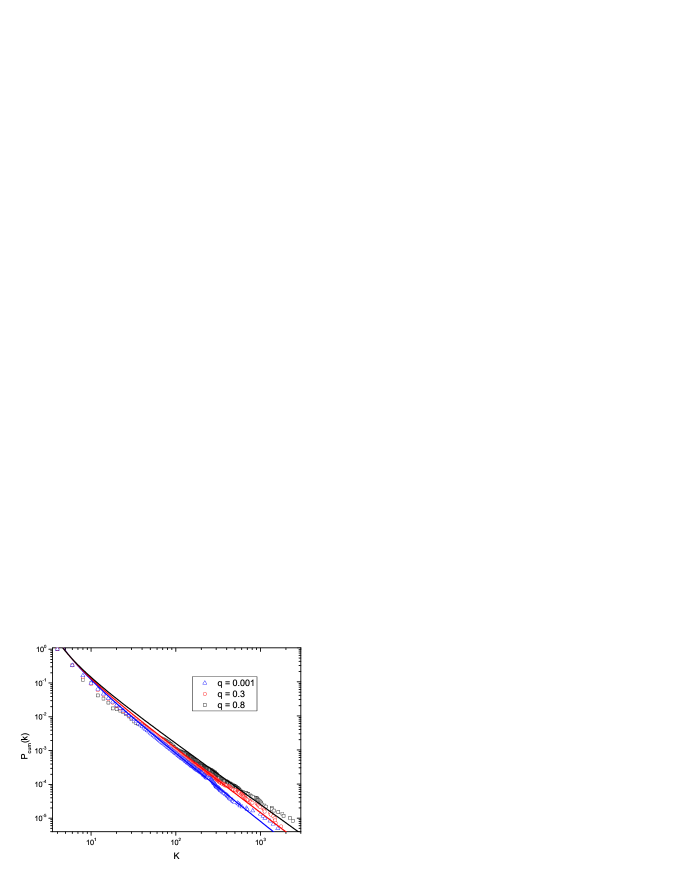
Figure 4: (Color online) The cumulative degree distribution $P_{\rm cum}(k)$ at various $q$ values. The evolutionary steps of simulated network for $q=0.8$, $q=0.3$, and $q=0.001$, are $t=12$, $t=26$, and $t=200000$, respectively. The three lines are the theoretical results as provided by Eq. (8). All data are from the average of ten independent simulations.

4.2 Clustering coefficient

In a network, the clustering coefficient [6] $C_{i}$ of node $i$ is defined as the ratio between the number of edges $e_{i}$ that actually exist among the $k_{i}$ neighbors of node $i$ and its maximum possible value $k_{i}(k_{i}-1)/2$, i.e., $C_{i}=2e_{i}/[k_{i}(k_{i}-1)]$. The clustering coefficient of the whole network is the average of $C^{\prime}_{i}$s over all nodes in the network.

For the ESNs, the analytical expression of clustering coefficient $C(k)$ for a single node with degree $k$ can be derived exactly. When a node is added into the network, its $k_{i}$ and $e_{i}$ are both $4$. At each subsequent discrete time step, each of its active triangles increases both $k_{i}$ and $e_{i}$ by $2$ and $3$, respectively. Thus, $e_{i}=4+\frac{3}{2}(k_{i}-4)$ for all nodes at all steps. So there is a one-to-one correspondence between the clustering coefficient of a node and its degree. For a node of degree $k$, we have

$$C(k)=\frac{2\left[4+\frac{3}{2}(k-4)\right]}{k(k-1)}=\frac{4}{k}-\frac{1}{k-1},$$ (9)

which is inversely proportional to $k$ in the limit of large $k$. The scaling of $C(k)\sim k^{-1}$ has been empirically observed in many real-life networks [12].

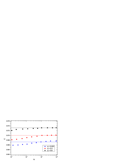
Figure 5: The clustering coefficient of the whole network as a function of the size of the network for various $q$. Results are averaged over ten network realizations for each datum.

After $t$ generation evolutions, the average clustering coefficient $\bar{C}_{t}$ of network $EW(t)$ is given by

$$\bar{C}_{t}=\frac{1}{N_{t}}\sum_{r=0}^{t}\left[\left(\frac{4}{K_{r}}-\frac{1}{K_{r}-1}\right)L_{v}(r)\right],$$ (10)

where the sum runs over all the nodes and $K_{r}$ is the degree of those nodes created at step $r$, which is given by Eq. (4). In the infinite network order limit ($N_{t}\rightarrow\infty$), Eq. (10) converges to a nonzero value $C$, see Fig. 5. Moreover, it can be easily proved that both $\bar{C}_{t}$ and $C$ increase with $q$. Exactly analytical computation shows: when $q$ increases from $0$ to $1$, $C$ grows from $0.5674$ [8] to $0.5745$ [7]. Therefore, the evolutionary networks are highly clustered. Figure 6 shows the average clustering coefficient of the network as a function of $q$, which is in accordance with our above conclusions. From Figs. 4 and 6, one can see that both degree exponent $\gamma$ and clustering coefficient $C$ depend on the parameter $q$. The mechanism resulting in this relation deserves further study. The fact that a biased choice of the active triangles at each iteration may be a possible explanation, see Ref. [13].

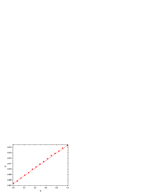
Figure 6: The dependence of the average clustering coefficient on parameter $q$.

4.3 Average path length

From above discussions, one knows that the existing model shows both the scale-free nature and the high clustering at the same time. In fact, our model also possesses small-world property. Next, we will show that our networks have at most a logarithmic average path length (APL) with the number of nodes, where APL means the minimum number of edges connecting a pair of nodes, averaged over all couples of nodes.

Using a mean-field approach similar to that presented in Refs. [14, 15], one can predict the APL of our networks analytically. By construction, at each time step, the number of newly-created nodes is different. In order to distinguish different nodes, we construct a node sequence in the following way: when $\Delta N$ nodes are added at a given time step, we label them as $M+1,M+2,\ldots,M+\Delta N$, where $M$ is the total number of the pre-existing nodes. Eventually, every node is labeled by a unique integer, and the total number of nodes is $N_{t}=\frac{3(1+2q)^{t}+3}{2}$ at time $t$. We denote $L(N)$ as the APL of the ESNs with order $N$. It follows that $L(N)=\frac{2D(N)}{N(N-1)}$, where $D(N)=\sum_{1\leq i\leq j\leq N}d_{i,j}$ is the total distance, and where $d_{i,j}$ is the smallest distance between node $i$ and node $j$. Note that the distances between existing node pairs are not affected by the addition of new nodes. As in the analysis of [14, 15], we can easily derive that $D(N)\sim N^{2}$ in the infinite limit of $N$. Then, $L(N)\sim\ln N$. Thus, there is a slow growth of the APL with the network order $N$. This logarithmic scaling of $L(N)$ with network order $N$, together with the large clustering coefficient obtained in the preceding subsection, shows that the considered graphs have a small-world effect.

In particular, in the case of $q=1$, we can exactly compute the average path length. A previously reported analytical result has shown that the APL for this special case grows logarithmically with the order of the network [7]. In Fig. 7, we report the simulation results on the APL of ESNs for different $q$. From Fig. 7, one can see that APL decreases with increasing $q$. For all $q$, APL increases logarithmically with network order.

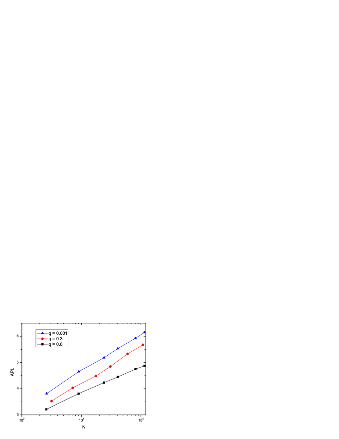
Figure 7: Semilogarithmic graph of the APL versus the network order $N$.

5 Prisoner’s Dilemma game on two limiting cases for ESN

The ultimate goal of study of network structure is to study and understand the workings of systems built upon those networks [3, 4]. Recently, some researchers have focused on the analysis of functional or dynamical aspects of processes occurring on networks. One particular issue attracting much attention is using evolutionary game theory to analyze the evolution of cooperation on different types of networks [16]. Cooperation is ubiquitous in the real-life systems, ranging from biological systems to economic and social systems [17]. Understanding the emergence and survival of cooperative behavior in these systems has become a fundamental and central issue.

After studying the relevant characteristics of network structure, which is described in the previous section, we will study the evolutionary game behavior on the networks, with focus on the game of prisoner’s dilemma (PD). In the simple, one-shot PD game, both receive $R$ under mutual cooperation and $P$ under mutual defection, while a defector exploiting a cooperator gets amount $T$ and the exploited cooperator receives $S$, such that $T>R>P>S$. As a result, it is better to defect regardless of the opponent’s decision, which in turns makes cooperators unable to resist invasion by defectors, and the defection is the only evolutionary stable strategy in fully mixed populations.

We now investigate the evolutionary PD game on our networks to reveal the influences of topological properties on cooperation behavior. Here we only study two limiting cases: $q=1$ and $q\rightarrow 0$ (but $q\neq 0$). As usual in the studies [18, 19], we choose the payoffs as $R=1$, $P=S=0$, and $T=b>1$, and implement the finite population analogue of replicator dynamics. During each generation, each individual $i$ plays the single given game with all its neighbors, and their accumulated payoff being stored in $P_{i}$. After each round of the game, the individual $i$ is allowed to update its strategy by selecting at random a neighbor among all its neighbors, $j$, and comparing their respective payoffs $P_{i}$ and $P_{j}$. If $P_{i}>P_{j}$ , the individual $i$ will keep the same strategy for the next generation. On the contrary, the individual $i$ will adopt the strategy of its neighbor $j$ with a probability dependent on the payoff difference ($P_{j}-P_{i}$) as $\prod_{i\rightarrow j}=(P_{j}-P_{i})/\max\{k_{i},k_{j}\}b$. All individuals update its strategies synchronously during the evolution process.

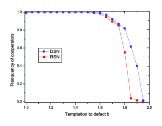
Figure 8: Frequency of cooperators as a function of the temptation to defect $b$.

In Fig. 8, we report the simulated results (i.e. the dependence of the equilibrium frequency of cooperators on the temptation to defect $b$) for both DSN and RSN. Simulations are performed for both networks with order $9843$. Each data point is obtained by averaging over 100 simulations for each of ten different network realizations. From Fig. 8, one can see that for $b<1.6$ the cooperators in the deterministic Sierpinski network is dominant over defectors. And similar phenomenon is also observed for its corresponding random version. Thus, both of the network structures are in favor of cooperation upon defection for a wide range of $b$. Figure 8 also shows that in both networks the frequency of cooperators makes a steady decrease when the temptation changes from $1.6$ to $1.75$, and then drops dramatically when the temptation increases to $2$. On the other hand, for large $b$ (such as $b>1.6$), the equilibrium frequency of DSN is higher than that in RSN, and this phenomenon is more obvious when the temptation is larger and goes up to $2$.

The observed phenomena in Fig. 8 can be explained according to the underlying network structures. Since both DSN and RSN are scale-free networks, this heterogeneous network architecture makes cooperation become the dominating trait over a wide range of temptation to defect $b$ [19, 20]. Although both networks have scale-free property, DSN is more heterogeneous than RSN since the former has a smaller exponent of power-law degree distribution than the latter; at the same time, the average clustering coefficient of DSN is larger than that of RSN. These two different characteristics between DSN and RSN can account for the dissimilar cooperation behavior in both networks [19, 21]: A higher value of average clustering coefficient, together with a smaller exponent of power-law degree distribution, produces an overall improvement of cooperation in DSN, even for a very large temptation to defect, which is compared to that in RSN.

6 Conclusions

In summary, on the basis of Sierpinski gasket, we have proposed and studied one kind of evolving network: evolutionary Sierpinski networks (ESNs). According to the network construction process we have presented an algorithm to generate the networks, based on which we have obtained the analytical and numerical results for degree distribution, clustering coefficient, as well as average path length, which agree well with a large amount of real observations. The degree exponent can be adjusted continuously between $1+\frac{\ln 3}{\ln 2}$ and 3, and the clustering coefficient is very large. Moreover, we have studied the evolutionary PD game on two limiting cases of the ESN.

It should be stressed that the network representation introduced here is convenient for studying the complexity of some real systems and may have wider applicability. For instance, a similar recipe has been recently adopted for investigating the navigational complexity of cities [22]; on the other hand, it is frequently used in RNA folding research [23, 24]; moreover, earlier links associating this network representation with polymers have proven useful to the study of polymer physics [25, 26]. Thus, our study provides a paradigm of representation for the complexity of many real-life systems, making it possible to study the complexity of these systems within the framework of network theory.

Because of its three important properties: power-law degree distribution, small intervertex separation, and large clustering coefficient, the proposed networks possess good structural features in accordance with a variety of real-life networks. Additionally, our networks are maximal planar graphs, which may be helpful for designing printed circuits [11]. Finally, it should be mentioned that although our model can reproduce a few topological characteristics of real-life systems, it remains unknown whether the model can capture a true underlying mechanism responsible for those properties observed in real networks. This belongs to the issue of model evaluation, which is beyond the scope of the present paper but deserves further study in future [27].

Acknowledgment

We thank Yichao Zhang for preparing this manuscript. This research was supported by the National Basic Research Program of China under grant No. 2007CB310806, the National Natural Science Foundation of China under Grant Nos. 60704044, 60873040 and 60873070, Shanghai Leading Academic Discipline Project No. B114, and the Program for New Century Excellent Talents in University of China (NCET-06-0376).

References

- [1] R. Albert and A.-L. Barabási, Rev. Mod. Phys. 74, 47 (2002).
- [2] S.N. Dorogovtsev and J.F.F. Mendes, Adv. Phys. 51, 1079 (2002).
- [3] M.E.J. Newman, SIAM Rev. 45, 167 (2003).
- [4] S. Boccaletti, V. Latora, Y. Moreno, M. Chavez and D.-U. Hwanga, Phys. Rep. 424, 175 (2006).
- [5] A.-L. Barabási and R. Albert, Science 286, 509 (1999).
- [6] D.J. Watts and H. Strogatz, Nature (London) 393, 440 (1998).
- [7] Z. Z. Zhang, S. G. Zhou, T. Zou, L. C. Chen, and J. H. Guan, Eur. Phys. J. B 60, 259 (2007).
- [8] Z. Z. Zhang, S. G. Zhou, Z. Su, T. Zou, and J. H. Guan, Eur. Phys. J. B 65, 141 (2008).
- [9] W. Sierpinski, Comptes Rendus (Paris) 160, 302 (1915).
- [10] C. A. Reiter, Comput. Graphics 18, 885 (1994).
- [11] D.B. West, Introduction to Graph Theory (Prentice-Hall, Upper Saddle River, NJ, 2001).
- [12] E. Ravasz, A.-L. Barabási, Phys. Rev. E 67, 026112 (2003).
- [13] F. Comellas, H. D. Rozenfeld, D. ben-Avraham, Phys. Rev. E 72, 046142 (2005).
- [14] Z. Z. Zhang, L. L. Rong, and F. Comellas, Physica A 364, 610 (2006).
- [15] L. Wang, H. P. Dai, and Y. X. Sun, J. Phys. A: Math. Thero. 40, 13279 (2007).
- [16] G. Szabó and G. Fáth, Phy. Rep. 446, 97 (2007).
- [17] L. A. Dugatkin, Cooperation Among Animals: An Evolutionary Perspective (Oxford University Press, Oxford, 1997).
- [18] M. Nowak and R. May, Nature (London) 359, 826 (1992).
- [19] F. C. Santos and J. M. Pacheco, Phys. Rev. Lett. 95, 098104 (2005).
- [20] J. Gomez-Gardenes, M. Campillo, L. M. Floria, and Y. Moreno, Phys. Rev. Lett. 98, 108103 (2007).
- [21] S. Assenza, J. Gómez-Gardeñes, and V. Latora, Phys. Rev. E 78, 017107 (2008).
- [22] M. Rosvall, A. Trusina, P. Minnhagen, and K. Sneppen, Phys. Rev. Lett. 94, 028701 (2005)
- [23] C. Haslinger and P.F. Stadler, Bull. Math. Biol. 61, 437 (1999).
- [24] A. Kabakçıoğlu and A.L. Stella, Phys. Rev. E 70, 011802 (2004).
- [25] M. Vendruscolo, B. Subramanian, I. Kanter, E. Domany, and J. Lebowitz, Phys. Rev. E 59, 977 (1999).
- [26] A. Kabakçıoğlu and A.L. Stella, Phys. Rev. E 72, 055102(R) (2005).
- [27] A. Cami, N. Deo, Networks, 51, 211 (2008).