Analysis of Fully Discrete Finite Element Methods for a System of Differential Equations Modeling Swelling Dynamics of Polymer Gels

Abstract

The primary goal of this paper is to develop and analyze some fully discrete finite element methods for a displacement-pressure model modeling swelling dynamics of polymer gels under mechanical constraints. In the model, the swelling dynamics is governed by the solvent permeation and the elastic interaction; the permeation is described by a pressure equation for the solvent, and the elastic interaction is described by displacement equations for the solid network of the gel. The elasticity is of long range nature and gives effects for the solvent diffusion. It is the fluid-solid interaction in the gel network drives the system and makes the problem interesting and difficult. By introducing an “elastic pressure” (or “volume change function”) we first present a reformulation of the original model, we then propose a time-stepping scheme which decouples the PDE system at each time step into two sub-problems, one of which is a generalized Stokes problem for the displacement vector field (of the solid network of the gel) and another is a diffusion problem for a “pseudo-pressure” field (of the solvent of the gel). To make such a multiphysical approach feasible, it is vital to find admissible constraints to resolve the uniqueness issue for the generalized Stokes problem and to construct a “good” boundary condition for the diffusion equation so that it also becomes uniquely solvable. The key to the first difficulty is to discover certain conservation laws (or conserved quantities) for the PDE solution of the original model, and the solution to the second difficulty is to use the generalized Stokes problem to generate a boundary condition for the diffusion problem. This then lays down the theoretical foundation for one to utilize any convergent Stokes solver (and its code) together with any convergent diffusion equation solver (and its code) to solve the polymer gel model. In the paper, the Taylor-Hood mixed finite element method combined with the continuous linear finite element method are chosen as an example to present the ideas and to demonstrate the viability of the proposed multiphysical approach. It is proved that, under a mesh constraint, both the proposed semi-discrete (in space) and fully discrete methods enjoy some discrete energy laws which mimic the differential energy law satisfied by the PDE solution. Optimal order error estimates in various norms are established for the numerical solutions of both the semi-discrete and fully discrete methods. Numerical experiments are also presented to show the efficiency of the proposed approach and methods.

1 Introduction

A gel is a soft poroelastic material which consists of a solid network and a colloidal solvent. The solid network spans the volume of the solvent medium. The solvent can permeate through the solid network and the permeation can be controlled by external forces. Both by weight and volume, gels are mostly liquid in composition and thus exhibit densities similar to liquids. However, they have the structural coherence of a solid and can be deformed. A gel network can be composed of a wide variety of materials, including particles, polymers and proteins, which then gives different types gels such hydrogels, organogels and xerogels (cf. [9, 13]). Gels have some fascinating properties, in particular, they display thixotropy which means that they become fluid when agitated, but resolidify when resting. In general, gels are apparently solid, jelly-like materials, they exhibit an important state of matter found in a wide variety of biomedical and chemical systems (cf. [9, 10, 19, 20] and the references therein).

This paper develops and analyzes some fully discrete finite element methods for a displacement-pressure model for polymer gels. The model, which was proposed by M. Doi et al in [9, 19, 20], describes swelling dynamics of polymer gels (under mechanical constraints). Let $\Omega\subset\mathbb{R}^{d}\,(d=1,2,3)$ be a bounded domain and denote the initial region occupied by the gel. Let $\mathbf{u}(x,t)$ denote the displacement of the gel at the point $x\in\Omega$ in the space and at the time $t$, $\mathbf{v}_{s}(x,t)$ and $p(x,t)$ be the velocity and the pressure of the solvent at $(x,t)$. Following [9], the governing equation for the swelling dynamics of polymer gels are given by

(1) $${\mbox{\rm div\,}}\bigl{(}\sigma(\mathbf{u})-pI\bigr{)} =0,$$

(2) $$\xi(\mathbf{v}_{s}-\mathbf{u}_{t}) =-(1-\phi)\nabla p,$$

(3) $${\mbox{\rm div\,}}\bigl{(}\phi\mathbf{u}_{t}+(1-\phi)\mathbf{v}_{s}\bigr{)} =0.$$

Here $\xi$ is the friction constant associated with the motion of the polymer relative to the solvent, $\phi$ is the volume fraction of the polymer, $I$ denotes the $d\times d$ identity matrix, and $\sigma(\mathbf{u})$ stands for the stress tensor of the gel network, which is given by a constitutive equation. In this paper, we use the following linearized form of the stress tensor:

(4) $$\sigma(\mathbf{u}):=\bigl{(}K-\frac{2}{3}G\bigr{)}{\mbox{\rm div\,}}\mathbf{u}\,I+2G\,\varepsilon(\mathbf{u}),\qquad\varepsilon(\mathbf{u}):=\frac{1}{2}\bigl{(}\nabla\mathbf{u}+\nabla\mathbf{u}^{T}\bigr{)},$$

where $K$ and $G$ are respectively the bulk and shear modulus of the gel (cf. [9, 7]). We remark that (1) stands for the force balance, (2) states Darcy’s law for the permeation of solvent through the gel network, and (3) describes the incompressibility condition. In addition, if we introduce the total stress $\widetilde{\sigma}(\mathbf{u},p):=\sigma(\mathbf{u})-pI$, then equation (1) becomes ${\mbox{\rm div\,}}\widetilde{\sigma}(\mathbf{u},p)=0$.

Substituting (4) into (1) and (2) into (3) yield the following basic equations for swelling dynamics of polymer gels (see [19])

(5) $$\alpha\nabla{\mbox{\rm div\,}}\mathbf{u}+\beta\Delta\mathbf{u} =\nabla p, \qquad\alpha:=K+\frac{G}{3},\quad\beta:=G,$$

(6) $${\mbox{\rm div\,}}\mathbf{u}_{t} =\kappa\Delta p, \qquad\kappa:=\frac{(1-\phi)^{2}}{\xi},$$

which hold in the space-time domain $\Omega_{T}:=\Omega\times(0,T)$ for some given $T>0$.

To close the above system, we need to prescribe boundary and initial conditions. Only one initial condition is required for the system, which is

(7) $$\mathbf{u}(\cdot,0)=\mathbf{u}_{0}(\cdot)\qquad\mbox{in }\Omega.$$

Various sets of boundary conditions are possible and each of them describes a certain type mechanical condition and solvent permeation condition (cf. [19, 20]). In this paper we consider the following set of boundary conditions

(8) $$(\sigma(\mathbf{u})-pI)\nu=\mathbf{f},\qquad\frac{{\partial}p}{{\partial}\nu}=0\quad\mbox{on }\Omega_{T}:={\partial}\Omega\times(0,T),$$

where $\nu$ denotes the outward normal to ${\partial}\Omega$. (8)₁ means that the mechanical force $\mathbf{f}$ is applied on the boundary of the gel. Since $\frac{{\partial}p}{{\partial}\nu}=(\mathbf{v}_{s}-\mathbf{u}_{t})\cdot\nu$, hence, (8)₂ implies that the solvent can not permeate through the gel boundary. We also remark that the force function $\mathbf{f}$ must satisfy the compatibility condition

$$\int_{{\partial}\Omega}\mathbf{f}\,dS=0.$$

Problem (5)–(8) is interesting and difficult due to its multiphysical nature which describes the complicate fluid and solid interaction inside the gel network. It is numerically tricky to solve because it is difficult to design a good and workable time-stepping scheme. For example, one natural attempt would be at each time step first to solve a Poisson problem for $p$ and then to solve a linear elasticity problem for $\mathbf{u}$. However, this strategy is difficult to realize because there is no good way to compute the source term ${\mbox{\rm div\,}}\mathbf{u}_{t}$ for the Poisson equation. In fact, the strategy even has a difficulty to start due to the fact that no initial condition is provided for the pressure $p$.

To overcome the difficulty, in this paper we shall use a reformulation of system (5)–(6), which is now introduced. Define

(9) $$q:={\mbox{\rm div\,}}\mathbf{u}.$$

Physically, $q$ measures the volume change of the solid network of the gel, and often called “elastic pressure” or “volume change function”. Taking divergence on (5) yields

$$(\alpha+\beta)\Delta q=\Delta p,$$

which and (6) imply that $q$ satisfies the following diffusion equation

(10) $$q_{t}=D\Delta q,\qquad D:=\kappa\bigl{(}K+\frac{4}{3}G\bigr{)}.$$

However, the usefulness of the above diffusion equation is hampered by the lack of boundary condition for $q$. We like to note that the above diffusion equation for $q$ was first noticed by M. Doi [8], but it was not utilized before exactly because of the lack of boundary condition for $q$. Nevertheless, using the new variable $q$ we can rewrite (5)–(6) as

(11) $$\beta\Delta\mathbf{u} =\nabla\widetilde{p}, \qquad\widetilde{p}:=p-\alpha q,$$

(12) $${\mbox{\rm div\,}}\mathbf{u} =q,$$

(13) $$q_{t} =\kappa\Delta p, \qquad p=\widetilde{p}+\alpha q.$$

An immediate consequence of the above reformulation is that (11)-(12) implies $(\mathbf{u},\widetilde{p})$ satisfies the generalized Stokes equations with $q$ being the source term at each time $t$, and $q$ satisfies a diffusion equation and it interacts with $(\mathbf{u},\widetilde{p})$ only at the boundary ${\partial}\Omega$.

This is a key observation because it not only reveals the underlying physical process of swelling dynamics of the gel, but also gives the “right” hint on how the problem should be solved numerically. This indeed motivates the main idea of this paper, that is, at each time step, we first solve the generalized Stokes problem for $(\mathbf{u},\widetilde{p})$, which in turn provides (implicitly) an updated boundary condition for $q$, we then use this new boundary condition to solve the diffusion equation for $q$. The process is repeated iteratively until the final time step is reached. However, in order to make this idea work, there is one crucial issue needs to be addressed. That is, for a given $q$ the generalized Stokes problem for $(\mathbf{u},\widetilde{p})$ is only unique up to additive constants. Clearly, how to correctly enforce the uniqueness of the generalized Stokes problem is the bottleneck of this approach. It is easy to understand that one can not use arbitrary constraints to fix $(\mathbf{u},\widetilde{p})$ because this will lead to bad or even divergent numerical schemes if the exact PDE solution does not satisfy the constraints. Instead, the constraints which can be used to fix $(\mathbf{u},\widetilde{p})$ should be those satisfied by the exact solution of the PDE system. To the end, we need to discover some invariant (or conserved) quantities for the exact PDE solution. It turns out that the situation is precisely what we anticipated and wanted. We are able to show that the exact PDE solution $(\mathbf{u},p,\widetilde{p},q)$ satisfies the following identities (see Section 2 below for a proof):

(14) $$\int_{\Omega}q(x,t)dx \equiv C_{q}:=\int_{\Omega}q_{0}(x)dx:=\int_{\Omega}{\mbox{\rm div\,}}\mathbf{u}_{0}(x)dx,$$

(15) $$\int_{\Omega}p(x,t)dx \equiv C_{p}:=c_{d}C_{q}-\frac{1}{d}\int_{{\partial}\Omega}\mathbf{f}(x,t)\cdot x\,dS,$$

(16) $$\int_{{\partial}\Omega}\mathbf{u}(x,t)\cdot\nu\,dS \equiv C_{\mathbf{u}}:=\int_{{\partial}\Omega}\mathbf{u}_{0}(x)\cdot\nu\,dS=C_{q},$$

where $d$ denote the dimension of $\Omega$ and

(17) $$c_{d}:=\alpha+\frac{\beta}{d}=\begin{cases}K+\frac{5G}{6}&\quad\mbox{if }d=2,\\ K+\frac{2G}{3}&\quad\mbox{if }d=3.\end{cases}$$

Obviously, the right-hand sides of (14) and (16) are constants. The right-hand side of (15) is also a constant provided that $\mathbf{f}$ is independent of $t$, otherwise, it is a known function of $t$. In this paper, we shall only consider the case that $\mathbf{f}$ is independent of $t$. It follows from (14) and (15) that

(18) $$\int_{\Omega}\widetilde{p}(x,t)dx\equiv C_{\widetilde{p}}:=C_{p}-\alpha C_{q}=\frac{\beta C_{q}}{d}-\frac{1}{d}\int_{{\partial}\Omega}\mathbf{f}(x)\cdot x\,dS.$$

It is clear now that (18) and (16) provide two natural conditions which can be used to uniquely determine the solution $(\mathbf{u},\widetilde{p})$ to the generalized Stokes problem (11)–(12) for a given source term $q$. This then leads to the following time-discretization for problem (5)–(8):

Algorithm 1:

• Set $q^{0}=q_{0}:={\mbox{\rm div\,}}\mathbf{u}_{0}$ and $\mathbf{u}^{0}:=\mathbf{u}_{0}$.

• For $n=0,1,2,\cdots$, do the following two steps

  Step 1: Solve for $(\mathbf{u}^{n+1},\widetilde{p}^{n+1})$ such that

  (19) $$-\beta\Delta\mathbf{u}^{n+1}+\nabla\widetilde{p}^{n+1} =0,\quad \qquad\mbox{in }\Omega_{T},$$

  (20) $${\mbox{\rm div\,}}\mathbf{u}^{n+1} =q^{n} \qquad\mbox{in }\Omega_{T},$$

  (21) $$\beta\frac{{\partial}\mathbf{u}^{n+1}}{{\partial}\nu}-\widetilde{p}^{n+1}\nu =\mathbf{f} \qquad\mbox{on }{\partial}\Omega_{T},$$

  (22) $$(\widetilde{p}^{n+1},1)=C_{\widetilde{p}},\quad\langle\mathbf{u}^{n+1},\nu\rangle =C_{\mathbf{u}}.$$

  Step 2: Solve for $q^{n+1}$ such that

  (23) $$d_{t}q^{n+1}-\kappa\Delta(\alpha q^{n+1}+\widetilde{p}^{n+1}) =0, \qquad\mbox{in }\Omega_{T},$$

  (24) $$\alpha\frac{{\partial}q^{n+1}}{{\partial}\nu} =-\frac{{\partial}\widetilde{p}^{n+1}}{{\partial}\nu} \qquad\mbox{on }{\partial}\Omega_{T},$$

  (25) $$(q^{n+1},1) =C_{q},$$

  where $d_{t}q^{n+1}:=(q^{n+1}-q^{n})/{\Delta t}$.

We note that (23) is the implicit Euler scheme, which is chosen just for the ease of presentation, it can be replaced by other time-stepping schemes. (24) provides a Neumann boundary condition for $q^{n+1}$. Another subtle issue is the role which the initial value $\mathbf{u}_{0}$ plays in the algorithm. Seems $\mathbf{u}_{0}$ is only needed to produce $q_{0}$ and there is no need to have $\mathbf{u}^{0}$ in order to execute the algorithm. However, to ensure the stability and convergence of the algorithm, it turns out that $\mathbf{u}^{0}$ not only needs to be provided but also must be carefully constructed when the algorithm is discretized (see Sections 3 and 4).

The above algorithm has a couple attractive features. First, it is easy to use. Second, it allows one to make use of any available numerical methods (finite element, finite difference, finite volume, spectral and discontinuous Galerkin) and computer codes for the Stokes problem and the Poisson problem to solve the gel swelling dynamics model (5)–(8). We remark that an almost same model as (5)–(8) also arise from different applications in poroelasticity and soil mechanics and are known as Boit’s consolidation model (cf. [2, 14] and the references therein). [14] proposed and analyzed a standard finite element method which directly approximates $(\mathbf{u},p)$ under the (restrictive) divergence-free assumption on the initial condition $\mathbf{u}_{0}$.

This paper consists of four additional sections. In Section 2, we first introduce notation used in this paper. We then present a PDE analysis for the gel swelling dynamics model (5)–(8), which includes deriving a dissipative energy law, establishing existence and uniqueness, and in particular, proving the conservation laws stated in (14)–(16) and (18). In Section 3, we first propose a semi-discrete (in space) finite element discretization for problem (5)–(8) based on the multiphysical reformulation (11)–(13). The well-known Taylor-Hood mixed element and the $P_{1}$ conforming finite element are used as an example to present the ideas. It is proved that the solution of the semi-discrete method satisfies a discrete energy law which mimics the differential energy law enjoyed by the PDE solution, and the semi-discrete numerical solution also satisfies the conservation laws (14)–(16) and (18). We then derive optimal order error estimates in various norms for the semi-discrete numerical solution. In Section 4, fully discrete finite element methods are constructed by combining the time-stepping scheme of Algorithm $1$ and the semi-discrete finite element methods of Section 3. The main results of this section include proving a fully discrete energy law for the numerical solution and establishing optimal order error estimates for the fully discrete finite element methods. Finally, in Section 5, we present some numerical experiments to gauge the efficiency of the proposed approach and methods.

2 PDE analysis for problem (5)–(8)

The standard Sobolev space notation is used in this paper, we refer to [4, 6, 18] for their precise definitions. In particular, $(\cdot,\cdot)$ and $\langle\cdot,\cdot\rangle$ denote respectively the standard $L^{2}(\Omega)$ and $L^{2}({\partial}\Omega)$ inner products. For any Banach space $B$, we let $\mathbf{B}=[B]^{d}$ and use ${\mathbf{B}}^{\prime}$ to denote its dual space. In particular, we use $(\cdot,\cdot)_{\small\rm dual}$ and $\langle\cdot,\cdot\rangle_{\small\rm dual}$ to denote the dual products on $(H^{1}(\Omega))^{\prime}\times H^{1}(\Omega)$ and $\mathbf{H}^{-\frac{1}{2}}({\partial}\Omega)\times\mathbf{H}^{\frac{1}{2}}({\partial}\Omega)$, respectively. $\|\,\cdot\,\|_{L^{p}(B)}$ is a shorthand notation for $\|\,\cdot\,\|_{L^{p}((0,T);B)}$.

We also introduce the function spaces

$$L^{2}_{0}(\Omega):=\{q\in L^{2}(\Omega);\,(q,1)=0\},\qquad\mathbf{X}:=\{\mathbf{v}\in\mathbf{H}^{1}(\Omega);\,\langle\mathbf{v},\nu\rangle=0\}.$$

It is well known [18] that the following so-called inf-sup condition holds in the space $\mathbf{X}\times L^{2}_{0}(\Omega)$:

(26) $$\sup_{\mathbf{v}\in\mathbf{X}}\frac{({\mbox{\rm div\,}}\mathbf{v},\varphi)}{\|\,\nabla\mathbf{v}\,\|_{L^{2}}}\geq\alpha_{0}\|\,\varphi\,\|_{L^{2}}\qquad\forall\varphi\in L^{2}_{0}(\Omega),\quad\alpha_{0}>0.$$

Throughout the paper, we assume $\Omega\subset\mathbb{R}^{d}$ be a bounded polygonal domain such that $\Delta:H^{1}_{0}(\Omega)\cap H^{2}(\Omega)\rightarrow L^{2}(\Omega)$ is an isomorphism; see  [11, 12]. In addition, $C$ is used to denote a generic positive constant which is independent of $\mathbf{u},\,p,\,\widetilde{p},\,q$, and the mesh parameters $h$ and $\Delta t$.

We now give a definition of weak solutions to (5)-(8).

Definition 1.

Let $(\mathbf{u}_{0},\mathbf{f})\in\mathbf{H}^{1}(\Omega)\times\mathbf{H}^{-\frac{1}{2}}({\partial}\Omega)$, and $\langle\mathbf{f},1\rangle_{\small\rm dual}=0$. Given $T>0$, a tuple $(\mathbf{u},p)$ with

$$\mathbf{u}\in L^{\infty}\bigl{(}0,T;\mathbf{H}^{1}(\Omega)),\quad{\mbox{\rm div\,}}\mathbf{u}\in H^{1}(0,T;H^{-1}(\Omega)),\quad p\in L^{2}\bigl{(}0,T;H^{1}(\Omega)\bigr{)},$$

is called a weak solution to (5)–(8), if there hold for almost every $t\in[0,T]$

(27) $$\bigl{(}({\mbox{\rm div\,}}\mathbf{u})_{t},\varphi\bigr{)}_{\small\rm dual}+\kappa\bigl{(}\nabla p,\nabla\varphi\bigr{)} =0 \quad\forall\varphi\in H^{1}(\Omega),$$

(28) $$\alpha\bigl{(}{\mbox{\rm div\,}}\mathbf{u},{\mbox{\rm div\,}}\mathbf{v}\bigr{)}+\beta\bigl{(}\nabla\mathbf{u},\nabla\mathbf{v}\bigr{)}-\bigl{(}p,{\mbox{\rm div\,}}\mathbf{v}\bigr{)} =\langle\mathbf{f},\mathbf{v}\rangle_{\small\rm dual} \quad\forall\mathbf{v}\in\mathbf{H}^{1}(\Omega),$$

(29) $$\mathbf{u}(0) =\mathbf{u}_{0}.$$

Similarly, we define weak solutions to problem (11)-(13), (7)-(8).

Definition 2.

Let $(\mathbf{u}_{0},\mathbf{f})\in\mathbf{H}^{1}(\Omega)\times\mathbf{H}^{-\frac{1}{2}}({\partial}\Omega)$, and $\langle\mathbf{f},1\rangle_{\small\rm dual}=0$. Given $T>0$, a triple $(\mathbf{u},\widetilde{p},q)$ with

$$\mathbf{u}\in L^{\infty}\bigl{(}0,T;\mathbf{H}^{1}(\Omega)), \qquad\widetilde{p}\in L^{2}\bigl{(}0,T;L^{2}(\Omega)\bigr{)},$$

$$q\in L^{\infty}(0,T;L^{2}(\Omega))\cap H^{1}\bigl{(}0,T;H^{-1}(\Omega)\bigr{)}, \qquad\alpha q+\widetilde{p}\in L^{2}(0,T;H^{1}(\Omega)),$$

is called a weak solution to (11)–(13), (7)-(8) if there hold for almost every $t\in[0,T]$

(30) $$\beta\bigl{(}\nabla\mathbf{u},\nabla\mathbf{v}\bigr{)}-\bigl{(}\widetilde{p},{\mbox{\rm div\,}}\mathbf{v}\bigr{)} =\langle\mathbf{f},\mathbf{v}\rangle_{\small\rm dual} \quad\forall\mathbf{v}\in\mathbf{H}^{1}(\Omega),$$

(31) $$\bigl{(}{\mbox{\rm div\,}}\mathbf{u},\varphi\bigr{)} =\bigl{(}q,\varphi\bigr{)} \quad\forall\varphi\in L^{2}(\Omega),$$

(32) $$\mathbf{u}(0) =\mathbf{u}_{0},$$

(33) $$\bigl{(}q_{t},\psi\bigr{)}_{\small\rm dual}+\kappa\bigl{(}\nabla(\alpha q+\widetilde{p}),\nabla\psi\bigr{)} =0 \quad\forall\psi\in H^{1}(\Omega),$$

(34) $$q(0) =q_{0}:={\mbox{\rm div\,}}\mathbf{u}_{0}.$$

Remark 2.1.

(a) Clearly, $p:=\alpha q+\widetilde{p}$ gives back the pressure in the original formulation. What interesting is that both $q$ and $\widetilde{p}$ are only $L^{2}$-functions in the spatial variable but their combination $\alpha q+\widetilde{p}$ is an $H^{1}$-function. In other words, the new formulation provides an $L^{2}-L^{2}$ decomposition for the pressure $p$. It turns out that this decomposition will have a significant numerical impact because it allows one to use low order (hence cheap) finite elements to approximate $q$ and $\widetilde{p}$ but still to be able to approximate the pressure $p$ with high accuracy.

(b) (33) implicitly imposes the following boundary condition for $q$:

(35) $$\alpha\frac{{\partial}q}{{\partial}\nu}=-\frac{{\partial}\widetilde{p}}{{\partial}\nu}\qquad\mbox{on }{\partial}\Omega.$$

Since problem (27)–(29) consists of two linear equations, its solvability should follows easily if we can establish a priori energy estimates for its solutions. The following dissipative energy law just serves that purpose.

Lemma 3.

Every weak solution $(\mathbf{u},p)$ of problem (5)–(8) satisfies the following energy law:

(36) $$E(t)+\kappa\int_{0}^{t}\|\,\nabla p(s)\,\|_{L^{2}}^{2}\,ds=E(0)\qquad\forall t\in(0,T],$$

where

$$E(t):=\frac{1}{2}\Bigl{[}\beta\|\,\nabla\mathbf{u}(t)\,\|_{L^{2}}^{2}+\alpha\|\,{\mbox{\rm div\,}}\mathbf{u}(t)\,\|_{L^{2}}^{2}-2\langle\mathbf{f},\mathbf{u}(t)\rangle_{\small\rm dual}\Bigr{]}.$$

Moreover,

(37) $$\|\,({\mbox{\rm div\,}}\mathbf{u})_{t}\,\|_{L^{2}(H^{-1})}=\kappa\|\,\Delta p\,\|_{L^{2}(H^{-1})}\leq E(0)^{\frac{1}{2}}.$$

Proof.

We first consider the case $\mathbf{u}\in H^{1}(0,T;\mathbf{H}^{1}(\Omega))$. Setting $\varphi=p$ in (27) and $\mathbf{v}=\mathbf{u}_{t}$ in (28) yield

$$\bigl{(}{\mbox{\rm div\,}}\mathbf{u}_{t}(t),p(t)\bigr{)}+\kappa\|\,\nabla p\,\|_{L^{2}}^{2} =0,$$

$$\frac{d}{dt}\Bigl{[}\frac{\alpha}{2}\|\,{\mbox{\rm div\,}}\mathbf{u}(t)\,\|_{L^{2}}^{2}+\frac{\beta}{2}\|\,\nabla\mathbf{u}(t)\,\|_{L^{2}}^{2}\Bigr{]} =\frac{d}{dt}\langle\mathbf{f},\mathbf{u}(t)\rangle_{\small\rm dual}+\bigl{(}p(t),{\mbox{\rm div\,}}\mathbf{u}_{t}(t)\bigr{)}.$$

(36) follows from adding the above two equations and integrating the sum in $t$ over the interval $(0,s)$ for any $s\in(0,T]$.

If $(\mathbf{u},p)$ is only a weak solution, then $\mathbf{u}_{t}$ could not be used as a test function in (28). However, this difficulty can be easily overcome by using $\mathbf{u}^{\delta}_{t}$ as a test function in (28), where $\mathbf{u}^{\delta}$ denotes a mollification of $\mathbf{u}$ through a symmetric mollifier (cf. [11, Chapter 7]), and by passing to the limit $\delta\to 0$.

Finally, (37) follows immediately from (27) and (36). The proof is completed. ∎

Remark 2.2.

Lemma 3 and Theorem 5 can be easily carried over to the reformulated problem (11)–(13), (7)–(8). The only difference is that the energy law (36) now is replaced by the following equivalent energy law:

(38) $$J(t)+\kappa\int_{0}^{t}\|\,\nabla[\widetilde{p}(s)+\alpha q(s)]\,\|_{L^{2}}^{2}\,ds=J(0)\qquad\forall t\in(0,T],$$

and (37) is replaced by

(39) $$\|\,q_{t}\,\|_{L^{2}(H^{-1})}\leq\sqrt{\kappa}\|\,\nabla(\widetilde{p}+\alpha q)\,\|_{L^{2}(L^{2})}\leq J(0)^{\frac{1}{2}}.$$

Where

$$J(t):=\frac{1}{2}\Bigl{[}\beta\|\,\nabla\mathbf{u}(t)\,\|_{L^{2}}^{2}+\alpha\|\,q(t)\,\|_{L^{2}}^{2}-2\langle\mathbf{f},\mathbf{u}(t)\rangle_{\small\rm dual}\Bigr{]}.$$

We also note that the weak solution to problem (11)–(13), (7)–(8) is understood in the sense of Definition 2.

Lemma 4.

Weak solutions of problem (5)–(8) and problem (11)–(13),(7)–(8) satisfy the conservation laws (14)–(16), and (18).

Proof.

(14) and (16) follows immediately from taking $\psi\equiv 1$ in (33), $\varphi\equiv 1$ in both (31) and (27) followed by integrating in $t$ and appealing to the divergence theorem.

To prove (15), taking $\mathbf{v}=x$ in (28) and using the identities $\nabla x=I$ and ${\mbox{\rm div\,}}x=d$ we get

$$\alpha\bigl{(}{\mbox{\rm div\,}}\mathbf{u},d\bigr{)}+\beta\bigl{(}\nabla\mathbf{u},I\bigr{)}-\bigl{(}p,d\bigr{)}=\langle\mathbf{f},x\rangle_{\small\rm dual}$$

Hence,

$$\bigl{(}p,1\bigr{)} =\alpha\bigl{(}{\mbox{\rm div\,}}\mathbf{u},1\bigr{)}+\frac{\beta}{d}\bigl{(}{\mbox{\rm div\,}}\mathbf{u},1\bigr{)}-\frac{1}{d}\langle\mathbf{f},x\rangle_{\small\rm dual}$$

$$=\Bigl{(}\alpha+\frac{\beta}{d}\Bigr{)}\bigl{(}{\mbox{\rm div\,}}\mathbf{u}_{0},1\bigr{)}-\frac{1}{d}\langle\mathbf{f},x\rangle_{\small\rm dual}$$

$$=c_{d}C_{q}-\frac{1}{d}\langle\mathbf{f},x\rangle_{\small\rm dual},$$

where $c_{d}$ and $C_{q}$ are defined in (17) and (14). So we obtain (15).

Similarly, (18) follows by taking $\mathbf{v}=x$ in (30). The proof is complete. ∎

With the help of the above two lemmas, we can show the solvability of problem (5)–(8).

Theorem 5.

Suppose $(\mathbf{u}_{0},\mathbf{f})\in\mathbf{H}^{1}(\Omega)\times\mathbf{H}^{-\frac{1}{2}}({\partial}\Omega)$, and $\langle\mathbf{f},1\rangle_{\small\rm dual}=0$. Then there exists a unique weak solution to (5)–(8) in the sense of Definition 1, and there exists a unique solution to to (11)–(13), (7)–(8).

Proof.

The uniqueness is an immediate consequence of the energy laws (36) and (38) and the conservation laws (14)–(16) and (18).

The existence can be easily proved by using (abstract) Galerkin method and the standard compactness argument (cf. [18]). The energy laws (36) and (38) provide the necessary uniform estimates for the Galerkin approximate solutions. We omit the details because the derivation is standard. ∎

Again, exploiting the linearity of the system, we have the following regularity results for the weak solution.

Theorem 6.

Let $(\mathbf{u},p,\widetilde{p},q)$ be the weak solution of (30)–(34) Then there holds the following estimates:

(40) $$\sqrt{\beta}\|\,\sqrt{t}\nabla\mathbf{u}_{t}\,\|_{L^{2}(L^{2})}+\sqrt{\alpha}\|\,\sqrt{t}q_{t}\,\|_{L^{2}(L^{2})}+\sqrt{\kappa}\|\,\sqrt{t}\nabla p\,\|_{L^{\infty}(L^{2})} \leq J(0)^{\frac{1}{2}}.$$

(41) $$\sqrt{\beta}\|\,t\nabla\mathbf{u}_{t}\,\|_{L^{\infty}(L^{2})}+\sqrt{\alpha}\|\,tq_{t}\,\|_{L^{\infty}(L^{2})}+\sqrt{\kappa}\|\,t\nabla p_{t}\,\|_{L^{2}(L^{2})} \leq[2J(0)]^{\frac{1}{2}}.$$

(42) $$\|\,tq_{tt}\,\|_{L^{2}(H^{-1})} \leq[2J(0)]^{\frac{1}{2}}.$$

(43) $$\kappa\sqrt{\alpha}\|\,\sqrt{t}\Delta p\,\|_{L^{2}(L^{2})}=\sqrt{\alpha}\|\,\sqrt{t}q_{t}\,\|_{L^{2}(L^{2})} \leq J(0)^{\frac{1}{2}}.$$

(44) $$\kappa\sqrt{\alpha}\|\,t\Delta p\,\|_{L^{\infty}(L^{2})}=\sqrt{\alpha}\|\,tq_{t}\,\|_{L^{\infty}(L^{2})} \leq[2J(0)]^{\frac{1}{2}}.$$

(45) $$\|\,\nabla\widetilde{p}\,\|_{L^{2}(L^{2})}+\|\,\nabla\widetilde{p}\,\|_{L^{\infty}(L^{2})}+\alpha\sqrt{\kappa}\|\,\nabla q\,\|_{L^{2}(L^{2})}$$

$$+\alpha\sqrt{\kappa}\|\,\sqrt{t}\nabla q\,\|_{L^{\infty}(L^{2})} \leq C(C_{\widetilde{p}},J(0)).{}$$

(46) $$\beta\|\,\Delta\mathbf{u}\,\|_{L^{\infty}(L^{2})}=\|\,\nabla\widetilde{p}\,\|_{L^{\infty}(L^{2})} \leq C(C_{\widetilde{p}},J(0)).$$

Where $C(T,C_{\widetilde{p}},J(0))$ denotes some positive constant which depends on $T,C_{\widetilde{p}}$ and $J(0)$.

Proof.

Differentiating each of equations (30), (31) and (33) with respect to $t$ yields (note that $\mathbf{f}$ is assumed to be independent of $t$)

(47) $$\beta\bigl{(}\nabla\mathbf{u}_{t},\nabla\mathbf{v}\bigr{)}-\bigl{(}\widetilde{p}_{t},{\mbox{\rm div\,}}\mathbf{v}\bigr{)} =0 \quad\forall\mathbf{v}\in\mathbf{H}^{1}(\Omega),$$

(48) $$\bigl{(}{\mbox{\rm div\,}}\mathbf{u}_{t},\varphi\bigr{)} =\bigl{(}q_{t},\varphi\bigr{)} \quad\forall\varphi\in L^{2}(\Omega),$$

(49) $$\bigl{(}q_{tt},\psi\bigr{)}_{\small\rm dual}+\kappa\bigl{(}\nabla(\alpha q+\widetilde{p})_{t},\nabla\psi\bigr{)} =0 \quad\forall\psi\in H^{1}(\Omega).$$

Taking $\mathbf{v}=t\mathbf{u}_{t}$ in (47), $\varphi=t\widetilde{p}_{t}$ in (48), $\psi=tp_{t}=t(\widetilde{p}+\alpha q)_{t}$ in (33), and adding the resulted equations we get

$$t\beta\|\,\nabla\mathbf{u}_{t}\,\|_{L^{2}}^{2}+t\alpha\|\,q_{t}\,\|_{L^{2}}^{2}+\frac{\kappa}{2}\frac{d}{dt}\Bigl{(}t\|\,\nabla p\,\|_{L^{2}}^{2}\Bigr{)}=\frac{\kappa}{2}\|\,\nabla p\,\|_{L^{2}}^{2}.$$

Integrating in $t$ over $(0,T)$ gives (40).

Alternatively, setting $\mathbf{v}=t^{2}\mathbf{u}_{tt}$ in (47), $\varphi=t^{2}\widetilde{p}_{t}$ in (48) (after differentiating in $t$ one more time), $\psi=t^{2}p_{t}=t^{2}(\widetilde{p}+\alpha q)_{t}$ in (49), and adding the resulted equations we have

$$\frac{1}{2}\frac{d}{dt}\Bigl{[}t^{2}\beta\|\,\nabla\mathbf{u}_{t}\,\|_{L^{2}}^{2}+t^{2}\alpha\|\,q_{t}\,\|_{L^{2}}^{2}\Bigr{]}+t^{2}\kappa\|\,\nabla p_{t}\,\|_{L^{2}}^{2}=t\beta\|\,\nabla\mathbf{u}_{t}\,\|_{L^{2}}^{2}+t\|\,q_{t}\,\|_{L^{2}}^{2}.$$

Integrating in $t$ over $(0,T)$ and using (40) yield (41).

(42)–(44) are immediate consequences of (49), (40), and (41).

Choose $\phi_{0}\in C^{1}(\overline{\Omega})$ such that $(\phi_{0},1)=C_{\widetilde{p}}$. Then $\widetilde{p}-\phi_{0}\in L^{2}_{0}(\Omega)$. By an equivalent version of the inf-sup condition (cf. [1]) we have

$$\|\,\nabla(\widetilde{p}-\phi_{0})\,\|_{L^{2}} \leq\alpha_{0}^{-1}\sup_{\mathbf{v}\in\mathbf{H}_{0}^{1}(\Omega)}\frac{\bigl{(}\nabla(\widetilde{p}-\phi_{0}),\mathbf{v}\bigr{)}}{\|\,\nabla\mathbf{v}\,\|_{L^{2}}}$$

$$\leq\alpha_{0}^{-1}\sup_{\mathbf{v}\in\mathbf{H}_{0}^{1}(\Omega)}\frac{-\beta\bigl{(}\nabla\mathbf{u},\nabla\mathbf{v}\bigr{)}}{\|\,\nabla\mathbf{v}\,\|_{L^{2}}}+\alpha_{0}^{-1}\sqrt{d}\|\,\phi_{0}\,\|_{L^{2}}$$

$$\leq\alpha_{0}^{-1}\Bigl{[}\beta\|\,\nabla\mathbf{u}\,\|_{L^{2}}+\sqrt{d}\|\,\phi_{0}\,\|_{L^{2}}\Bigr{]}.$$

Hence,

$$\|\,\nabla\widetilde{p}\,\|_{L^{2}}\leq\|\,\nabla\phi_{0}\,\|_{L^{2}}+\alpha_{0}^{-1}\Bigl{[}\beta\|\,\nabla\mathbf{u}\,\|_{L^{2}}+\sqrt{d}\|\,\phi_{0}\,\|_{L^{2}}\Bigr{]},$$

which together with (38) and (40) imply that (recall $p=\widetilde{p}+\alpha q$)

$$\|\,\nabla\widetilde{p}\,\|_{L^{2}(L^{2})}\leq\sqrt{T}\|\,\nabla\widetilde{p}\,\|_{L^{\infty}(L^{2})}\leq\sqrt{T}\|\,\nabla\phi_{0}\,\|_{L^{2}}+\alpha_{0}^{-1}\sqrt{T}\Bigl{[}\beta J(0)^{\frac{1}{2}}+\sqrt{d}\|\,\phi_{0}\,\|_{L^{2}}\Bigr{]},$$

$$\alpha\sqrt{\kappa}\|\,\nabla q\,\|_{L^{2}(L^{2})}\leq J(0)^{\frac{1}{2}}+\sqrt{\kappa T}\|\,\nabla\phi_{0}\,\|_{L^{2}}+\alpha_{0}^{-1}\sqrt{\kappa T}\Bigl{[}\beta J(0)^{\frac{1}{2}}+\sqrt{d}\|\,\phi_{0}\,\|_{L^{2}}\Bigr{]},$$

$$\alpha\sqrt{\kappa}\|\,\sqrt{t}\nabla q\,\|_{L^{\infty}(L^{2})}\leq J(0)^{\frac{1}{2}}+\sqrt{\kappa T}\|\,\nabla\phi_{0}\,\|_{L^{2}}+\alpha_{0}^{-1}\sqrt{\kappa T}\Bigl{[}\beta J(0)^{\frac{1}{2}}+\sqrt{d}\|\,\phi_{0}\,\|_{L^{2}}\Bigr{]}.$$

Hence, (45) holds.

Finally, (46) follows immediately from the equation $\beta\Delta\mathbf{u}=\nabla\widetilde{p}$ and (45). The proof is complete. ∎

3 Semi-discrete finite element methods in space

The goal of this section is to present the ideas and specific semi-discrete finite element methods for discretizing the variational problem (30)–(34) in space based on the multiphysical (deformation and diffusion) approach. That is, we shall approximate $(\mathbf{u},\widetilde{p})$ using a (stable) Stokes solver and approximate $q$ by a convergent diffusion equation solver. The combination of the Taylor-Hood mixed finite element [1] and the conforming $P_{1}$ finite element is chosen as a specific example to present the ideas.

3.1 Formulation of finite element methods

Assume $\Omega\subset\mathbb{R}^{d}$ ($d=2,3$) is a polygonal domain. Let ${\mathcal{T}}_{h}$ is a quasi-uniform triangulation or rectangular partition of $\Omega\subset\mathbb{R}^{d}$ with mesh size $h$ such that $\overline{\Omega}=\bigcup_{K\in{\mathcal{T}}_{h}}\overline{K}$. Also, let $(\mathbf{V}_{h},M_{h})$ be a stable mixed finite element pair, that is, $\mathbf{V}_{h}\subset\mathbf{H}^{1}(\Omega)$ and $M_{h}\subset L^{2}(\Omega)$ satisfy the inf-sup condition

(50) $$\sup_{\mathbf{v}_{h}\in\mathbf{V}_{h}\cap\mathbf{X}}\frac{({\mbox{\rm div\,}}\mathbf{v}_{h},\varphi_{h})}{\|\,\nabla\mathbf{v}_{h}\,\|_{L^{2}}}\geq\beta_{0}\|\,\varphi_{h}\,\|_{L^{2}}\qquad\forall\varphi_{h}\in M_{h}\cap L^{2}_{0}(\Omega),\quad\beta_{0}>0.$$

A well-known example that satisfies (50) is the following so-called Taylor-Hood element (cf. [1]):

$$\mathbf{V}_{h} =\{\mathbf{v}_{h}\in\mathbf{C}^{0}(\overline{\Omega});\,\mathbf{v}_{h}|_{K}\in\mathbf{P}_{2}(K)~{}~{}\forall K\in{\mathcal{T}}_{h}\},$$

$$M_{h} =\{\varphi_{h}\in C^{0}(\overline{\Omega});\,\varphi_{h}|_{K}\in P_{1}(K)~{}~{}\forall K\in{\mathcal{T}}_{h}\}.$$

In the sequel, we shall only present the analysis for the Taylor-Hood element, but remark that the analysis can be readily extended to other stable combinations. On the other hand, constant pressure space is not recommended because that would result in no rate of convergence for the approximation of the pressure $p$ (see Section 3.3).

Approximation space $W_{h}$ for $q$ variable can be chosen independently, any piecewise polynomial space is acceptable as long as $W_{h}\supset M_{h}$. Especially, $W_{h}\subset L^{2}(\Omega)$ can be chosen as a fully discontinuous piecewise polynomial space, although it is more convenient to choose $W_{h}$ to be a continuous (resp. discontinuous) space if $M_{h}$ is a continuous (resp. discontinuous) space. The most convenient and efficient choice is $W_{h}=M_{h}$, which will be adopted in the remaining of this paper.

We now ready to state our semi-discrete finite element method for problem (30)–(34). Let $q_{0}={\mbox{\rm div\,}}\mathbf{u}_{0}$. We seek $(\mathbf{u}_{h},\widetilde{p}_{h},q_{h}):\,(0,T]\to\mathbf{V}_{h}\times M_{h}\times W_{h}$ and $(\mathbf{u}_{h}(0),q_{h}(0))\in\mathbf{V}_{h}\times W_{h}$ such that for all $t\in(0,T]$ there hold

(51) $$\beta\bigl{(}\nabla\mathbf{u}_{h},\nabla\mathbf{v}_{h}\bigr{)}-\bigl{(}\widetilde{p}_{h},{\mbox{\rm div\,}}\mathbf{v}_{h}\bigr{)} =\langle\mathbf{f},\mathbf{v}_{h}\rangle_{\small\rm dual} \qquad\forall\mathbf{v}_{h}\in\mathbf{V}_{h},$$

(52) $$\bigl{(}{\mbox{\rm div\,}}\mathbf{u}_{h},\varphi_{h}\bigr{)} =\bigl{(}q_{h},\varphi_{h}\bigr{)} \qquad\forall\varphi_{h}\in M_{h},$$

(53) $$\bigl{(}\nabla\mathbf{u}_{h}(0),\nabla\mathbf{w}_{h}\bigr{)}=\bigl{(}\nabla\mathbf{u}_{0},\nabla\mathbf{w}_{h}\bigr{)},\quad\langle\mathbf{u}_{h}(0),\nu\rangle =\langle\mathbf{u}_{0},\nu\rangle \qquad\forall\mathbf{w}_{h}\in\mathbf{V}_{h},$$

(54) $$\bigl{(}q_{ht},\psi_{h}\bigr{)}_{\small\rm dual}+\kappa\bigl{(}\nabla(\widetilde{p}_{h}+\alpha q_{h}),\nabla\psi_{h}\bigr{)} =0 \qquad\forall\psi_{h}\in W_{h},$$

(55) $$\bigl{(}q_{h}(0),\chi_{h}\bigr{)} =\bigl{(}q_{0},\chi_{h}\bigr{)} \qquad\forall\chi_{h}\in W_{h}.$$

Where $q_{ht}$ denotes the time derivative of $q_{h}$.

Remark 3.1.

(a) We note that (53) and (55) defines $\mathbf{u}_{h}(0)={\mathcal{R}}^{h}\mathbf{u}_{0}$ and $q_{h}(0)={\mathcal{Q}}^{h}q_{0}$ (see their definitions below). It is easy to see that in general $q_{h}(0)\neq{\mbox{\rm div\,}}\mathbf{u}_{h}(0)$ although $q(0)={\mbox{\rm div\,}}\mathbf{u}(0)$. But it is not hard to enforce $q_{h}(0)={\mbox{\rm div\,}}\mathbf{u}_{h}(0)$ by defining $\mathbf{u}_{h}(0)$ slightly differently (in the case of continuous $M_{h}$) or simply substituting (55) by $q_{h}(0):={\mbox{\rm div\,}}\mathbf{u}_{h}(0)$ (in the case of discontinuous $M_{h}$), even such a modification is not necessary for the sake of convergence (see Section 3.3). We also note that $\mathbf{u}_{h}(0)={\mathcal{R}}^{h}\mathbf{u}_{0}$ can be replaced by the $L^{2}$ projection $\mathbf{u}_{h}(0)={\mathcal{Q}}^{h}\mathbf{u}_{0}$, the only “drawback” of using the $L^{2}$ projection is that it produces a larger error constant.

(b) In the case that $M_{h}$ and/or $W_{h}$ are discontinuous spaces, since $M_{h}\not\subset H^{1}(\Omega)$ and/or $W_{h}\not\subset H^{1}(\Omega)$, then the second term on the left-hand side of (54) must be modified into a sum over all elements of the integrals defined on each element $K\in{\mathcal{T}}_{h}$, and additional jump terms on element edges may also need to be introduced to ensure convergence.

We conclude this subsection by citing a few well-known facts about the finite element functions. First, we recall the following inverse inequality for polynomial functions [6]:

(56) $$\|\nabla\phi_{h}\|_{L^{2}(K)}\leq c_{0}h^{-1}\|\phi_{h}\|_{L^{2}(K)}\qquad\forall\phi_{h}\in P_{r}(K),\,K\in{\mathcal{T}}_{h}.$$

Second, for any $\phi\in L^{2}(\Omega)$, we define its $L^{2}$ projection ${\mathcal{Q}}^{h}\phi\in W_{h}$ as follows:

$$({\mathcal{Q}}^{h}\phi,\psi_{h}) =(\phi,\psi_{h})\qquad\psi_{h}\in W_{h}.$$

It is well-known that the projection operator ${\mathcal{Q}}^{h}:L^{2}(\Omega)\to W_{h}$ satisfies (cf. [4]), for any $\phi\in H^{s}(\Omega)\,(s\geq 1)$

(57) $$\|{\mathcal{Q}}^{h}\phi-\phi\|_{L^{2}}+h\|\nabla({\mathcal{Q}}^{h}\phi-\phi)\|_{L^{2}}\leq Ch^{\ell}\|\phi\|_{H^{\ell}},\quad\ell=\min\{2,s\}.$$

We remark that in the case $W_{h}\not\subset H^{1}(\Omega)$, the second term on the left-hand side of the above inequality has to be replaced by the broken $H^{1}$-norm.

Finally, for any $\mathbf{v}\in\mathbf{H}^{1}(\Omega)$ we define its elliptic projection ${\mathcal{R}}^{h}\mathbf{v}\in\mathbf{V}_{h}$ by

$$\bigl{(}\nabla{\mathcal{R}}^{h}\mathbf{v},\nabla\mathbf{w}_{h}) =(\nabla\mathbf{v},\nabla\mathbf{w}_{h})\qquad\mathbf{w}_{h}\in\mathbf{V}_{h},$$

$$\langle{\mathcal{R}}^{h}\mathbf{v},1\rangle =\langle\mathbf{v},1\rangle.$$

Also, for any $\phi\in H^{1}(\Omega)$, we define its elliptic projection ${\mathcal{S}}^{h}\phi\in W_{h}$ by

$$\bigl{(}\nabla{\mathcal{S}}^{h}\phi,\nabla\psi_{h}) =(\nabla\phi,\nabla\psi_{h})\qquad\psi_{h}\in W_{h},$$

$$({\mathcal{S}}^{h}\phi,1) =(\phi,1).$$

It is well-known that the projection operators ${\mathcal{R}}^{h}:\mathbf{H}^{1}(\Omega)\to\mathbf{V}_{h}$ and ${\mathcal{S}}^{h}:H^{1}(\Omega)\to W_{h}$ satisfy (cf. [4, 6]), for any $\mathbf{v}\in H^{s}(\Omega),\phi\in H^{s}(\Omega)\,(s\geq 1)$, $m=\min\{3,s\}$ and $\ell=\min\{2,s\}$

(58) $$h^{-1}\|{\mathcal{R}}^{h}\mathbf{v}-\mathbf{v}\|_{H^{-1}}+\|{\mathcal{R}}^{h}\mathbf{v}-\mathbf{v}\|_{L^{2}}+h\|\nabla({\mathcal{R}}^{h}\mathbf{v}-\mathbf{v})\|_{L^{2}}\leq Ch^{m}\|\mathbf{v}\|_{H^{m}}.$$

(59) $$h^{-1}\|{\mathcal{S}}^{h}\phi-\phi\|_{H^{-1}}+\|{\mathcal{S}}^{h}\phi-\phi\|_{L^{2}}+h\|\nabla({\mathcal{S}}^{h}\phi-\phi)\|_{L^{2}}\leq Ch^{\ell}\|\phi\|_{H^{\ell}}.$$

3.2 Stability and solvability of (51)–(55)

In this subsection, we shall prove that the semi-discrete solution $(\mathbf{u}_{h},\widetilde{p}_{h},q_{h})$ defined in the previous subsection satisfies an energy law similar to (38). In addition, they satisfy the same conservation laws as those enjoyed by their continuous counterparts $(\mathbf{u},\widetilde{p},q)$ (see Lemma 4). An immediate consequence of the stability and the conservation laws is the well-posedness of problem (51)–(55). Moreover, the stability also serves as a step stone for us to establish convergence results in the next subsection.

Lemma 7.

Let $(\mathbf{u}_{h},\widetilde{p}_{h},q_{h})$ be a solution of (51)–(55) and set $p_{h}:=\widetilde{p}_{h}+\alpha q_{h}$. Then there holds the following energy law:

(60) $$J_{h}(t)+\kappa\int_{0}^{t}\|\,\nabla p_{h}(s)\,\|_{L^{2}}^{2}\,ds=J_{h}(0)\qquad\forall t\in(0,T],$$

where

$$J_{h}(t):=\frac{1}{2}\Bigl{[}\beta\|\,\nabla\mathbf{u}_{h}(t)\,\|_{L^{2}}^{2}+\alpha\|\,q_{h}(t)\,\|_{L^{2}}^{2}-2\langle\mathbf{f},\mathbf{u}_{h}(t)\rangle_{\small\rm dual}\Bigr{]}.$$

Proof.

If $\mathbf{u}_{ht}\in L^{2}((0,T);\mathbf{H}^{1}(\Omega))$, then (60) follows immediately from setting $\mathbf{v}_{h}=\mathbf{u}_{ht}$ in (51), $\varphi_{h}=\widetilde{p}_{h}$ after differentiating (52) with respect to $t$, $\psi_{h}=p_{h}$, and adding the resulted equations. On the other hand, if $\mathbf{u}_{ht}\not\in L^{2}((0,T);H^{1}(\Omega))$, then $\mathbf{v}_{h}=\mathbf{u}_{ht}$ is not a valid test function. This technical difficulty can be easily overcome by smoothing $\mathbf{u}_{h}$ in $t$ through a symmetric mollifier as described in the proof of Lemma 3. ∎

Lemma 8.

Every solution $(\mathbf{u}_{h},\widetilde{p}_{h},q_{h})$ of (51)–(55) satisfies the following conservation laws:

(61) $$\bigl{(}q_{h},1\bigr{)}=C_{q},\quad\langle\mathbf{u}_{h},\nu\rangle=C_{\mathbf{u}},\quad\bigl{(}\widetilde{p}_{h},1\bigr{)}=C_{\widetilde{p}},\quad\bigl{(}p_{h},1\bigr{)}=C_{p}.$$

Proof.

(61)₁ follows from setting $\psi_{h}=1$ in (54) and $\chi_{h}=1$ is (55). (61)₂ follows from taking $\varphi_{h}=1$ in (52). (61)₃ derives from letting $\mathbf{v}_{h}=x$ in (51). Finally, (61)₄ follows from (61)₁, (61)₃, and the definition of $p_{h}$. ∎

With the help of the above two lemmas, we can prove the solvability of problem (51)–(55).

Theorem 9.

Suppose $(\mathbf{u}_{0},\mathbf{f})\in\mathbf{H}^{1}(\Omega)\times\mathbf{H}^{-\frac{1}{2}}({\partial}\Omega)$, and $\langle\mathbf{f},1\rangle_{\small\rm dual}=0$. then (51)–(55) has a unique solution.

Proof.

Since (51)–(55) can be written as an initial value problem for a system of linear ODEs, the existence of solutions follows immediately from the linear ODE theory.

To show the uniqueness, it suffices to prove that the problem only has the trivial solution if $\mathbf{f}=\mathbf{u}_{0}=0$. For the zero sources, the energy law and the $H^{1}$-norm stability of the elliptic projection,

$$\|\,\nabla\mathbf{u}_{h}(0)\,\|_{L^{2}}=\|\,\nabla{\mathcal{R}}^{h}\mathbf{u}(0)\,\|_{L^{2}}\leq\|\,\nabla\mathbf{u}(0)\,\|_{L^{2}},$$

immediately imply that $\mathbf{u},\widetilde{p}$, and $q$ are constant functions. Since $C_{\mathbf{u}}=C_{q}=C_{\widetilde{p}}=0$ as $\mathbf{f}=\mathbf{u}_{0}=0$, hence, $\mathbf{u},\widetilde{p}$, and $q$ must identically equal zero. The proof is complete. ∎

By exploiting the linearity of equations (51)–(55), we can prove certain energy estimates for the time derivatives  of the solution $(\mathbf{u}_{h},\widetilde{p}_{h},q_{h})$.

Theorem 10.

The solution $(\mathbf{u}_{h},\widetilde{p}_{h},q_{h})$ of the semi-discrete method and $p_{h}:=\widetilde{p}_{h}+\alpha q_{h}$ satisfy the following estimates:

(62) $$\|\,(q_{h})_{t}\,\|_{L^{2}(H^{-1})} \leq J_{h}(0)^{\frac{1}{2}}.$$

(63) $$\sqrt{\beta}\|\,\sqrt{t}(\nabla\mathbf{u}_{h})_{t}\,\|_{L^{2}(L^{2})}+\sqrt{\alpha}\|\,\sqrt{t}(q_{h})_{t}\,\|_{L^{2}(L^{2})}+\sqrt{\kappa}\|\,\sqrt{t}\nabla p_{h}\,\|_{L^{\infty}(L^{2})} \leq J_{h}(0)^{\frac{1}{2}}.$$

(64) $$\sqrt{\beta}\|\,t(\nabla\mathbf{u}_{h})_{t}\,\|_{L^{\infty}(L^{2})}+\sqrt{\alpha}\|\,t(q_{h})_{t}\,\|_{L^{\infty}(L^{2})}+\sqrt{\kappa}\|\,t(\nabla p_{h})_{t}\,\|_{L^{2}(L^{2})} \leq[2J_{h}(0)]^{\frac{1}{2}}.$$

(65) $$\|\,t(q_{h})_{tt}\,\|_{L^{2}(H^{-1})} \leq[2J_{h}(0)]^{\frac{1}{2}}.$$

Because the proofs of (62)–(65) follow exactly the same lines of the proofs of their differential counterparts given in Theorem 6, we omit them.

3.3 Convergence analysis

Define the error functions

$$\mathbf{E}_{\mathbf{u}}(t):=\mathbf{u}(t)-\mathbf{u}_{h}(t),\quad E_{\widetilde{p}}(t):=\widetilde{p}(t)-\widetilde{p}_{h}(t),\quad E_{q}(t):=q(t)-q_{h}(t),$$

and

$$p(t):=\widetilde{p}(t)+\alpha q(t),\quad p_{h}(t):=\widetilde{p}_{h}(t)+\alpha q_{h}(t),\quad E_{p}(t):=p(t)-p_{h}(t).$$

Trivially, $E_{p}(t)=E_{\widetilde{p}}(t)+\alpha E_{q}(t)$.

Subtracting each of (51)–(55) from their respective counterparts in (30)–(34) we obtain the following error equations:

(66) $$\beta\bigl{(}\nabla\mathbf{E}_{\mathbf{u}},\nabla\mathbf{v}_{h}\bigr{)}-\bigl{(}E_{\widetilde{p}},{\mbox{\rm div\,}}\mathbf{v}_{h}\bigr{)} =0 \qquad\forall\mathbf{v}_{h}\in\mathbf{V}_{h},$$

(67) $$\bigl{(}{\mbox{\rm div\,}}\mathbf{E}_{\mathbf{u}},\varphi_{h}\bigr{)} =\bigl{(}E_{q},\varphi_{h}\bigr{)} \qquad\forall\varphi_{h}\in M_{h},$$

(68) $$\mathbf{u}_{h}(0) ={\mathcal{R}}^{h}\mathbf{u}(0),$$

(69) $$\bigl{(}(E_{q})_{t},\psi_{h}\bigr{)}_{\small\rm dual}+\kappa\bigl{(}\nabla(E_{\widetilde{p}}+\alpha E_{q}),\nabla\psi_{h}\bigr{)} =0 \qquad\forall\psi_{h}\in W_{h},$$

(70) $$q_{h}(0) ={\mathcal{Q}}^{h}q(0).$$

Introduce the following decomposition of error functions

$$\mathbf{E}_{\mathbf{u}}=\mathbf{{\Lambda}}_{\mathbf{u}}+\mathbf{\Theta}_{\mathbf{u}}, \quad\mathbf{{\Lambda}}_{\mathbf{u}}:=\mathbf{u}-{\mathcal{R}}^{h}\mathbf{u}, \quad\mathbf{\Theta}_{\mathbf{u}}:={\mathcal{R}}^{h}\mathbf{u}-\mathbf{u}_{h},$$

$$E_{\widetilde{p}}={\Lambda}_{\widetilde{p}}+\Theta_{\widetilde{p}}, \quad{\Lambda}_{\widetilde{p}}:=\widetilde{p}-{\mathcal{Q}}^{h}\widetilde{p}, \quad\Theta_{\widetilde{p}}:={\mathcal{Q}}^{h}\widetilde{p}-\widetilde{p}_{h},$$

$$E_{q}={\Lambda}_{q}+\Theta_{q}, \quad{\Lambda}_{q}:=q-{\mathcal{Q}}^{h}q, \quad\Theta_{q}:={\mathcal{Q}}^{h}q-q_{h},$$

$$E_{p}={\Lambda}_{p}+\Theta_{p}, \quad{\Lambda}_{p}:=p-{\mathcal{Q}}^{h}p, \quad\Theta_{p}:={\mathcal{Q}}^{h}p-p_{h},$$

$$E_{p}=\Psi_{p}+\Phi_{p}, \quad\Psi_{p}:=p-{\mathcal{S}}^{h}p, \quad\Phi_{p}:={\mathcal{S}}^{h}p-p_{h},$$

Trivially, $\Phi_{p}={\Lambda}_{p}-\Psi_{p}+\Theta_{p},\Theta_{p}=\Theta_{\widetilde{p}}+\alpha\Theta_{q}$.

By the definition of ${\mathcal{R}}^{h}$ and ${\mathcal{Q}}^{h}$, the above error equations can be written as

(71) $$\beta\bigl{(}\nabla\mathbf{\Theta}_{\mathbf{u}},\nabla\mathbf{v}_{h}\bigr{)}-\bigl{(}\Theta_{\widetilde{p}},{\mbox{\rm div\,}}\mathbf{v}_{h}\bigr{)} =\bigl{(}{\Lambda}_{\widetilde{p}},{\mbox{\rm div\,}}\mathbf{v}_{h}\bigr{)} \qquad\forall\mathbf{v}_{h}\in\mathbf{V}_{h},$$

(72) $$\bigl{(}{\mbox{\rm div\,}}\mathbf{\Theta}_{\mathbf{u}},\varphi_{h}\bigr{)} =\bigl{(}\Theta_{q},\varphi_{h}\bigr{)}-\bigl{(}{\mbox{\rm div\,}}\mathbf{{\Lambda}}_{\mathbf{u}},\varphi_{h}\bigr{)} \qquad\forall\varphi_{h}\in M_{h},$$

(73) $$\mathbf{\Theta}_{\mathbf{u}}(0) =0$$

(74) $$\bigl{(}(\Theta_{q})_{t},\psi_{h}\bigr{)}_{\small\rm dual}+\kappa\bigl{(}\nabla\Phi_{p},\nabla\psi_{h}\bigr{)} =0 \qquad\forall\psi_{h}\in W_{h},$$

(75) $$\Theta_{q}(0) =0.$$

So $\mathbf{\Theta}_{\mathbf{u}},\Theta_{p},\Theta_{\widetilde{p}}$ and $\Theta_{q}$ satisfy the same type of equations as $\mathbf{u}_{h},\widetilde{p}_{h},p_{h}$ and $q_{h}$ do, except the terms containing $\mathbf{{\Lambda}}_{\mathbf{u}}$ and ${\Lambda}_{\widetilde{p}}$ on the right-hand sides of the equations. Hence, $\mathbf{\Theta}_{\mathbf{u}},\Theta_{p},\Theta_{\widetilde{p}}$ and $\Theta_{q}$ are expected to satisfy an equality similar to the energy law (60).

To the end, taking $\mathbf{v}_{h}=(\mathbf{\Theta}_{\mathbf{u}})_{t},\varphi_{h}=\Theta_{\widetilde{p}}$ (after differentiating (72) with respect to $t$), $\psi_{h}=\Phi_{p}={\Lambda}_{p}-\Psi_{p}+\Theta_{\widetilde{p}}+\alpha\Theta_{q}$ in (71)–(75), and adding the resulted equations we obtain

(76) $$\frac{1}{2}\frac{d}{dt}\bigl{[}\beta\|\nabla\mathbf{\Theta}_{\mathbf{u}}\|_{L^{2}}^{2}+\alpha\|\Theta_{q}\|_{L^{2}}^{2}\bigr{]}+\kappa\|\nabla\Phi_{p}\|_{L^{2}}^{2}$$

$$\hskip 36.135pt=\bigl{(}{\Lambda}_{\widetilde{p}},{\mbox{\rm div\,}}(\mathbf{\Theta}_{\mathbf{u}})_{t}\bigr{)}-\bigl{(}{\mbox{\rm div\,}}(\mathbf{{\Lambda}}_{\mathbf{u}})_{t},\Theta_{\widetilde{p}}\bigr{)}+\bigl{(}(\Theta_{q})_{t},\Psi_{p}-{\Lambda}_{p}\bigr{)}{}$$

$$\hskip 36.135pt=\frac{d}{dt}\Big{[}\bigl{(}{\Lambda}_{\widetilde{p}},{\mbox{\rm div\,}}\mathbf{\Theta}_{\mathbf{u}}\bigr{)}+\bigl{(}\Theta_{q},\Psi_{p}-{\Lambda}_{p}\bigr{)}\Bigr{]}-\bigl{(}({\Lambda}_{\widetilde{p}})_{t},{\mbox{\rm div\,}}\mathbf{\Theta}_{\mathbf{u}}\bigr{)}{}$$

$$\hskip 137.31255pt-\bigl{(}\Theta_{q},(\Psi_{p}-{\Lambda}_{p})_{t}\bigr{)}-\bigl{(}{\mbox{\rm div\,}}(\mathbf{{\Lambda}}_{\mathbf{u}})_{t},\Theta_{\widetilde{p}}\bigr{)}.{}$$

Integrating in $t$ and using Schwarz inequality we get

$$\frac{1}{2}\bigl{[}\beta\|\nabla\mathbf{\Theta}_{\mathbf{u}}(t)\|_{L^{2}}^{2}+\alpha\|\Theta_{q}(t)\|_{L^{2}}^{2}\bigr{]}+\kappa\int_{0}^{t}\|\nabla\Phi_{p}(s)\|_{L^{2}}^{2}\,ds$$

$$\quad=\bigl{(}{\Lambda}_{\widetilde{p}}(t),{\mbox{\rm div\,}}\mathbf{\Theta}_{\mathbf{u}}(t)\bigr{)}+\bigl{(}\Theta_{q}(t),\Psi_{p}(t)-{\Lambda}_{p}(t)\bigr{)}-\int_{0}^{t}\bigl{(}\Theta_{q},(\Psi_{p}(s)-{\Lambda}_{p}(s))_{t}\bigr{)}\,ds$$

$$\qquad-\int_{0}^{t}\Bigl{[}\bigl{(}({\Lambda}_{\widetilde{p}}(s))_{s},{\mbox{\rm div\,}}\mathbf{\Theta}_{\mathbf{u}}(s)\bigr{)}+\bigl{(}{\mbox{\rm div\,}}(\mathbf{{\Lambda}}_{\mathbf{u}}(s))_{s},\Theta_{\widetilde{p}}(t)\bigr{)}\Bigr{]}\,ds$$

$$\quad\leq\frac{\beta}{4}\|\,\nabla\mathbf{\Theta}_{\mathbf{u}}(t)\,\|_{L^{2}}^{2}+\frac{1}{\beta}\|\,{\Lambda}_{\widetilde{p}}(t)\,\|_{L^{2}}^{2}+\frac{\alpha}{4}\|\Theta_{q}(t)\|_{L^{2}}^{2}$$

$$\qquad+\frac{1}{\alpha}\bigl{[}\|\,\Psi_{p}(t)\,\|_{L^{2}}^{2}+\|\,{\Lambda}_{p}(t)\,\|_{L^{2}}^{2}\bigr{]}+\frac{\epsilon_{0}\kappa}{2}\int_{0}^{t}\|\Phi_{p}(s)\|_{L^{2}}^{2}\,ds$$

$$\qquad+\int_{0}^{t}\bigl{[}\beta\|\,\nabla\mathbf{\Theta}_{\mathbf{u}}(s)\,\|_{L^{2}}^{2}+\alpha\|\,\Theta_{q}(s)\,\|_{L^{2}}^{2}\bigr{]}\,ds+\frac{1}{\alpha}\int_{0}^{t}\bigl{[}\|\,(\Psi_{p}(s)-{\Lambda}_{p}(s))_{s}\,\|_{L^{2}}^{2}\bigr{]}\,ds$$

$$\qquad+C\int_{0}^{t}\Bigl{[}\frac{1}{\beta}\|\,({\Lambda}_{\widetilde{p}}(s))_{s}\,\|_{L^{2}}^{2}+\bigl{(}\alpha+\frac{1}{\epsilon_{0}\kappa}\bigr{)}\|\,{\mbox{\rm div\,}}(\mathbf{{\Lambda}}_{\mathbf{u}}(s))_{s}\,\|_{L^{2}}^{2}\Bigr{]}\,ds.$$

Where we have used the facts that $\mathbf{\Theta}_{\mathbf{u}}(0)=0$, $\Theta_{q}(0)=0$, and $\Theta_{\widetilde{p}}=\Theta_{p}-\alpha\Theta_{q}=\Psi_{p}-{\Lambda}_{p}+\Phi_{p}-\alpha\Theta_{q}$ to get the second inequality. $\epsilon_{0}$ is a positive constant to be chosen later. Since $(\Phi_{p},1)=0$, using Poincaé’s inequality

$$\|\,\Phi_{p}\,\|_{L^{2}}\leq c_{1}\|\,\nabla\Phi_{p}\,\|_{L^{2}},$$

and choosing $\epsilon=c_{1}^{-1}$ the above inequality can be written as

(77) $$\beta\|\nabla\mathbf{\Theta}_{\mathbf{u}}(t)\|_{L^{2}}^{2} +\alpha\|\Theta_{q}(t)\|_{L^{2}}^{2}+\kappa\int_{0}^{t}\|\nabla\Phi_{p}(s)\|_{L^{2}}^{2}\,ds$$

$$\leq\int_{0}^{t}\bigl{[}\beta\|\,\nabla\mathbf{\Theta}_{\mathbf{u}}(t)\,\|_{L^{2}}^{2}+\alpha\|\,\Theta_{q}(t)\,\|_{L^{2}}^{2}\bigr{]}\,ds+\mathcal{A}(t;\mathbf{u},\widetilde{p},p,q),{}$$

where

$$\mathcal{A}(t;\mathbf{u},\widetilde{p},p,q) :=\frac{4}{\beta}\|\,{\Lambda}_{\widetilde{p}}(t)\,\|_{L^{2}}^{2}+\frac{1}{\alpha}\bigl{[}\|\,\Psi_{p}(t)\,\|_{L^{2}}^{2}+\|\,{\Lambda}_{p}(t)\,\|_{L^{2}}^{2}\bigr{]}$$

$$\qquad+C\int_{0}^{t}\Bigl{[}\frac{1}{\beta}\|\,({\Lambda}_{\widetilde{p}}(s))_{s}\,\|_{L^{2}}^{2}+\bigl{(}\alpha+\frac{c_{1}}{\kappa}\bigr{)}\|\,{\mbox{\rm div\,}}(\mathbf{{\Lambda}}_{\mathbf{u}}(s))_{s}\,\|_{L^{2}}^{2}\Bigr{]}\,ds$$

$$\qquad+\frac{4}{\alpha}\int_{0}^{t}\bigl{[}\|\,(\Psi_{p}(s))_{s}\,\|_{L^{2}}^{2}+\|\,({\Lambda}_{p}(s))_{s}\,\|_{L^{2}}^{2}\bigr{]}\,ds.$$

From (57)–(59) we deduce

(78) $$\mathcal{A}(t;\mathbf{u},\widetilde{p},p,q)\leq C_{1}(T;\mathbf{u},\widetilde{p},p,q)\,h^{2},$$

(79) $$\mathcal{A}(t;\mathbf{u},\widetilde{p},p,q)\leq C_{2}(T;\mathbf{u},\widetilde{p},p,q)\,h^{4},$$

where

$$C_{1}(T;\mathbf{u},\widetilde{p},p,q) :=C\bigl{[}\beta^{-1}\|\,\widetilde{p}\,\|_{L^{\infty}(H^{1})}^{2}+\beta^{-1}\|\,\widetilde{p}_{t}\,\|_{L^{2}(H^{1})}^{2}$$

$$\qquad+(\alpha+c_{1}\kappa^{-1})\|\,({\mbox{\rm div\,}}\mathbf{u})_{t}\,\|_{L^{2}(H^{1})}^{2}+\alpha^{-1}\bigl{[}\|\,p\,\|_{L^{\infty}(H^{1})}^{2}+\|\,p_{t}\,\|_{L^{2}(H^{1})}^{2}\bigr{]},$$

$$C_{2}(T;\mathbf{u},\widetilde{p},p,q) :=C\bigl{[}\beta^{-1}\|\,\widetilde{p}\,\|_{L^{\infty}(H^{2})}^{2}+\beta^{-1}\|\,\widetilde{p}_{t}\,\|_{L^{2}(H^{2})}^{2}$$

$$\qquad+(\alpha+c_{1}\kappa^{-1})\|\,({\mbox{\rm div\,}}\mathbf{u})_{t}\,\|_{L^{2}(H^{2})}^{2}+\alpha^{-1}\bigl{[}\|\,p\,\|_{L^{\infty}(H^{2})}^{2}+\|\,p_{t}\,\|_{L^{2}(H^{2})}^{2}\bigr{]}.$$

It follows from an application of the Gronwall’s lemma to (77) that

(80) $$\max_{0\leq t\leq T}\bigl{[}\beta\|\nabla\mathbf{\Theta}_{\mathbf{u}}(t)\|_{L^{2}}^{2}+\alpha\|\Theta_{q}(t)\|_{L^{2}}^{2}\bigr{]}+\kappa\int_{0}^{T}\|\nabla\Phi_{p}(s)\|_{L^{2}}^{2}\,ds\leq\mathcal{A}(T;\mathbf{u},\widetilde{p},q)\,e^{T}.$$

An application of the triangle inequality yields the following main theorem of this section.

Theorem 11.

Assume $\mathbf{u}_{0}\in\mathbf{H}^{1}(\Omega)$. Let

$$\widehat{C}_{1}(T;\mathbf{u},p,q) :=C\bigl{[}\beta\|\,\mathbf{u}\,\|_{L^{\infty}(H^{2})}^{2}+\alpha\|\,q\,\|_{L^{\infty}(H^{1})}^{2}+\kappa\|\,p\,\|_{L^{2}(H^{2})}^{2}\bigr{]},$$

$$\widehat{C}_{2}(T;\mathbf{u},q) :=C\bigl{[}\beta\|\,\mathbf{u}\,\|_{L^{\infty}(H^{3})}^{2}+\alpha\|\,q\,\|_{L^{\infty}(H^{2})}^{2}\bigr{]}.$$

Suppose that $C_{1}(T;\mathbf{u},\widetilde{p},p,q)<\infty$ and $\widehat{C}_{1}(T;\mathbf{u},p,q)<\infty$, then there holds error estimate

(81) $$\max_{0\leq t\leq T}\bigl{[}\sqrt{\beta}\|\nabla(\mathbf{u}(t)-\mathbf{u}_{h}(t))\|_{L^{2}}+\sqrt{\alpha}\|q(t)-q_{h}(t)\|_{L^{2}}\bigr{]}$$

$$\qquad+\Bigl{(}\kappa\int^{T}_{0}\|\nabla(p-p_{h})(t)\|_{L^{2}}^{2}\,dt\Bigr{)}^{\frac{1}{2}}\leq\bigl{[}C_{1}(T;\mathbf{u},\widetilde{p},p,q)^{\frac{1}{2}}\,e^{\frac{T}{2}}+\widehat{C}_{1}(T;\mathbf{u},p,q)^{\frac{1}{2}}\bigr{]}h,{}$$

Moreover, if $C_{2}(T;\mathbf{u},\widetilde{p},p,q)<\infty$ and $\widehat{C}_{2}(T;\mathbf{u},q)<\infty$, then there also holds

(82) $$\max_{0\leq t\leq T}\bigl{[}\sqrt{\beta}\|\nabla(\mathbf{u}(t)-\mathbf{u}_{h}(t))\|_{L^{2}}+\sqrt{\alpha}\|q(t)-q_{h}(t)\|_{L^{2}}\bigr{]}$$

$$\hskip 158.99377pt\leq\bigl{[}C_{2}(T;\mathbf{u},\widetilde{p},p,q)^{\frac{1}{2}}\,e^{\frac{T}{2}}+\widehat{C}_{2}(T;\mathbf{u},q)^{\frac{1}{2}}\bigr{]}h^{2},{}$$

Remark 3.2.

(a) We note that the above error estimates are optimal, and $\|\,\nabla\Phi_{q}\,\|_{L^{2}(L^{2})}=\|\,\nabla(p-{\mathcal{S}}^{h}p)\,\|_{L^{2}(L^{2})}$ enjoys a superconvergence when the PDE solution is regular. It is also interesting to remark that the initial errors at $t=0$ do not appear in the above error bounds.

(b) In light of Theorem 6, the regularity assumptions of Theorem 11 are valid if the domain $\Omega$ and datum functions $\mathbf{f}$ and $\mathbf{u}_{0}$ are sufficient regular.

4 Fully discrete finite element methods

4.1 Formulation of fully discrete finite element methods

In this section, we consider space-time discretization which combines the time-stepping scheme of Algorithm 1 with the (multiphysical) spatial discretization developed in the previous section. We first prove that under the mesh constraint $\Delta t=O(h^{2})$ the fully discrete solution satisfies a discrete energy law which mimics the differential energy laws (38) and (36). We then derive optimal order error estimates in various norms for the numerical solution, which, as expected, are of the first order in $\Delta t$.

Using the time-stepping scheme of Algorithm $1$ to discretize (51)–(55) we get the following fully discrete finite element method for problem (30)–(34).

Fully discrete version of Algorithm 1:

• Compute $q_{h}^{0}\in W_{h}$ and $\mathbf{u}_{h}^{0}\in\mathbf{V}_{h}$ by

  (83) $$\bigl{(}q_{h}^{0},\chi_{h}\bigr{)} =\bigl{(}q_{0},\chi_{h}\bigr{)} \quad\forall\chi_{h}\in W_{h}.$$

  (84) $$\bigl{(}\nabla\mathbf{u}_{h}^{0},\nabla\mathbf{w}_{h}\bigr{)}=\bigl{(}\nabla\mathbf{u}_{0},\nabla\mathbf{w}_{h}\bigr{)},\quad\langle\mathbf{u}_{h}^{0},\nu\rangle =\langle\mathbf{u}_{0},\nu\rangle \quad\forall\mathbf{w}_{h}\in\mathbf{V}_{h},$$

• For $n=0,1,2,\cdots$, do the following two steps

  Step 1: Solve for $(\mathbf{u}_{h}^{n+1},\widetilde{p}_{h}^{n+1})\in\mathbf{V}_{h}\times M_{h}$ such that

  (85) $$\beta\bigl{(}\nabla\mathbf{u}_{h}^{n+1},\nabla\mathbf{v}_{h}\bigr{)}-\bigl{(}\widetilde{p}_{h}^{n+1},{\mbox{\rm div\,}}\mathbf{v}_{h}\bigr{)} =\langle\mathbf{f},\mathbf{v}_{h}\rangle_{\small\rm dual} \qquad\forall\mathbf{v}_{h}\in\mathbf{V}_{h},$$

  (86) $$\bigl{(}{\mbox{\rm div\,}}\mathbf{u}_{h}^{n+1},\varphi_{h}\bigr{)} =\bigl{(}q_{h}^{n},\varphi_{h}\bigr{)} \qquad\forall\varphi_{h}\in M_{h},$$

  (87) $$\bigl{(}\widetilde{p}_{h}^{n+1},1\bigr{)}=C_{\widetilde{p}},\quad\langle\mathbf{u}_{h}^{n+1},\nu\rangle =C_{\mathbf{u}}.$$

  Step 2: Solve for $q_{h}^{n+1}\in W_{h}$ such that

  (88) $$\bigl{(}d_{t}q_{h}^{n+1},\psi_{h}\bigr{)}+\kappa\bigl{(}\nabla(\alpha q_{h}^{n+1}+\widetilde{p}_{h}^{n+1}),\nabla\psi_{h}\bigr{)} =0 \qquad\forall\psi_{h}\in W_{h},$$

  (89) $$\bigl{(}q_{h}^{n+1},1\bigr{)} =C_{q}.$$

Some remarks need to be given before analyzing the algorithm.

Remark 4.1.

(a) At each time step, problem (85)–(87) in Step 1 of (ii) solves a generalized Stokes problem with a slip boundary condition for $\mathbf{u}$. Two conditions in (87) are imposed to ensure the uniqueness of the solution. Well-posedness of the Stokes problem follows easily with help of the inf-sup condition (50).

(b) $q_{h}^{n+1}$ is clearly well-defined in Step 2 of (ii).

(c) The algorithm does not produce $\widetilde{p}_{h}^{0}$ (and $p_{h}^{0}$), which is not needed to execute the algorithm.

(d) Reversing the order of Step 1 and Step 2 in (ii) of the above algorithm yields the following alternative algorithm.

Fully Discrete Finite Element Algorithm 2:

• Compute $q_{h}^{0}\in W_{h}$ and $(\mathbf{u}_{h}^{0},\widetilde{p}_{h}^{0})\in\mathbf{V}_{h}\times M_{h}$ by

  $$\bigl{(}q_{h}^{0},\chi_{h}\bigr{)} =\bigl{(}q_{0},\chi_{h}\bigr{)} \qquad\forall\chi_{h}\in W_{h}.$$

  $$\beta\bigl{(}\nabla\mathbf{u}_{h}^{0},\nabla\mathbf{v}_{h}\bigr{)}-\bigl{(}\widetilde{p}_{h}^{0},{\mbox{\rm div\,}}\mathbf{v}_{h}\bigr{)} =\langle\mathbf{f},\mathbf{v}_{h}\rangle_{\small\rm dual} \qquad\forall\mathbf{v}_{h}\in\mathbf{V}_{h},$$

  $$\bigl{(}{\mbox{\rm div\,}}\mathbf{u}_{h}^{0},\varphi_{h}\bigr{)} =\bigl{(}q_{h}^{0},\varphi_{h}\bigr{)} \qquad\forall\varphi_{h}\in M_{h},$$

  $$\bigl{(}\widetilde{p}_{h}^{0},1\bigr{)}=C_{\widetilde{p}},\quad\langle\mathbf{u}_{h}^{0},\nu\rangle =C_{\mathbf{u}}.$$

• For $n=0,1,2,\cdots$, do the following two steps

  Step 1: Solve for $q_{h}^{n+1}\in W_{h}$ such that

  $$\bigl{(}d_{t}q_{h}^{n+1},\psi_{h}\bigr{)}+\kappa\bigl{(}\nabla(\alpha q_{h}^{n+1}+\widetilde{p}_{h}^{n}),\nabla\psi_{h}\bigr{)} =0 \qquad\forall\psi_{h}\in W_{h},$$

  $$\bigl{(}q_{h}^{n+1},1\bigr{)} =C_{q}.$$

  Step 2: Solve for $(\mathbf{u}_{h}^{n+1},\widetilde{p}_{h}^{n+1})\in\mathbf{V}_{h}\times M_{h}$ such that

  $$\beta\bigl{(}\nabla\mathbf{u}_{h}^{n+1},\nabla\mathbf{v}_{h}\bigr{)}-\bigl{(}\widetilde{p}_{h}^{n+1},{\mbox{\rm div\,}}\mathbf{v}_{h}\bigr{)} =\langle\mathbf{f},\mathbf{v}_{h}\rangle_{\small\rm dual} \qquad\forall\mathbf{v}_{h}\in\mathbf{V}_{h},$$

  $$\bigl{(}{\mbox{\rm div\,}}\mathbf{u}_{h}^{n+1},\varphi_{h}\bigr{)} =\bigl{(}q_{h}^{n+1},\varphi_{h}\bigr{)} \qquad\forall\varphi_{h}\in M_{h},$$

  $$\bigl{(}\widetilde{p}_{h}^{n+1},1\bigr{)}=C_{\widetilde{p}},\quad\langle\mathbf{u}_{h}^{n+1},\nu\rangle =C_{\mathbf{u}}.$$

We note that Algorithm 2 requires the starting values $q_{h}^{0}$ and $(\mathbf{u}_{h}^{0},\widetilde{p}_{h}^{0})$, and the latter is generated by solving a generalized Stokes problem at $t=0$. In general, $\mathbf{u}_{h}^{0}$ of Algorithms 1 and 2 are different. Later we will remark that Algorithm 2 also provides a convergent scheme.

4.2 Stability analysis of fully discrete Algorithm 1

The primary goal of this subsection is to derive a discrete energy law which mimics the PDE energy law (36) and the semi-discrete energy law (60). It turns out that such a discrete energy law only holds if $h$ and $\Delta t$ satisfy the mesh constraint $\Delta t=O(h^{2})$. This mesh constraint is the cost of using the time delay decoupling strategy in (86).

Before discussing the stability of the fully discrete Algorithm 1, We first show that the constraints (87) an (89) are consistent with the equations (85), (86), and (88).

Lemma 12.

Let $\{(\mathbf{u}_{h}^{n},\widetilde{p}_{h}^{n},q_{h}^{n})\}_{n\geq 1}$ satisfy (85), (86), and (88). Define $p_{h}^{n}:=\widetilde{p}_{h}^{n}+\alpha q_{h}^{n-1}$ for $n=1,2,3,\cdots$. Then there hold

(90) $$\bigl{(}q_{h}^{n},1\bigr{)} =C_{q} \qquad\mbox{for }n=0,1,2,\cdots,$$

(91) $$\langle\mathbf{u}_{h}^{n},\nu\rangle =C_{\mathbf{u}}=C_{q} \qquad\mbox{for }n=1,2,3,\cdots,$$

(92) $$\bigl{(}\widetilde{p}_{h}^{n},1\bigr{)} =C_{\widetilde{p}} \qquad\mbox{for }n=1,2,3,\cdots,$$

(93) $$\bigl{(}p_{h}^{n},1\bigr{)} =C_{p} \qquad\mbox{for }n=1,2,3,\cdots,$$

where $C_{q},C_{\mathbf{u}},C_{\widetilde{p}}$, and $C_{p}$ are defined by (14)–(16) and (18)

Proof.

Taking $\psi_{h}\equiv 1$ in (88) yields

$$\bigl{(}d_{t}q_{h}^{n+1},1\bigr{)}=0.$$

Hence,

$$\bigl{(}q_{h}^{n+1},1\bigr{)}=\bigl{(}q_{h}^{0},1\bigr{)}=\bigl{(}q_{0},1\bigr{)}=C_{q}\qquad\mbox{for }n=0,1,2,\cdots.$$

So (90) holds. (91) immediately follows from setting $\varphi_{h}\equiv 1$ in (86) and using (90).

As in the time-continuous case, (92) follows from taking $\mathbf{v}_{h}=x$ in (85) and using the fact that ${\mbox{\rm div\,}}x=d$ and $\nabla x=I$.

Finally, (93) is an immediate consequence of the definition $p_{h}^{n}:=\widetilde{p}_{h}^{n}+\alpha q_{h}^{n-1}$, (90), and (92). The proof is complete. ∎

Next lemma establishes an identity which mimics the continuous energy law for the fully discrete solution of Algorithm 1.

Lemma 13.

Let $\{(\mathbf{u}_{h}^{n},\widetilde{p}_{h}^{n},q_{h}^{n})\}_{n\geq 1}$ be a solution of (83)–(89). Define $p_{h}^{n}:=\widetilde{p}_{h}^{n}+\alpha q_{h}^{n-1}$ for $n\geq 1$. Then there holds the following identity:

(94) $$\mathcal{J}_{h}^{\ell+1}+\Delta t\sum_{n=0}^{\ell}\Bigl{[}\kappa\|\,\nabla p_{h}^{n+1}\,\|_{L^{2}}^{2}+\frac{\Delta t}{2}\bigl{(}\beta\|\,d_{t}\nabla\mathbf{u}_{h}^{n+1}\,\|_{L^{2}}^{2}+\alpha\|\,d_{t}q_{h}^{n}\,\|_{L^{2}}^{2}\bigr{)}\Bigr{]}$$

$$\hskip 144.54pt=\mathcal{J}_{h}^{0}-\kappa(\Delta t)^{2}\sum_{n=0}^{\ell}\bigl{(}d_{t}\nabla\widetilde{p}_{h}^{n+1},\nabla p_{h}^{n+1}\bigr{)},$$

where

(95) $$\mathcal{J}_{h}^{\ell}:=\frac{1}{2}\Bigl{[}\beta\|\,\nabla\mathbf{u}_{h}^{\ell+1}\,\|_{L^{2}}^{2}+\alpha\|\,q_{h}^{\ell}\,\|_{L^{2}}^{2}-2\langle\mathbf{f},\mathbf{u}_{h}^{\ell+1}\rangle_{\small\rm dual}\Bigr{]},\qquad\ell=0,1,2,\cdots$$

Proof.

Setting $\mathbf{v}_{h}=d_{t}\mathbf{u}_{h}^{n+1}$ in (85) gives

(96) $$\frac{\beta}{2}d_{t}\|\,\nabla\mathbf{u}_{h}^{n+1}\,\|_{L^{2}}^{2}+\frac{\beta\Delta t}{2}\|\,d_{t}\nabla\mathbf{u}_{h}^{n+1}\,\|_{L^{2}}^{2}=d_{t}\langle\mathbf{f},\mathbf{u}_{h}^{n+1}\rangle_{\small\rm dual}+\bigl{(}\widetilde{p}_{h}^{n+1},{\mbox{\rm div\,}}d_{t}\mathbf{u}_{h}^{n+1}\bigr{)}.$$

Applying the difference operator $d_{t}$ to (86) and followed by taking the test function $\varphi_{h}=\widetilde{p}_{h}^{n+1}=p_{h}^{n+1}-\alpha q_{h}^{n}$ yield

(97) $$\bigl{(}{\mbox{\rm div\,}}d_{t}\mathbf{u}_{h}^{n+1},\widetilde{p}_{h}^{n+1}\bigr{)} =\bigl{(}d_{t}q_{h}^{n},p_{h}^{n+1}\bigr{)}-\alpha\bigl{(}d_{t}q_{h}^{n},q_{h}^{n}\bigr{)}$$

$$=\bigl{(}d_{t}q_{h}^{n},p_{h}^{n+1}\bigr{)}-\frac{\alpha}{2}\Bigl{[}d_{t}\|\,q_{h}^{n}\,\|_{L^{2}}^{2}+\Delta t\|\,d_{t}q_{h}^{n}\,\|_{L^{2}}^{2}\Bigr{]}$$

To get an expression for the first term on the right-hand side of (97), we set $\psi_{h}=p_{h}^{n+1}$ in (88) (after lowering the index from $n+1$ to $n$ in the equation) and using the definition $p_{h}^{n+1}:=\widetilde{p}_{h}^{n+1}+\alpha q_{h}^{n}$ to get

(98) $$\bigl{(}d_{t}q_{h}^{n},p_{h}^{n+1}\bigr{)} =-\kappa\bigl{(}\nabla[\widetilde{p}_{h}^{n}+\alpha q_{h}^{n}],\nabla p_{h}^{n+1}\bigr{)}$$

$$=-\kappa\|\,\nabla p_{h}^{n+1}\,\|_{L^{2}}^{2}+\kappa\Delta t\bigl{(}d_{t}\nabla\widetilde{p}_{h}^{n+1},\nabla p_{h}^{n+1}\bigr{)}.$$

Combining (96)–(98) we obtain

(99) $$\frac{1}{2}d_{t}\Bigl{[}\beta\|\,\nabla\mathbf{u}_{h}^{n+1}\,\|_{L^{2}}^{2}+\alpha\|\,q_{h}^{n}\,\|_{L^{2}}^{2}-2\langle\mathbf{f},\mathbf{u}_{h}^{n+1}\rangle_{\small\rm dual}\Bigr{]}+\kappa\|\,\nabla p_{h}^{n+1}\,\|_{L^{2}}^{2}$$

$$\qquad\qquad+\frac{\Delta t}{2}\Bigl{[}\beta\|\,d_{t}\nabla\mathbf{u}_{h}^{n+1}\,\|_{L^{2}}^{2}+\alpha\|\,d_{t}q_{h}^{n}\,\|_{L^{2}}^{2}\Bigr{]}=-\kappa\Delta t\bigl{(}d_{t}\nabla\widetilde{p}_{h}^{n+1},\nabla p_{h}^{n+1}\bigr{)}\bigr{)}.$$

Applying the summation operator $\Delta t\sum_{n=0}^{\ell}$ for any $0\leq\ell\leq\frac{T}{\Delta t}-1$ yields

(100) $$\mathcal{J}_{h}^{\ell+1}+\Delta t\sum_{n=0}^{\ell}\Bigl{[}\kappa\|\,\nabla p_{h}^{n+1}\,\|_{L^{2}}^{2}+\frac{\Delta t}{2}\bigl{(}\beta\|\,d_{t}\nabla\mathbf{u}_{h}^{n+1}\,\|_{L^{2}}^{2}+\alpha\|\,d_{t}q_{h}^{n+1}\,\|_{L^{2}}^{2}\bigr{)}\Bigr{]}$$

$$\hskip 144.54pt=\mathcal{J}_{h}^{0}-\kappa(\Delta t)^{2}\sum_{n=0}^{\ell}\bigl{(}d_{t}\nabla\widetilde{p}_{h}^{n+1},\nabla p_{h}^{n+1}\bigr{)},$$

where $\mathcal{J}_{h}^{\ell}$ is defined by (95). Hence, (94) holds. The proof is completed. ∎

Remark 4.2.

The extra term on the right-hand side of (94) is due to the time lag in (86) which is needed to decouple the original whole system into two sub-systems. This term is smaller if high order time-stepping schemes are used to replace the implicit Euler scheme in Algorithm $1$.

Theorem 14.

Let $\{(\mathbf{u}_{h}^{n},\widetilde{p}_{h}^{n},q_{h}^{n})\}_{n\geq 1}$ be same as in Lemma 13. Set $q_{h}^{-1}:\equiv q_{h}^{0}$. Then there holds the following discrete energy inequality:

(101) $$\mathcal{J}_{h}^{\ell+1}+\Delta t\sum_{n=0}^{\ell}\Bigl{[}\frac{\kappa}{2}\|\,\nabla p_{h}^{n+1}\,\|_{L^{2}}^{2}+\frac{\Delta t}{4}\bigl{(}\beta\|\,d_{t}\nabla\mathbf{u}_{h}^{n+1}\,\|_{L^{2}}^{2}+\alpha\|\,d_{t}q_{h}^{n}\,\|_{L^{2}}^{2}\bigr{)}\Bigr{]}\leq\mathcal{J}_{h}^{0},$$

provided that $\Delta t=O(h^{2})$.

Proof.

By Schwarz inequality and the inverse inequality we have

(102) $$\bigl{|}\bigl{(}d_{t}\nabla\widetilde{p}_{h}^{n+1},\nabla p_{h}^{n+1}\bigr{)}\bigr{|} =\frac{1}{\Delta t}\Bigl{[}\|\,\nabla(\widetilde{p}_{h}^{n+1}-\widetilde{p}_{h}^{n})\,\|_{L^{2}}^{2}+\frac{1}{2}\|\,\nabla p_{h}^{n+1}\,\|_{L^{2}}^{2}\Bigr{]}$$

$$\leq\frac{1}{\Delta t}\Bigl{[}c_{0}^{2}h^{-2}\|\,\widetilde{p}_{h}^{n+1}-\widetilde{p}_{h}^{n}\,\|_{L^{2}}^{2}+\frac{1}{2}\|\,\nabla p_{h}^{n+1}\,\|_{L^{2}}^{2}\Bigr{]}.{}$$

To bound the first term on the right-hand side, we appeal to the inf-sup condition (50) (note that $\widetilde{p}_{h}^{n+1}-\widetilde{p}_{h}^{n}\in L^{2}_{0}(\Omega)$) and (85) to get

(103) $$\|\,\widetilde{p}_{h}^{n+1}-\widetilde{p}_{h}^{n}\,\|_{L^{2}} \leq\beta_{0}^{-1}\sup_{v_{h}\in\mathbf{V}_{h}\cap\mathbf{X}}\frac{({\mbox{\rm div\,}}\mathbf{v}_{h},\widetilde{p}_{h}^{n+1}-\widetilde{p}_{h}^{n})}{\|\,\nabla\mathbf{v}_{h}\,\|_{L^{2}}}$$

$$=\beta_{0}^{-1}\sup_{v_{h}\in\mathbf{V}_{h}\cap\mathbf{X}}\frac{\beta\bigl{(}\nabla(\mathbf{u}_{h}^{n+1}-\mathbf{u}_{h}^{n}),\nabla\mathbf{v}_{h}\bigr{)}}{\|\,\nabla\mathbf{v}_{h}\,\|_{L^{2}}}{}$$

$$\leq\beta_{0}^{-1}\beta\|\,\nabla(\mathbf{u}_{h}^{n+1}-\mathbf{u}_{h}^{n})\,\|_{L^{2}}{}$$

$$=\beta_{0}^{-1}\beta\Delta t\|\,d_{t}\nabla\mathbf{u}_{h}^{n+1}\,\|_{L^{2}}.{}$$

(101) follows from combining (94), (102), and (103) and choosing $\Delta t\leq\frac{\beta_{0}^{2}}{4\kappa\beta c_{0}^{2}}h^{2}$. The proof is complete. ∎

Remark 4.3.

It can be shown that all the results obtained in this subsection for Algorithm 1 also hold for Algorithm 2. The main differences are (a) the “correct” discrete pressure $p_{h}^{n}$ for Algorithm 2 is $p_{h}^{n}:=\widetilde{p}_{h}^{n}+\alpha q_{h}^{n}$ instead of $p_{h}^{n}:=\widetilde{p}_{h}^{n}+\alpha q_{h}^{n-1}$; (b) the “correct” energy functional $\mathcal{J}_{h}^{\ell}$ for Algorithm 2 is

$$\mathcal{J}_{h}^{\ell}:=\frac{1}{2}\Bigl{[}\beta\|\,\nabla\mathbf{u}_{h}^{\ell}\,\|_{L^{2}}^{2}+\alpha\|\,q_{h}^{\ell}\,\|_{L^{2}}^{2}-2\langle\mathbf{f},\mathbf{u}_{h}^{\ell}\rangle_{\small\rm dual}\Bigr{]},\qquad\ell=0,1,2,\cdots$$

4.3 Convergence analysis

In this subsection we derive error estimates for the fully discrete Algorithm $1$. To the end, we only need to derive the time discretization errors by comparing the solution of (83)–(89) with that of (51)–(55) because the spatial discretization errors have already been derived in the previous section.

Introduce notations

$$\mathbf{E}_{\mathbf{u}}^{n}:=\mathbf{u}_{h}(t_{n})-\mathbf{u}_{h}^{n},\qquad E_{q}^{n}:=q_{h}(t_{n})-q_{h}^{n},$$

$$E_{\widetilde{p}}^{n}:=\widetilde{p}_{h}(t_{n})-\widetilde{p}_{h}^{n},\qquad E_{p}^{n}:=p_{h}(t_{n})-p_{h}^{n}.$$

It is easy to check that

$$E_{p}^{n}=\widehat{E}_{p}^{n}+\alpha\Delta td_{t}q_{h}(t_{n}),\qquad\widehat{E}_{p}^{n}:=E_{\widetilde{p}}^{n}+\alpha E_{q}^{n-1}.$$

Lemma 15.

Let $\{(\mathbf{u}_{h}^{n},\widetilde{p}_{h}^{n},q_{h}^{n})\}_{n\geq 0}$ be generated by the fully discrete Algorithm $1$ and $\mathbf{E}_{\mathbf{u}}^{n},E_{q}^{n},E_{\widetilde{p}}^{n}$, and $E_{p}^{n}$ be defined as above. Set $q_{h}(t_{-1}):\equiv q_{h}(t_{0})$ and $q_{h}^{-1}:\equiv q_{h}^{0}$. Then there holds the following identity:

(104) $$\mathcal{E}_{h}^{\ell+1}+\Delta t\sum_{n=0}^{\ell}\Bigl{[}\kappa\|\,\nabla\widehat{E}_{p}^{n+1}\,\|_{L^{2}}^{2}+\frac{\Delta t}{2}\bigl{(}\beta\|\,d_{t}\nabla\mathbf{E}_{\mathbf{u}}^{n+1}\,\|_{L^{2}}^{2}+\alpha\|\,d_{t}E_{q}^{n}\,\|_{L^{2}}^{2}\bigr{)}\Bigr{]}$$

$$\quad=\mathcal{E}_{h}^{0}-(\Delta t)^{2}\sum_{n=0}^{\ell}\Bigl{[}\kappa\bigl{(}d_{t}\nabla E_{\widetilde{p}}^{n+1},\nabla\widehat{E}_{p}^{n+1}\bigr{)}-\bigl{(}d_{t}^{2}q_{h}(t_{n+1}),E_{\widetilde{p}}^{n+1}\bigr{)}\Bigr{]}{}$$

$$\qquad\qquad+\Delta t\sum_{n=0}^{\ell}\bigl{(}R_{h}^{n},\widehat{E}_{p}^{n+1}\bigr{)},{}$$

where

(105) $$\mathcal{E}_{h}^{\ell} :=\frac{1}{2}\Bigl{[}\beta\|\,\nabla\mathbf{E}_{\mathbf{u}}^{\ell+1}\,\|_{L^{2}}^{2}+\alpha\|\,E_{q}^{\ell}\,\|_{L^{2}}^{2}\Bigr{]},\quad\ell=0,1,2,\cdots,$$

(106) $$R_{h}^{n} :=-\frac{1}{\Delta t}\int_{t_{n-1}}^{t_{n}}(s-t_{n-1})(q_{h})_{tt}(s)\,ds.$$

Proof.

First, by Taylor’s formula and (54) we have

(107) $$\bigl{(}d_{t}q_{h}(t_{n+1}),\psi_{h}\bigr{)}+\kappa\bigl{(}\nabla(\widetilde{p}_{h}(t_{n+1})+\alpha q_{h}(t_{n+1})),\nabla\psi_{h}\bigr{)}=\bigl{(}R_{h}^{n+1},\psi_{h}\bigr{)}\qquad\forall\psi_{h}\in W_{h},$$

Then, subtracting (85) from (51), (86) from (52), (87) from (61), and (88) from (107), (84) from (53) respectively, we get the following error equations:

(108) $$\beta\bigl{(}\nabla\mathbf{E}_{\mathbf{u}}^{n+1},\nabla\mathbf{v}_{h}\bigr{)}-\bigl{(}E_{\widetilde{p}}^{n+1},{\mbox{\rm div\,}}\mathbf{v}_{h}\bigr{)}=0 \qquad\forall\mathbf{v}_{h}\in\mathbf{V}_{h},$$

(109) $$\bigl{(}{\mbox{\rm div\,}}\mathbf{E}_{\mathbf{u}}^{n+1},\varphi_{h}\bigr{)}=\bigl{(}E_{q}^{n},\varphi_{h}\bigr{)}+\Delta t\bigl{(}d_{t}q_{h}(t_{n+1}),\varphi_{h}\bigr{)} \qquad\forall\varphi_{h}M_{h},$$

(110) $$\langle\mathbf{E}_{\mathbf{u}}^{n+1},\nu\rangle=0,\quad\bigl{(}E_{\widetilde{p}}^{n+1},1\bigr{)}=0,\quad\mathbf{E}_{\mathbf{u}}^{0}=0,$$

(111) $$\bigl{(}d_{t}E_{q}^{n+1},\psi_{h}\bigr{)}+\kappa\bigl{(}\nabla(E_{\widetilde{p}}^{n+1}+\alpha E_{q}^{n+1}),\nabla\psi_{h}\bigr{)}=\bigl{(}R_{h}^{n+1},\psi_{h}\bigr{)} \qquad\forall\psi_{h}\in W_{h},$$

(112) $$\bigl{(}E_{q}^{n+1},1\bigr{)}=0,\quad E_{q}^{0}=0.$$

(104) then follows from setting $\mathbf{v}_{h}=d_{t}E_{\mathbf{u}}^{n+1}$ in (108), $\varphi_{h}=E_{\widetilde{p}}^{n+1}$ in (109) (after applying the difference operator $d_{t}$ to the equation), $\psi_{h}=\widehat{E}_{p}^{n+1}=E_{\widetilde{p}}^{n+1}+\alpha E_{q}^{n}$ in (111) (after lowering the index from $n+1$ to $n$ in the equation), adding the resulted equations, and applying the summation operator $\Delta t\sum_{n=0}^{\ell}$ to the sum. The proof is complete. ∎

From the above lemma we then obtain the following error estimate.

Theorem 16.

Let $N$ be a (large) positive integer and $\Delta t:=\frac{T}{N}$. Let the error functions $\mathbf{E}_{\mathbf{u}}^{n},E_{q}^{n},E_{\widetilde{p}}^{n}$, and $\widehat{E}_{p}^{n}$ be same as in Lemma 15. Assume $\Delta t$ satisfies the mesh constraint $\Delta t<\frac{\beta_{0}^{2}}{8\kappa\beta c_{0}^{2}}h^{2}$. Then there holds error estimate

(113) $$\max_{0\leq n\leq N}\Bigl{[}\sqrt{\beta}\|\,\nabla\mathbf{E}_{\mathbf{u}}^{n}\,\|_{L^{2}}+\sqrt{\alpha}\|\,E_{q}^{n}\,\|_{L^{2}}\Bigr{]}+\Bigl{(}\Delta t\sum_{n=0}^{N-1}\kappa\|\,\nabla\widehat{E}_{p}^{n+1}\,\|_{L^{2}}^{2}\Bigr{)}^{\frac{1}{2}}$$

$$\quad+\Bigl{[}\sum_{n=1}^{N-1}\bigl{(}\beta\|\,\nabla(\mathbf{E}_{\mathbf{u}}^{n+1}-\mathbf{E}_{\mathbf{u}}^{n})\,\|_{L^{2}}^{2}+\alpha\|\,E_{q}^{n}-E_{q}^{n-1}\,\|_{L^{2}}^{2}\bigr{)}\Bigr{]}^{\frac{1}{2}}\leq C_{3}(T;q_{h})^{\frac{1}{2}}\Delta t,{}$$

where

$$C_{3}(T;q_{h}):=16\bigl{[}\beta_{0}^{-2}\beta\|\,(q_{h})_{t}\,\|_{L^{2}(L^{2})}^{2}+\kappa^{-1}\|\,(q_{h})_{tt}\,\|_{L^{2}(H^{-1})}^{2}\bigr{]}.$$

Proof.

To derive the desired error bound, we need to bound each term on the right-hand side of (104). Before doing that, on noting that $E_{q}^{0}=0$ and $\mathbf{E}_{\mathbf{u}}^{0}=0$ and (105) we rewrite (104) as

(114) $$\mathcal{E}_{h}^{\ell+1}+\Delta t\kappa\|\,\nabla E_{\widetilde{p}}^{1}\,\|_{L^{2}}^{2}+\frac{\alpha}{2}\|\,E_{q}^{1}\,\|_{L^{2}}^{2}$$

$$\qquad\qquad+\Delta t\sum_{n=1}^{\ell}\Bigl{[}\kappa\|\,\nabla\widehat{E}_{p}^{n+1}\,\|_{L^{2}}^{2}+\frac{\Delta t}{2}\bigl{(}\beta\|\,d_{t}\nabla\mathbf{E}_{\mathbf{u}}^{n+1}\,\|_{L^{2}}^{2}+\alpha\|\,d_{t}E_{q}^{n}\,\|_{L^{2}}^{2}\bigr{)}\Bigr{]}{}$$

$$\qquad=-(\Delta t)^{2}\sum_{n=0}^{\ell}\Bigl{[}\kappa\bigl{(}d_{t}\nabla E_{\widetilde{p}}^{n+1},\nabla\widehat{E}_{p}^{n+1}\bigr{)}-\bigl{(}d_{t}^{2}q_{h}(t_{n+1}),E_{\widetilde{p}}^{n+1}\bigr{)}\Bigr{]}{}$$

$$\qquad\qquad+\Delta t\sum_{n=0}^{\ell}\bigl{(}R_{h}^{n},\widehat{E}_{p}^{n+1}\bigr{)}.{}$$

We now estimate each term on the right-hand side of (114). First, by Schwarz inequality, the inverse inequality (56), the inf-sup condition (50), and (108) we have

(115) $$\kappa\bigl{|}\bigl{(}d_{t}\nabla E_{\widetilde{p}}^{n+1},\nabla\widehat{E}_{p}^{n+1}\bigr{)}\bigr{|} \leq\kappa c_{0}h^{-1}\|\,\nabla\widehat{E}_{p}^{n+1}\,\|_{L^{2}}\|\,d_{t}E_{\widetilde{p}}^{n+1}\,\|_{L^{2}}$$

$$\leq\kappa c_{0}h^{-1}\beta_{0}^{-1}\|\,\nabla\widehat{E}_{p}^{n+1}\,\|_{L^{2}}\,\sup_{\mathbf{v}_{h}\in\mathbf{V}_{h}}\frac{\bigl{(}{\mbox{\rm div\,}}\mathbf{v}_{h},d_{t}E_{\widetilde{p}}^{n+1}\bigr{)}}{\|\,\nabla\mathbf{v}_{h}\,\|_{L^{2}}}{}$$

$$\leq\kappa c_{0}h^{-1}\beta_{0}^{-1}\|\,\nabla\widehat{E}_{p}^{n+1}\,\|_{L^{2}}\,\sup_{\mathbf{v}_{h}\in\mathbf{V}_{h}}\frac{\beta\bigl{(}d_{t}\nabla\mathbf{E}_{\mathbf{u}}^{n+1},\nabla\mathbf{v}_{h}\bigr{)}}{\|\,\nabla\mathbf{v}_{h}\,\|_{L^{2}}}{}$$

$$\leq\kappa c_{0}h^{-1}\beta_{0}^{-1}\beta\|\,\nabla\widehat{E}_{p}^{n+1}\,\|_{L^{2}}\|\,d_{t}\nabla\mathbf{E}_{\mathbf{u}}^{n+1}\,\|_{L^{2}}{}$$

$$\leq\frac{\kappa}{4\Delta t}\|\,\nabla\widehat{E}_{p}^{n+1}\,\|_{L^{2}}^{2}+\kappa c_{0}^{2}\beta^{2}h^{-2}\beta_{0}^{-2}\Delta t\|\,d_{t}\nabla\mathbf{E}_{\mathbf{u}}^{n+1}\,\|_{L^{2}}^{2}.{}$$

To bound the second term on the right-hand side of (114), we first use the summation by parts formula and $d_{t}q_{h}(t_{0})=0$ to get

(116) $$\sum_{n=0}^{\ell}\bigl{(}d_{t}^{2}q_{h}(t_{n+1}), E_{\widetilde{p}}^{n+1}\bigr{)}=\frac{1}{\Delta t}\bigl{(}d_{t}q_{h}(t_{\ell+1}),E_{\widetilde{p}}^{\ell+1}\bigr{)}-\sum_{n=1}^{\ell}\bigl{(}d_{t}q_{h}(t_{n}),d_{t}E_{\widetilde{p}}^{n+1}\bigr{)}.$$

We then bound each term on the right-hand side of (116) as follows:

(117) $$\frac{1}{\Delta t}\bigl{|}\bigl{(}d_{t}q_{h}(t_{\ell+1}),E_{\widetilde{p}}^{\ell+1}\bigr{)}\bigr{|} \leq\frac{\beta_{0}^{-1}\beta}{\Delta t}\|\,(q_{h})_{t}\,\|_{L^{2}((t_{\ell},t_{\ell+1});L^{2})}\|\,\nabla\mathbf{E}_{\mathbf{u}}^{\ell+1}\,\|_{L^{2}}$$

$$\leq\frac{\beta}{4(\Delta t)^{2}}\|\,\nabla\mathbf{E}_{\mathbf{u}}^{\ell+1}\,\|_{L^{2}}^{2}+\beta_{0}^{-2}\beta\|\,(q_{h})_{t}\,\|_{L^{2}((t_{\ell},t_{\ell+1});L^{2})}^{2}.{}$$

(118) $$\Bigl{|}\sum_{n=1}^{\ell}\bigl{(}d_{t}q_{h}(t_{n}),d_{t}E_{\widetilde{p}}^{n+1}\bigr{)}\Bigl{|} \leq\sum_{n=1}^{\ell}\|\,d_{t}q_{h}(t_{n})\,\|_{L^{2}}\|\,d_{t}E_{\widetilde{p}}^{n+1}\,\|_{L^{2}}$$

$$\leq\beta_{0}^{-1}\beta\sum_{n=1}^{\ell}\|\,d_{t}q_{h}(t_{n})\,\|_{L^{2}}\|\,d_{t}\nabla\mathbf{E}_{\mathbf{u}}^{n+1}\,\|_{L^{2}}{}$$

$$\leq\frac{\beta}{4}\sum_{n=1}^{\ell}\|\,d_{t}\nabla\mathbf{E}_{\mathbf{u}}^{n+1}\,\|_{L^{2}}^{2}+\beta_{0}^{-2}\beta\|\,(q_{h})_{t}\,\|_{L^{2}(L^{2})}^{2}.{}$$

Finally, we bound the third term on the right-hand side of (114) by

(119) $$\bigl{|}\bigl{(}R_{h}^{n},\widehat{E}_{p}^{n+1}\bigr{)}\bigr{|} \leq\|\,R_{h}^{n}\,\|_{H^{-1}}\|\,\nabla\widehat{E}_{p}^{n+1}\,\|_{L^{2}}$$

$$\leq\frac{\kappa}{4}\|\,\nabla\widehat{E}_{p}^{n+1}\,\|_{L^{2}}^{2}+\frac{\Delta t}{\kappa}\|\,(q_{h})_{tt}\,\|_{L^{2}((t_{n-1},t_{n});H^{-1})}^{2},{}$$

where we have used the fact that

$$\|\,R_{h}^{n}\,\|_{H^{-1}}^{2}\leq\frac{\Delta t}{3}\int_{t_{n-1}}^{t_{n}}\|\,(q_{h})_{tt}(t)\,\|_{H^{-1}}^{2}\,dt.$$

Substituting (115)–(119) into (114) and using the assumption that $\Delta t<\frac{\beta_{0}^{2}}{8\kappa\beta c_{0}^{2}}h^{2}$ yields

$$\beta\|\,\mathbf{E}_{\mathbf{u}}^{\ell+1}\,\|_{L^{2}}^{2}+\alpha\|\,E_{q}^{\ell}\,\|_{L^{2}}^{2}+\Delta t\bigl{[}\kappa\|\,\nabla E_{\widetilde{p}}^{1}\,\|_{L^{2}}^{2}+\frac{\alpha}{2}\|\,E_{q}^{1}\,\|_{L^{2}}^{2}\bigr{]}$$

$$\quad+\Delta t\sum_{n=1}^{\ell}\Bigl{[}\kappa\|\,\nabla\widehat{E}_{p}^{n+1}\,\|_{L^{2}}^{2}+\frac{\Delta t}{2}\bigl{(}\beta\|\,d_{t}\nabla\mathbf{E}_{\mathbf{u}}^{n+1}\,\|_{L^{2}}^{2}+\alpha\|\,d_{t}E_{q}^{n}\,\|_{L^{2}}^{2}\bigr{)}\Bigr{]}{}$$

$$\hskip 57.81621pt\leq 16(\Delta t)^{2}\bigl{[}\beta_{0}^{-2}\beta\|\,(q_{h})_{t}\,\|_{L^{2}(L^{2})}^{2}+\kappa^{-1}\|\,(q_{h})_{tt}\,\|_{L^{2}(H^{-1})}^{2}\bigr{]},$$

which trivially implies (104). The proof is complete. ∎

Theorem 17.

The solution of the fully discrete Algorithm 1 satisfies the following error estimates:

(120) $$\max_{0\leq n\leq N}\bigl{[}\sqrt{\beta}\|\,\nabla(\mathbf{u}(t_{n})-\mathbf{u}_{h}^{n})\,\|_{L^{2}}+\sqrt{\alpha}\|\,q(t_{n})-q_{h}^{n}\,\|_{L^{2}}\bigr{]}$$

$$\qquad+\Bigl{(}\Delta t\sum_{n=0}^{N}\kappa\|\,\nabla(p(t_{n})-p_{h}^{n})\,\|_{L^{2}}^{2}\Bigr{)}^{\frac{1}{2}}{}$$

$$\qquad\qquad\leq\bigl{[}C_{1}(T;\mathbf{u},\widetilde{p},p,q)^{\frac{1}{2}}\,e^{\frac{T}{2}}+\widehat{C}_{1}(T;\mathbf{u},p,q)^{\frac{1}{2}}\bigr{]}h+\widehat{C}_{3}(T;q_{h})^{\frac{1}{2}}\Delta t,{}$$

provided that $C_{1}(T;\mathbf{u},\widetilde{p},p,q)<\infty,\widehat{C}_{1}(T;\mathbf{u},p,q)<\infty$, $\widehat{C}_{3}(T;q_{h})<\infty$, and $\Delta t<\frac{\beta_{0}^{2}}{8\kappa\beta c_{0}^{2}}h^{2}$.

Moreover, if, in addition, $C_{2}(T;\mathbf{u},\widetilde{p},p,q)<\infty$ and $\widehat{C}_{2}(T;\mathbf{u},q)<\infty$, then there also holds

(121) $$\max_{0\leq n\leq N}\bigl{[}\sqrt{\beta}\|\,\nabla(\mathbf{u}(t_{n})-\mathbf{u}_{h}^{n})\,\|_{L^{2}}+\sqrt{\alpha}\|\,q(t_{n})-q_{h}^{n}\,\|_{L^{2}}\bigr{]}$$

$$\hskip 72.26999pt\leq\bigl{[}C_{2}(T;\mathbf{u},\widetilde{p},p,q)^{\frac{1}{2}}\,e^{\frac{T}{2}}+\widehat{C}_{2}(T;\mathbf{u},q)^{\frac{1}{2}}\bigr{]}h^{2}+\widehat{C}_{3}(T;q_{h})^{\frac{1}{2}}\Delta t.{}$$

Proof.

The assertions follow easily from first using the triangle inequality on

$$\mathbf{u}(t_{n})-\mathbf{u}_{h}^{n} =\mathbf{E}_{\mathbf{u}}(t_{n})+\mathbf{E}_{\mathbf{u}}^{n},$$

$$q(t_{n})-q_{h}^{n} =E_{q}(t_{n})+E_{q}^{n},$$

$$p(t_{n})-p_{h}^{n} =E_{p}(t_{n})+E_{p}^{n},$$

and then appealing to Theorems 16 and 17. ∎

Remark 4.4.

(a) In light of Theorems 6 and 10, the regularity assumptions of Theorem 17 are valid if the domain $\Omega$ and datum functions $\mathbf{f}$ and $\mathbf{u}_{0}$ are sufficient regular.

(b) It can be shown that all the results proved in this subsection for Algorithm 1 still hold for Algorithm 2. The main differences are (i) the “correct” discrete pressure $p_{h}^{n}$ for Algorithm 2 is $p_{h}^{n}:=\widetilde{p}_{h}^{n}+\alpha q_{h}^{n}$; (i) the “correct” error functional $\mathcal{E}_{h}^{\ell}$ for Algorithm 2 is

$$\mathcal{E}_{h}^{\ell}:=\frac{1}{2}\Bigl{[}\beta\|\,\nabla\mathbf{E}_{\mathbf{u}}^{\ell}\,\|_{L^{2}}^{2}+\alpha\|\,E_{q}^{\ell}\,\|_{L^{2}}^{2}\Bigr{]},\qquad\ell=0,1,2,\cdots$$

5 Numerical experiments

In this section we present some $2$-D numerical experiments to gauge the efficiency of the fully discrete finite element methods developed in this paper. Three tests are performed on two different geometries. The gel used in all three tests is the Ploy(N-isopropylacrylamide) (PNIPA) hydrogel (cf. [16] and the references therein). The material constants/parameters, which were reported in [16], are given as follows:

$$E=6\times 10^{3}, \qquad\mbox{Young's modulus},$$

$$\nu=0.43, \qquad\mbox{Poisson's ratio},$$

$$K=\frac{E}{3(1-2\nu)}=14285.7, \qquad\mbox{bulk modulus},$$

$$G=\frac{E}{2(1+\nu)}=2097.9, \qquad\mbox{shear modulus}.$$

Two other material constants/parameters, which were not given in [16], are taken as follows in our numerical tests:

$$\varphi=0.15, \qquad\mbox{porosity},$$

$$\xi=100, \qquad\mbox{friction constant}.$$

In addition, we use the following initial condition in all our numerical tests:

$$\mathbf{u}_{0}(x)=10^{-4}\sin(x_{1}+x_{2})(1,1).$$

Test 1: Let $\Omega=(0,1)^{2}$. The external force is taken as

$$\mathbf{f}=(f_{1},f_{2})=0.1\mathbf{t}_{\mbox{\tiny tangent}},$$

where $\mathbf{t}_{\mbox{\tiny tangent}}$ denotes the unit (clockwise) tangential vector on ${\partial}\Omega$. Note that the compatibility condition

(122) $$\int_{{\partial}\Omega}\mathbf{f}(x)\,dS=0$$

is trivially fulfilled.

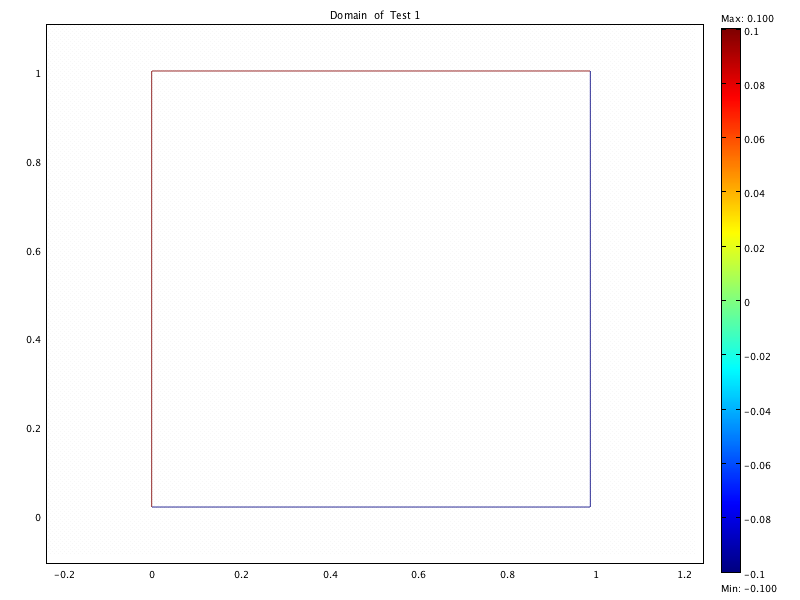
Fig. 1: Computational domain, boundary data, and mesh of Test 1

Figure 1 shows the computational domain, color plot of the force function $f_{1}+f_{2}$, and the mesh on which the numerical solution is computed. The mesh consists of $2360$ elements, and total number of degrees of freedom for the test is $12164$. $\Delta t=0.01$ is used in this test.

Figure 2 displays snapshots of the computed solution at three time incidences. Each graph contains color plot of the computed pressure $p_{h}^{n}:=\widetilde{p}_{h}^{n}+\alpha q_{h}^{n-1}$ and arrow plot of the computed displacement field $\mathbf{u}_{h}^{n}$. The three graphs on the first row are plotted on the computational domain $\Omega=(0,1)^{2}$, while three graphs on the second row are respectively deformed shape plots of the three graphs on the first row with $500$ times magnification, which shows the deformation of the square gel under the mechanical force $\mathbf{f}$ on the boundary. As expected, the gel is slightly rotated clockwise and is slightly bent near the top and bottom edges. We also note that the expected conserved quantities are indeed conserved in the computation, their respective values are given as follows:

$$C_{\mathbf{u}}=\int_{{\partial}\Omega}\mathbf{u}_{h}^{n}(x)\,dS\equiv 9.935\times 10^{-5},\quad C_{q}=\int_{\Omega}q_{h}^{n}(x)\,dx\equiv 9.935\times 10^{-5},$$

$$C_{\widetilde{p}}=\int_{\Omega}\widetilde{p}_{h}^{n}(x)\,dx\equiv 0,\quad C_{p}=\int_{\Omega}p_{h}^{n}(x)\,dx\equiv 1.489.$$

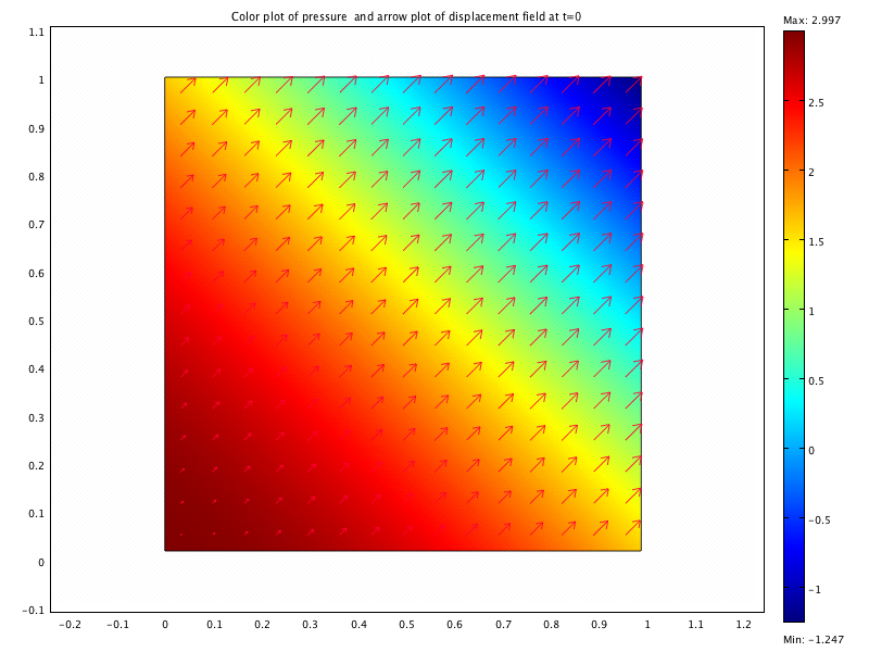
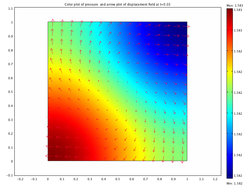
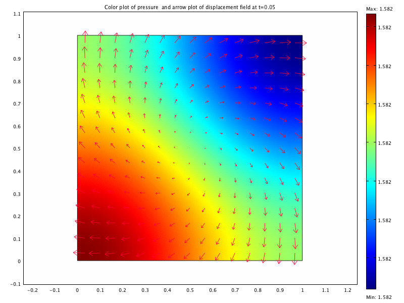
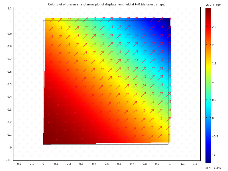
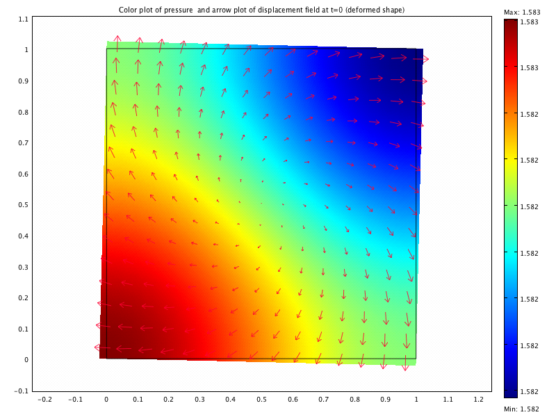
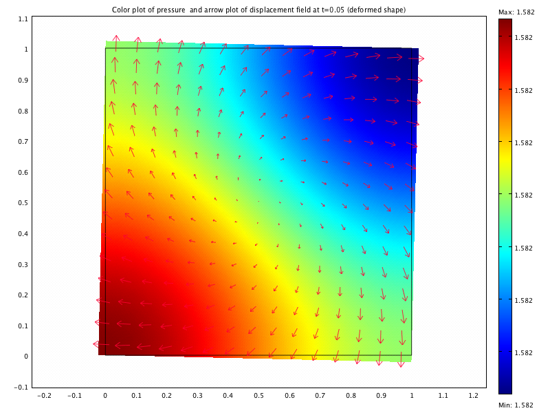
Fig. 2: Test 1: color plots of computed pressure $p_{h}^{n}$ and arrow plots of computed displacement $\mathbf{u}_{h}^{n}$ at $n=0,3,5$ (first row). Deformed shape plots of the graphs on the first row (second row). $\Delta t=0.01$.

Test 2: This test is same as Test 1 except $\mathbf{f}=(f_{1},f_{2})$ is changed to

$$f_{1}(x):=\left\{\begin{array}[]{rl}0.5&\qquad\mbox{for }x_{1}=0,\,0\leq x_{2}\leq 1,\\ -0.5&\qquad\mbox{for }x_{1}=1,\,0\leq x_{2}\leq 1,\\ 0&\qquad\mbox{for }x_{2}=0,1,\,0\leq x_{1}\leq 1,\end{array}\right.$$

$$f_{2}(x):\equiv 0.$$

So parallel forces of opposite directions are applied at the left and the right boundary of the square gel. Clearly, the compatibility condition (122) is satisfied.

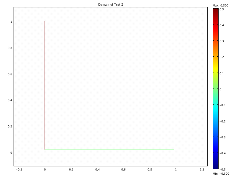
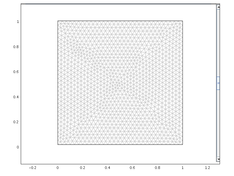
Fig. 3: Computational domain, boundary data, and mesh of Test 2

Like Figure 1, Figure 3 shows the computational domain, color plot of the force function $f_{1}+f_{2}$. The mesh parameters are also same as those of Test 1, including the time step $\Delta t=0.01$.

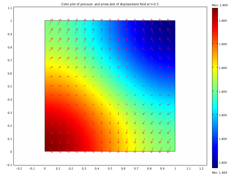
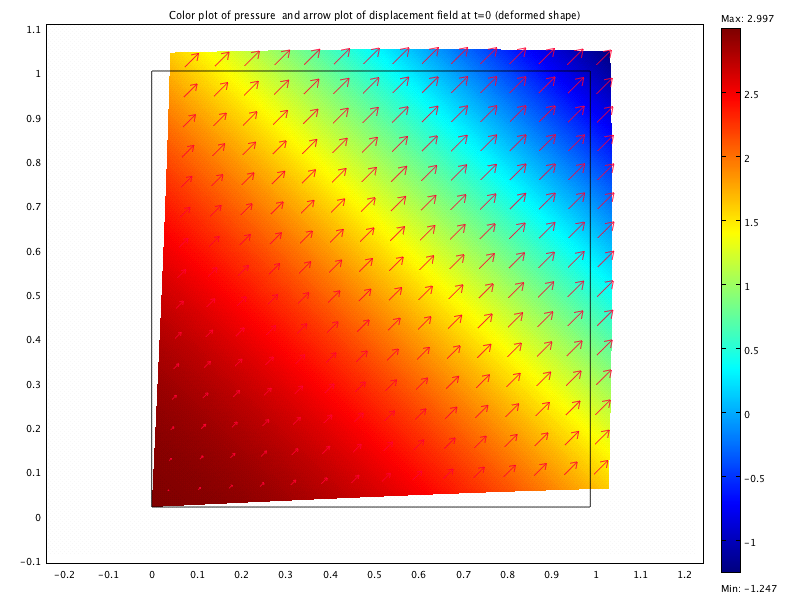
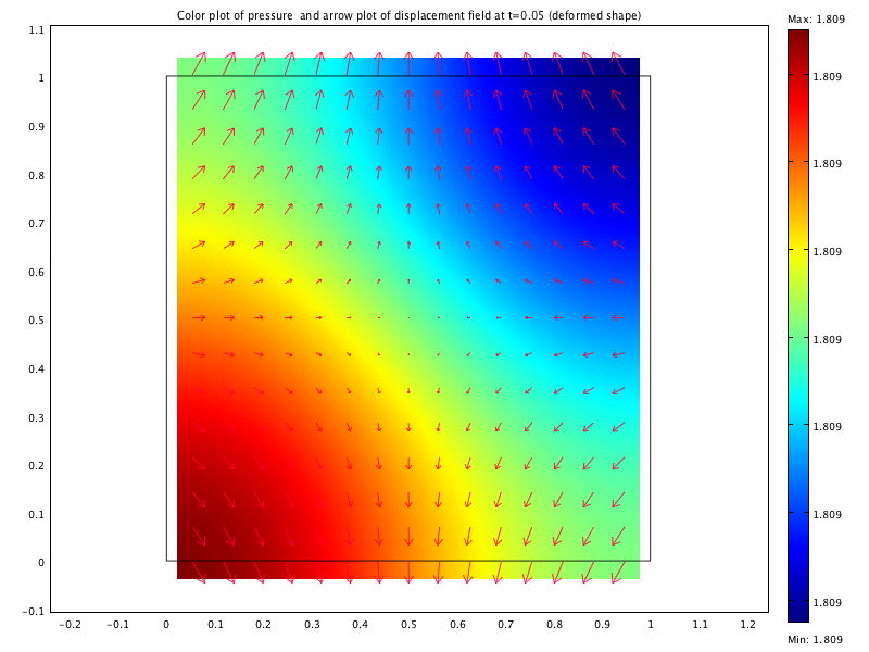
Fig. 4: Test 2: color plots of computed pressure $p_{h}^{n}$ and arrow plots of computed displacement $\mathbf{u}_{h}^{n}$ at $n=0,3,5$ (first row). Deformed shape plots of the graphs on the first row (second row). $\Delta t=0.01$.

Figure 4 is the counterpart of Figure 2 for Test 2. Since parallel forces of equal magnitude but opposite directions are applied on the left and the right boundary of the square gel, so the gel is squeezed horizontally. Because of the incompressibility of gel, the total volume must be conserved. As a result, the deformation in the vertical direction is expected. The second row of Figure 4 precisely shows such a deformation (with $500$ times magnification). It should be noted that the swelling dynamics of the gel goes super fast, it reaches the equilibrium in very short time. For the conserved quantities, $C_{q}$ and $C_{\mathbf{u}}$ are same as those in Test 1, and the other two numbers are given by

$$C_{\widetilde{p}}=\int_{\Omega}\widetilde{p}_{h}^{n}(x)\,dx\equiv 0.321,\qquad C_{p}=\int_{\Omega}p_{h}^{n}(x)\,dx\equiv 1.809.$$

Recall that $C_{\widetilde{p}}$ and $C_{p}$ depend on the force function $\mathbf{f}$.

Test 3: Same material parameters/constants and initial condition $\mathbf{u}_{0}$ as in Tests 1 and 2 are assumed. However, the computational domain is changed to the following one

$$\Omega:=\Bigl{\{}x\in\mathbf{R}^{2};\,\frac{x_{1}^{2}}{0.16}+\frac{x_{2}^{2}}{0.04}\leq 1\Bigr{\}},$$

and the external force function $\mathbf{f}$ is taken as

$$f_{1}(x):=\left\{\begin{array}[]{rl}0.5&\,\mbox{for }x\in{\partial}\Omega,\,-0.2<x_{1}<0,\\ -0.5&\,\mbox{for }x\in{\partial}\Omega,\,0<x_{1}<0.2,\end{array}\right.$$

$$f_{2}(x):\equiv 0$$

As in Test 2, the above $\mathbf{f}$ means that parallel forces of same magnitude but opposite directions are applied at the left half and the right half ellipse (boundary), however, these two forces now collide at two points $(0,\pm 0.2)$ on the boundary. Clearly, the compatibility condition (122) is satisfied.

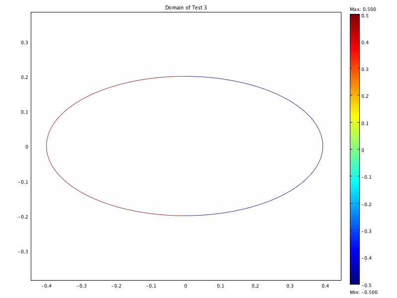
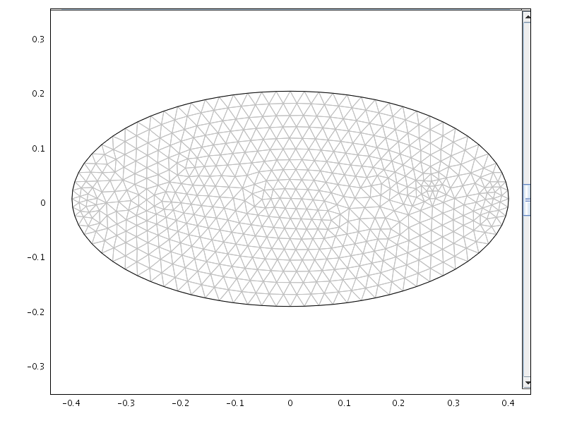
Fig. 5: Computational domain, boundary data, and mesh of Test 3

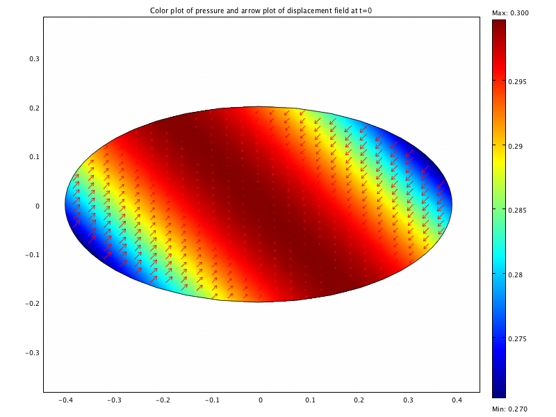
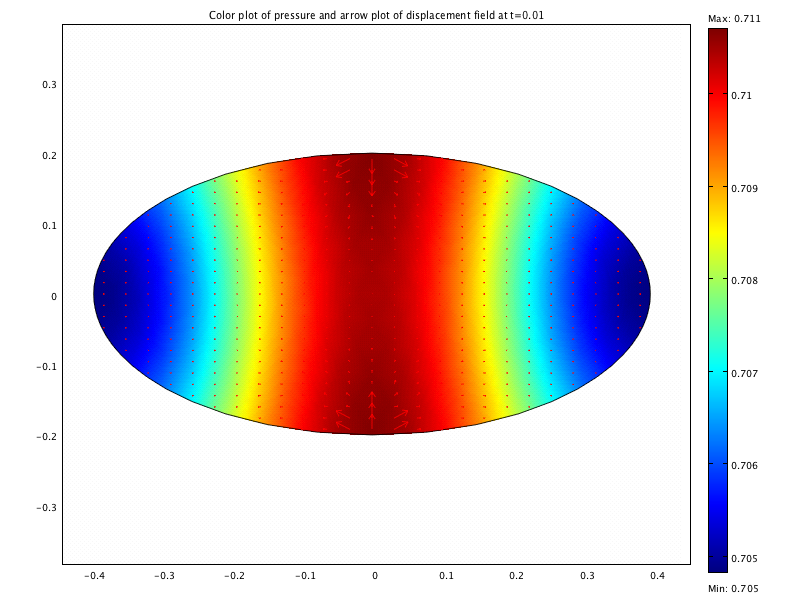
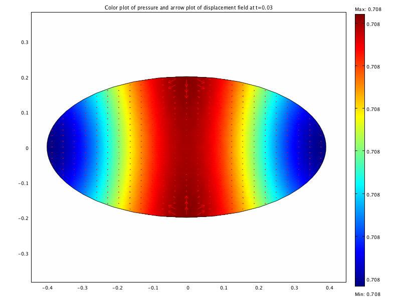
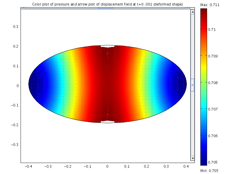
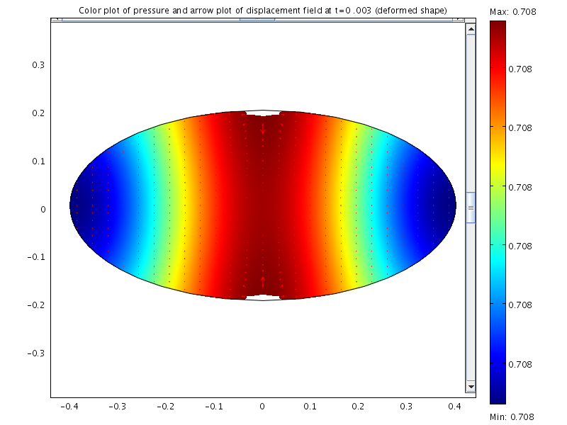
Fig. 6: Test 3: color plots of computed pressure $p_{h}^{n}$ and arrow plots of computed displacement $\mathbf{u}_{h}^{n}$ at $n=0,1,3$ (first row). Deformed shape plots of the graphs on the first row (second row). $\Delta t=0.001$.

Figure 5 is the counterpart of Figures 1 and 3 for Test 3. The mesh consists of $1200$ elements, and total number of degrees of freedom for the test is $6244$. A smaller time step $\Delta t=0.001$ is used in this test.

Figure 6 is the counterpart of Figures 2 and 4 for Test 3. The deformations displayed on the second row are magnified by $20$ times instead of $500$ times as in Figures 2 and 4. Due to curve boundary, the applied parallel forces of same magnitude but opposite directions collide at the boundary points $(0,\pm 0.2)$. It is expected that the gel should buckle around those two points, which is clearly seen in the plots on the second row of Figure 6. We also note that because relatively bigger forces are applied on the gel, the swelling dynamics of the gel goes even faster, hence, reaches the equilibrium quicker. This is the main reason to use a smaller time step for the simulation.

The conserved quantities for Test 3 are given as follows:

$$C_{\mathbf{u}}=\int_{{\partial}\Omega}\mathbf{u}_{h}^{n}(x)\,dS\equiv 4.902\times 10^{-6}, \qquad C_{q}=\int_{\Omega}q_{h}^{n}(x)\,dx\equiv 4.902\times 10^{-6},$$

$$C_{\widetilde{p}}=\int_{\Omega}\widetilde{p}_{h}^{n}(x)\,dx\equiv 0.105, \qquad C_{p}=\int_{\Omega}p_{h}^{n}(x)\,dx\equiv 0.178.$$

Acknowledgment: The first author would like to thank Professor Masao Doi of Tokyo University for introducing the gel swelling dynamic model to the author, and for his many stimulating discussions at IMA of University of Minnesota, where they both were long-term visitors in Fall 2004.

References

- [1] J. Bercovier and O. Pironneau, Error estimates for finite element solution of the Stokes problem in the primitive variables, Numer. Math., 33, pp. 211-224, (1979).
- [2] M. Biot, Theory of elasticity and consolidation for a porous anisotropic media, J. Appl. Phys. 26, pp. 182–185 (1955).
- [3] S. C. Brenner, A nonconforming mixed multigrid method for the pure displacement problem in planar linear elasticity, SIAM J. Numer. Anal., 30, pp. 116–135 (1993).
- [4] S. C. Brenner and L. R. Scott, The Mathematical Theory of Finite Element Methods, third edition, Springer, 2008.
- [5] F. Brezzi and M. Fortin, Mixed and Hybrid Finite Element Methods, Springer, New York (1992).
- [6] P.G. Ciarlet, The Finite Element Method for Elliptic Problems, North-Holland, Amsterdam (1978).
- [7] O. Coussy, Poromechanics, Wiley & Sons, 2004.
- [8] M. Doi, private communication.
- [9] M. Doi, Dynamics and Patterns in Complex Fluids, A. Onuki and K. Kawasaki (eds.), p. 100, Springer, New York (1990).
- [10] M. Doi and S. F. Edwards, The Theory of Polymer Dynamics, Clarendon Press, Oxford (1986).
- [11] D. Gilbarg, N.S. Trudinger, Elliptic Partial Differential Equations of Second Order, Second Edition, Springer, New York, 2000.
- [12] V. Girault and P.A. Raviart, Finite Element Method for Navier-Stokes Equations: theory and algorithms, Springer-Verlag, Berlin, Heidelberg, New York (1981).
- [13] I. Hamley, Introduction to Soft Matter, John Wiley & Sons, 2007.
- [14] M. A. Murad and A. F. D. Loula, Improved accuracy in finite element analysis of Boit’s consolidation problem, Comput. Methods in Appl. Mech. and Engr, 95, pp. 359–382 (1992).
- [15] J.E. Roberts and J.M. Thomas, Mixed and hybrid methods, in Handbook of Numerical Analysis, Vol. II, North-Holland, New York,, pp. 523–639 (1991).
- [16] T. Takigawa, T. Ikeda, Y. Takakura, and T. Masuda, Swelling and stress-relaxation of poly(N-isopropylacrylamide) gels in the collapsed state, J. Chem. Phys., 117, pp. 7306-7312 (2002).
- [17] T. Tanaka and D. J. Fillmore, Kinetics of swelling of gels, J. Chem. Phys. 70, 1214 (1979).
- [18] R. Temam, Navier-Stokes Equations, Studies in Mathematics and its Applications, Vol. 2, North-Holland (1977).
- [19] T. Yamaue and M. Doi, Theory of one-dimensional swelling dynamics of polymer gels under mechanical constraint, Phys. Rev. E 69, 041402 (2004).
- [20] T. Yamaue and M. Doi, Swelling dynamics of constrained thin-plate under an external force, Phys. Rev. E 70, 011401 (2004).