A simple model for the relationship between star formation and surface density

Abstract

We investigate the relationship between the star formation rate per unit area and the surface density of the ISM (the local Kennicutt-Schmitt law) using a simplified model of the ISM and a simple estimate of the star formation rate based on the mass of gas in bound clumps, the local dynamical timescales of the clumps, and an efficiency parameter of around $\epsilon\approx 5$ per cent. Despite the simplicity of the approach, we are able to reproduce the observed linear relation between star formation rate and surface density of dense (molecular) gas. We use a simple model for the dependence of H₂ fraction on total surface density to argue why neither total surface density nor the Hi surface density are good local indicators of star formation rate. We also investigate the dependence of the star formation rate on the depth of the spiral potential. Our model indicates that the mean star formation rate does not depend significantly on the strength of the spiral potential, but that a stronger spiral potential, for a given mean surface density, does result in more of the star formation occurring close to the spiral arms. This agrees with the observation that grand design galaxies do not appear to show a larger degree of star formation compared to their flocculent counterparts.

1 Introduction

1.1 Observational Background

The dependence of the star formation rate per unit area on the surface density of the ISM in a galaxy is one of the most highly speculated problems in extra-galactic surveys, as well as theoretical analysis of star formation. The star formation law predicts both the amount of star formation and the degree of stellar feedback in a galaxy, and is consequently a vital requirement for models of galaxy evolution (e.g. Tan, Silk & Balland 1999; van den Bosch 2000; Springel 2000; Hou, Prantzos & Boissier 2000; Springel & Hernquist 2003).

Schmidt (1959) related the star formation rate per unit volume, $\rho_{\rm SFR}$, to the gas density, $\rho$, in a galaxy according to $\rho_{\rm SFR}\propto\rho^{m}$. An observational law for star formation rate per unit surface area, $\Sigma_{\rm SFR}$ in terms of the mean gas galactic surface density, $\Sigma$, viz. $\Sigma_{\rm SFR}\propto\Sigma^{n}$ was established by Kennicutt (1989), and since then numerous surveys have attempted to find a universal value of $n$. Kennicutt (1989, 1998) investigated a global star formation law in star-forming galaxies and found $n=1.3\pm 0.3$ from a sample of 97 galaxies including normal spirals and starbursts, for gas surface densities of a few M_⊙ pc^-2 to around $10^{4}$ M_⊙ pc^-2, although it should be noted that at a given $\Sigma$, the scatter in $\log\Sigma_{\rm SFR}$ is generally more than $\pm 0.5$. Other surveys include Gao & Solomon (2004b), who trace both the densest gas, using HCN, and the total gas in a galaxy. They obtain different relations depending on what is meant by $\Sigma$. For $\Sigma$ measuring dense gas they find $n$=1 whereas for $\Sigma$ measuring total gas density they find $1.73$.

The local relationship between star formation rate per unit area and surface density (what we call here the local Kennicutt-Schmidt law), has also been examined for individual galaxies. Wong & Blitz (2002) used radially averaged values of the star formation rate and surface densities for 6 galaxies, finding n=1.2–2.1. Kennicutt et. al. 2007 also obtained $n=1.56\pm 0.04$ for M51, by sampling the H_α emission and total surface density over 500 pc size regions (see also Schuster et al. 2007). There is a slightly less steep correlation ($n=1.37\pm 0.03)$ for the surface density of molecular gas, but no correlation with the HI gas. Similarly Heyer et al. (2004) found $n=1.36$ for M33, when considering the molecular gas alone, but a much steeper dependence ($n=3.3\pm 0.1$) on the total gas surface density.

In fact the general consensus from these results is that a well-defined local star formation law holds only for the molecular gas in these galaxies. This conclusion is further endorsed by recent results from the THINGS survey (Bigiel et al., 2008), which show that there is no correlation between the Hi and the star formation rate – $\Sigma_{\rm SFR}$ is multivalued for a given density of Hi. Their results also indicate a fairly sharp transition from a regime where gas is predominantly Hi, to where gas is mainly molecular. Thus in the Hi regime, $\Sigma_{\rm SFR}$ varies very steeply with $\Sigma$, whereas in the H₂ regime, $n$ is roughly 1. For the total gas surface density, $n$ lies between 1 and 3, although it is evident that the data does not give a good linear fit.

1.2 Theoretical interpretations

Several theoretical explanations of the Kennicutt-Schmidt law have also been advanced. All interpret $\Sigma$ as being the total surface gas density. Since star formation occurs in a chaotic or turbulent environment, a natural explanation is that turbulence somehow regulates how much gas exceeds the high densities required for star formation. Elmegreen (2002) and Krumholz & McKee (2005) assume a probability density function of densities in a turbulent regime to obtain a star formation law with $n=1.4$. For Elmegreen (2002), this involves assuming an unknown star formation efficiency ($\epsilon$), but Krumholz & McKee (2005) instead determine the star formation rate efficiency, thus eliminating $\epsilon$. This is essentially the derived star formation rate divided by the total possible star formation rate if all gas at a particular density was turned into stars.

Krumholz & Tan (2007) and Krumholz & Thompson (2007) further compare the turbulence regulating model of star formation with observations. Krumholz & McKee (2005) predict that the star formation rate efficiency is $\sim 0.013$, independent of density. Their observed estimates of the star formation rate efficiency (Krumholz & Tan, 2007) are consistent with this prediction. However the uncertainties (in particular for lifetimes for a given tracer) do not rule out a star formation rate efficiency which increases with density either. Krumholz & Thompson (2007) also determine CO and HCN luminosities, and show that the star formation rate is linear with relation to L(HCN) and nonlinear for L(CO).

An alternative possibility is to estimate the star formation rate from cloud-cloud collisions. In this case $\Sigma_{\rm SFR}$ is proportional to the surface density over the collision time, which in turn is dependent on the shear in the disc, measured by the orbital angular velocity $\Omega$. This yields an alternative form of the Schmidt law, $\Sigma_{\rm SFR}\propto\epsilon\Omega\Sigma^{N}$ where $\epsilon$ is the star formation efficiency and $N=1$ (Wyse, 1986; Wyse & Silk, 1989; Tan, 2000). Silk (1997) explicitly includes the star formation efficiency by assuming that star formation is self regulating in the disc, obtaining $\Sigma_{SFR}\propto\Sigma^{1.78}$.

In addition to the observational surveys, several numerical simulations have investigated star formation rates in galaxy simulations (Li et al., 2006; Robertson & Kravtsov, 2008; Tasker & Bryan, 2008). However a major problem with numerical evaluations of the star formation rate is that it is dependent on what assumptions are made about the conditions for forming sink particles at high densities, or for taking account of possible forms of stellar feedback. A density threshold is required, as well as a star formation efficiency, and so the degree of star formation in these simulations is also dependent on both these parameters. Saitoh et al. (2008) performed simulations with varying thresholds and star formation efficiencies, concluding that the star formation rates and Kennicutt-Schmidt law do not significantly change provided there is a high threshold density. However an estimation of the star formation rates from first principles, without these approximations, is beyond current capabilities.

Tasker & Tan (2008) perform similar models to those of the current paper, and likewise do not include any star formation prescription. In their simulations there is no underlying spiral potential, rather numerous flocculent spiral arms cover the disc. In agreement with Dobbs (2008) they find that GMCs form by agglomeration via collisions, although collisions occur throughout the disc whereas in Dobbs (2008), collisions between clouds are largely confined to the spiral arms. They do not make any estimates of the star formation rate from their results, however they do show that the number of collisions between clouds is consistent with the model presented in Tan (2000).

1.3 The current paper

One approach to trying to understand the physics underlying the basis of the Schmitt-Kennicutt relations is to undertake ever more detailed numerical simulations with ever increasing quantities of input physics (e.g. Susa 2008; Shetty & Ostriker 2008; Agertz et al. 2009). In this paper, we take an alternative approach and ask the question: how little input physics, and how few assumptions do we have to make, in order to obtain relations which resemble the observational findings to a reasonable degree? In this manner we hope to be able to obtain some understanding of what the fundamental drivers for such a relationship might be.

The calculations presented in this paper make use of the simplified numerical simulations which have already been published in Dobbs (2008). The simulations were performed using Smoothed Particle Hydrodynamics, and include magnetic fields and self-gravity. We do not include the star formation process itself nor any subsequent stellar feedback. Thus the gas is supported against collapse by thermal and magnetic pressure in the lower surface density calculations. In the higher surface density results, we run the calculations until collapse occurs. The difficulty with the assumed lack of feedback is that we are restricted to relatively low surface density calculations. The calculations which have been selected for analysis in this paper are shown in Table 1. These calculations, with the exception of model C, are described in Dobbs (2008), but we also provide details below.

1.3.1 Details of numerical models

The calculations model a 3D gaseous disc between radii of 5 and 10 kpc. The gas is assumed to orbit in a fixed galactic gravitational potential. The potential includes a halo (Caldwell & Ostriker, 1981), disc (Binney & Tremaine, 1987) and 4 armed spiral component (Cox & Gómez, 2002). The gas is initially assigned velocities according to a flat rotation curve determined by the disc potential, and in addition a velocity of dispersion of 6 km s^-1 is superposed.

Models A-D have identical potentials but vary in their mean gas surface densities and therefore compare surface density. The total mass of the disc is $1\times 10^{9}$ M_⊙ in the 4 M_⊙ pc^-2 model, and 5$\times 10^{9}$ M_⊙ in the 20 M_⊙ pc^-2 model. The simulations all use 4 million particles, hence the highest mass resolution is 250 M_⊙, and the lowest 1250 M_⊙. Models A, E, F and G have the same mean gas surface densities but adopt different strength for the spiral potential.

In keeping with our aim for minimal input physics, the simulations are very simplistic. In particular, all the calculations in Table 1 assume an interstellar medium which has two isothermal components, one cool and one warm. We omit thermal considerations and so there is no transition between the two phases; the cool gas remains cool and the warm gas remains warm, throughout. We use the same thermal distribution in all the calculations and only vary the global surface density and/or the shock strength. The cool gas is taken to have a temperature of $T=100$ K, and we will think of it as representing molecular gas (H₂). The warm gas is taken to have $T=10^{4}$ K, and we will think of it representing atomic gas (Hi). In all cases the cool and warm gas comprise equal mass in the simulations. It is of course possible to include thermal effects such as heating and cooling – see, for example (Dobbs et al., 2008) (although these did not include self-gravity) but that is not the purpose of the current exercise.

The initial scale heights of the warm and cold warm components are 150 and 400 pc respectively, giving a mean smoothing length of 40 pc. However with time the scale heights decrease to 20-100 pc and 300 pc.

These calculations do not include sink particles, although the gas is self-gravitating. In the lower surface density results ($\Sigma\leq 10$ M_⊙ṗc^-2), the cool gas is sufficiently supported by magnetic and thermal pressure, and the (typically supersonic) velocity dispersion of the gas. However in the higher surface density results, runaway gravitational collapse does occur. The calculations were run for either 250 Myr, or until the calculation is halted by collapse. The maximum timestep in the calculations (and frequency of dumps) is 2 Myr, but individual particles timesteps can be much less (Bate, 1995).

Model	$\Sigma$ (M⊙ pc-2)	F (%)	Qc	Qh
A	4	4	0.5	5
B	8	4	0.25	2.5
C	16	4	0.25	2.5
D	20	4	0.1	1
E	4	2	0.5	5
F	4	8	0.5	5
G	4	16	0.5	5

Table 1: The calculations from Dobbs (2008) which are used in this paper. All the calculations use 4 million particles and are isothermal. In these calculations, half the gas cold (100 K) and half warm ($10^{4}$ K), and the ratio of thermal to magnetic energy ($\beta$) is 0.4 in the cold gas. $F$ is a measure of the strength of the potential, and $Q$ is the Toomre parameter ($Q_{c}$ for the cool gas and $Q_{h}$ for the warm gas). The determination of all these quantities is described in Dobbs (2008). Models A-D compare surface density, and E-G shock strength.

2 Estimating $\Sigma_{\rm SFR}$ in the numerical simulations

In this paper we shall assume that star formation occurs only in those regions of the ISM which are bound, and at a rate determined simply by the local dynamical timescale.

2.1 Gravitationally bound gas

We must first find a means of identifying which regions of the ISM are gravitationally bound at a particular moment. It needs to be borne in mind that while unbound gas can obviously become bound, it is also possible for bound gas to become unbound, despite the lack of feedback. This can come about for example as the gas accelerates out of a spiral arm, flowing over the ridge of the spiral potential, becoming sheared and longitudinally stretched as it does so.

We determine the mass of bound gas using the output from a simulation at a given time frame (after 250 Myr except for models C and D, where the times are 200 Myr and 140 Myr). The particular timeframe selected is not important, provided the time is not too near the beginning of the simulation, where the amount of bound gas will be underestimated.

In order to determine the mass of bound gas, we first sort the particles according to density. We select the most dense particle, and all particles within a radius of a smoothing length of that particle. Then we determine the gravitational, kinetic, thermal and magnetic energies for this group of particles. If $(E_{k}+2E_{th}+E_{mag})/E_{grav}<1$, the gas is assumed to be bound and the radius increased until the gas becomes unbound. Then the particles which are bound are recorded and their mass added to the total mass of bound gas. If on the other hand the gas is unbound, the gas particles are discarded from the list. We also performed this analysis using solely either just the kinetic energy or both the kinetic and thermal energy.

Using this method, the bound gas is situated in discrete clumps (which are spherical by assumption). Fig 1 shows the location of bound gas for a small section of the disc, for the simulation Model B with $\Sigma=8$ M_⊙ pc^-2. The colours indicate whether just the kinetic, the kinetic and thermal, or the kinetic, thermal and magnetic energies are included. As expected, when all three energies are included, the extent of a clump which is bound becomes smaller, whereas the clumps are more extended (particularly true in the higher surface density calculations) when only the kinetic energy is considered. In other simulations which investigate the Kennicutt-Schmidt law, magnetic fields are not included (Bottema, 2003; Tasker & Bryan, 2006; Li, Mac Low & Klessen, 2006; Booth, Theuns & Okamoto, 2007), so by default only the kinetic and thermal energies can be used.

In Fig. 1 the bound gas is dominated by two massive clumps which are just leaving the arms. These are more extended since they have higher densities and lower velocity dispersions than clumps in the spiral arms. The gravitational energy of these clumps is also high since they are centrally condensed. Essentially these might be taken to represent massive Giant Molecular Clouds (GMCs), which formed in the spiral arms and are now entering the interarm regions, leaving only less massive clumps in the spiral arms. We also see that there are numerous bound clumps in the interarm regions. Overall in the bound gas there is no particular evidence of spiral structure other than the two massive ‘GMCs’. The degree of bound gas in the interarm regions reflects the fact that the velocity dispersions of clumps in the interarm regions are lower than in the spiral arms. In the interarm regions there are fewer collisions and fewer interactions between clumps.

From hereon, we shall generally assume that the calculation of bound gas includes the thermal and magnetic energy, as well as the kinetic. This assumption minimises the amount of ’bound’ gas present in the simulations. Using the kinetic energy alone tends to produce an unrealistically high fraction of bound gas. In Fig. 2 we plot the cumulative surface density of bound gas versus number density for model B. Here the cumulative mean surface density of bound gas is defined as $\Sigma_{\rm bound}(n)=M_{\rm bound}(n)/A$, where $M_{\rm bound}(n)$ is the mass of bound gas in clumps with maximum density $>n$, and $A$ is the area of the galactic disc. It can be seen that the maximum density in a clump typically must be $n>10^{4}$ cm^-3 to obtain bound regions. This condition is less stringent if thermal and/or magnetic energies are ignored. Fig. 2 also shows that the bound gas represents 6 % of all the gas in the disc.

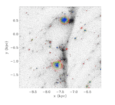
Figure 1: The location of bound gas is shown for a small section of the disc from the $\Sigma=8$ M_⊙ pc^-2 simulation Model B. Blue indicates regions which are bound when the kinetic, thermal and magnetic energies are included, green, the kinetic and thermal, and red, just kinetic. If only the kinetic energy is used to determine whether regions are bound, the clumps are clearly more extended. Two large and massive complexes are moving away from the spiral arms, which have high density and low velocity dispersions, so are strongly bound. There is also a considerable number of bound clumps in the interarm regions.

Figure 2: The mass of bound gas is plotted versus number density $n$ when $\Sigma=8$ M_⊙ pc^-2 (Model B). Particles are sorted by density, and so $n$ represents the maximum density in a given bound region. The mass indicated on the $y$-axis is cumulative, and thus represents the total mass of bound gas in regions with a maximum density $>n$. The mass of bound gas is calculated using the kinetic, thermal and magnetic energy. Clumps with densities $<10^{4}$ cm^-3 do not tend to contain bound gas. The right hand $y$-axis indicates the percentage of the total gas in the disc which is bound.

2.2 Star formation rate

In order to determine the star formation rate, having determined an estimate of the amount of bound gas, we require an estimate of the local timescale for star formation. As we mentioned above we take this to be the local dynamical timescale of the gas,

$$t_{\rm dyn}=\sqrt{\frac{3\pi}{16G\langle\rho\rangle}}\,.$$ (1)

Here $\langle\rho\rangle$ is the median density of a clump. An alternative would be to use the volume average density, $\bar{\rho}$, but we find that this does not lead to a noticeable difference in the results. The star formation rate of a particular clump is then assumed to be $\dot{M}=M_{\rm bound}/t_{\rm dyn}$ where $M_{\rm bound}$ is the mass of bound gas in a clump and $t_{\rm dyn}$ the dynamical timescale of that clump given by equation 1. The star formation rate per unit area, averaged over a given region, is then

$$\Sigma_{\rm SFR}=\frac{\sum_{i=1}^{N}\dot{M_{i}}}{A}$$ (2)

where the summation is over all ($N$) bound clumps, and $A$ is the area of the region under consideration.

It is well known that star formation is a relatively inefficient process in that not all the bound gas is converted to stars on a local dynamical timescale. We can allow for this by including an efficiency parameter $\epsilon$. In this case the star formation rate would be

$$\Sigma_{\rm SFR}=\frac{\sum_{i=1}^{N}\epsilon\,\dot{M_{i}}}{A}$$ (3)

where $\epsilon$ is the constant star formation efficiency. However we do not consider the evolution of the gas once it becomes bound. Rather than assume a value of $\epsilon$ for the star formation rate, we consider what value of $\epsilon$ would be required to fit observations. As we expect the value of $\epsilon$ turns out to be small, justifying a posteriori our decision not to remove mass from the ISM in order to model star formation.

3 Results

We now apply these simple assumptions to the numerical simulations.

3.1 Global star formation rate versus mean surface density

In Fig. 3, we plot the star formation rate per unit area averaged over for the whole disc in Models A-D, estimated by using Eqn 2. This is then the equivalent of the global Kennicutt-Schmidt law. Points are shown at three different time frames for each surface density to illustrate the point that the ISM is not evolving significantly through the simulations. The points do show a correlation of star formation rate with surface density, roughly of the form $\Sigma_{\rm SFR}\propto\Sigma^{2.8}$. However, even though the range in surface densities is not large, the figure does indicate that the relation we find is not a simple power law, with the dependence becoming shallower at higher densities, or equivalently showing a sharp downturn at low surface densities.

The estimated star formation rates in our models are much higher than observed since the formula in equation 2 assumes a star formation efficiency of 100%. We can however estimate what efficiency would correspond to observations. Comparing the star formation rate at a surface density of 10 M_⊙ pc^-2 to Fig. 2 of Kennicutt (1998), we find that we need to assume an efficiency of 5% ($\epsilon=0.05$) in order to produce star formation rates compatible with observations.

We can also consider the star formation rate efficiency by calculating the ratio of $\Sigma_{\rm bound}/\Sigma_{\rm total}$, as shown on Fig. 2. This fraction is 1.5 %, 6 %, 5 % and 6 % with surface densities of 4, 8, 16 and 20 M_⊙ pc^-2. Thus the proportion of gas undergoing star formation is similar in the regime where the slope of $\Sigma_{\rm sfr}$ starts to depend linearly with $\Sigma$, but somewhat lower at the lowest surface density.

3.2 Local star formation rate versus local surface density

With effectively only 4 data points, evaluating the dependence of the star formation rate per unit area on surface densities averaged over the entire disc is limited. We have therefore divided each galaxy into 500 x 500 pc squares (the resolution of the recent THINGS results). We then calculate the star formation rate per unit area from the surface density of bound gas in each square, also assuming a star formation efficiency of $\epsilon=0.05$, in order to compare with observations. In Fig. 4, we have combined the star formation rates from a quarter of the disc in the calculations of Models A, B and D, which have mean surface densities of 4, 8, and 20 M_⊙ pc^-2 into a single plot, thus acquiring more data points and a greater range of densities. In the figure we plot for each square the estimated star formation rate per unit area versus the mean ISM surface density (cool and warm gas).

In Fig. 4 we have overplotted our star formation rates on Fig. 8 of Bigiel et al. (2008), which shows the star formation rate over the spirals in their sample versus surface density, as well as the globally averaged star formation rate for the galaxies in the survey by Kennicutt (1998). Our simplified model seems to fit the observational data reasonably well. Our distribution appears to support the decline in the star formation rate below around $\Sigma=10$ M_⊙ pc^-2, as seen in Bigiel et al. (2008). Our points also agree with the lower end of those from Kennicutt (1998), similarly indicating a possible relative decline in star formation at low densities. In fact the star formation rate appears to show a change in slope, and there is much more scatter at surface densities less than 10 M_⊙ pc^-2. To clarify this we have binned the points from our results in Figure 5. There we show the mean star formation rate at each surface density, together with scatter indicated as error bars at one standard deviation. There is evidently more scatter at low densities and a steeper slope. We discuss this more in the next sections.

Fig. 5 also shows the difference when we take only the regions with bound gas (blue points), and when all 500 $\times$ 500 pc regions covering the disc are considered, even if they contain no bound gas (red points). For the latter we assume a maximum star formation rate of $10^{-6}$  M_⊙ kpc^-2 yr^-1 in the squares where there is no bound gas, rather than zero, in order to calculate the error bars. This estimate is approximately the lowest resolvable star formation rate in our simulations. As expected the slope is steeper when regions with this minimal star formation rate are included (red points). Also the figure indicates that regions which do not contain bound gas tend to have average surface densities of less than $\sim 10$ M_⊙ pc^-2.

Figure 3: The estimated global star formation rate ($\Sigma_{\rm bound}/t_{\rm dyn}$) is shown versus mean surface density for the galaxies in Models A, B, C and D. The star formation rate does not show a good linear fit with surface density, and at low densities at least, is steeper than the observed Kennicutt-Schmidt law.

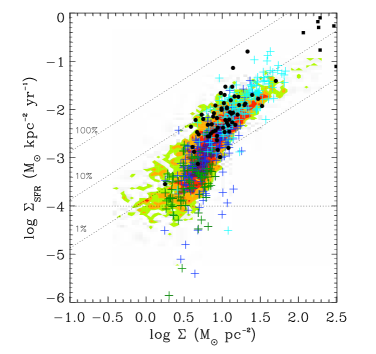
Figure 4: The star formation rate is plotted for the 4 (dark green crosses, Model A), 8 (blue crosses, Model B) and 20 M_⊙ pc^-2 (cyan crosses, Model D) models, assuming a star formation efficiency of $\epsilon=0.05$. The black circles are normal spirals, and the black squares starburst galaxies from the survey of Kennicutt (1989). These are all overplotted on Fig. 8 (middle right panel) of Bigiel et al. (2008), which is the green and orange contour plot visible in the background. This shows the star formation rate versus surface density of Hi and H₂ sampled over 500 pc² regions from 7 spiral galaxies. The green, orange, red and magenta contours indicate 1, 2, 5 and 10 data points respectively. The star formation rates from the simulations and the observed data agree reasonably, and both show a downturn in slope at around $\Sigma=10$ M_⊙ pc^-2.

3.3 The local Kennicutt-Schmidt law for different tracers

It has become apparent from recent observations that the star formation law varies for different tracers. The star formation law is shallower for high density gas, e.g. H₂, HCN (Gao & Solomon, 2004b; Bigiel et al., 2008), so $\Sigma_{\rm SFR}$ goes roughly as $\Sigma(H_{2})^{1.0}$. By comparison the star formation rate varies as approximately $\Sigma^{1.5}$ when $\Sigma$ is the surface density of all gas, i.e. Hi and H₂. The law becomes even steeper when just Hi is considered (Heyer et al., 2004; Kennicutt & et. al., 2007; Bigiel et al., 2008), suggesting that Hi is not a good measure of local star formation. Krumholz & Thompson (2007) propose that the transition from superlinear to linear occurs when the density at which a molecule is excited is similar to the median density of the galaxy.

A common feature in the results from the simulations and the results of Bigiel et al. (2008) is that there is much more scatter at low surface densities compared to high. A likely explanation is that at low densities the gas can exhibit a range of distributions – the gas can lie in a few dense bound clumps undergoing star formation, or alternatively in a more diffuse medium with very little star formation. At higher densities, much more of the gas in a given region is likely to be in bound clumps undergoing star formation and the possibility of larger volumes of diffuse gas is diminished. Bigiel et al. (2008) express this as the filling factor of the gas, i.e. the ratio of gas as high densities where stars are forming. The high density tracers preferentially select the top (highest star formation rate) points from the distribution for all the gas.

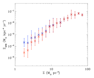
Figure 5: The star formation rate for points in the simulations with 4, 8 and 20 M_⊙ pc^-2 (as shown in Fig. 4) is binned according to surface density. The scatter in the average star formation rate is then shown as 1-$\sigma$ error bars. The different points indicate whether regions without bound gas are included. The blue data points exclude regions in which none of the gas is bound. The red data points are inclusive of those regions which contain no bound gas (and are therefore not seen on Fig. 4), where instead we assume a maximum star formation rate of $10^{-6}$ M_⊙ kpc^-2 yr^-1.

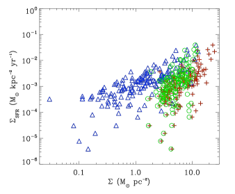
Figure 6: The star formation rate is plotted against surface density for 500 pc² regions from Model B, where the mean surface density is 8 M_⊙ pc^-2. The red crosses represent points where no density cut is imposed. The blue triangles correspond to points which only include gas of density above 10^-23 g cm^-3. The slope is clearly shallower when only the denser material is used. Finally we selected gas with densities $<10^{-23}$ g cm^-3 (green circles), for which the slope becomes steeper.

We can test directly the likely effect of using different tracers in the simulations. As we have mentioned above the cool component of our model ISM can be seen as a proxy for molecular gas, whereas the warm component can be seen as a proxy for atomic gas. It is the cool gas which is more severely affected by the spiral structure, and therefore the cool gas which is more likely to be contained in bound entities. The warm gas, with sound speeds comparable to the potential depths of the spiral potential, tends to be less affected by the spiral arms and less easily assimilated into bound clumps. Thus, although the evolution of different chemical species is not followed in these simulations, we can use a density cut to select particles over a given density. In the observations, it is not whether or not the gas is molecular that defines the slope of the power law, it is merely that the molecular gas traces the denser parts of the ISM.

Fig. 6 shows the star formation rate per unit area against surface density for Model B when the surface density of all the gas is used, compared to when there is a density cut of 10^-23 g cm^-3. With the density cut, the surface densities are only calculated using the gas with density above this threshold, whilst the star formation rate is the same, thus points are shifted to the left in the Figure. At low surface densities, much less of the gas is at high densities, so the points are shifted much further. Hence the slope is shallower compared to the relation for all the gas and indeed tends towards the observed linear relation between star formation rate and surface density for the densest gas. We also selected gas below this threshold, and as expected a steeper relation ensues. Gnedin et al. (2008) obtain similar results by plotting the star formation rate against densities of Hi, H₂ and Hi+H₂ calculated in their simulations.

In our models the slope of $\Sigma_{\rm SFR}$ changes continuously from a very steep slope at low density criterion to linear with a higher density criteria. The roughly linear relation to surface density for gas above 10^-23 g cm^-3 suggests gas above this density is involved in star formation. Actually, only about a quarter of this gas is gravitationally bound. We therefore also calculated $\Sigma_{\rm SFR}$ with a cut of 10^-22 g cm^-3, in which case nearly all the gas is bound. The slope is approximately 1.0 in both cases, but the points are shifted to lower surface densities with the higher surface density cut.

3.4 Theoretical interpretation

There seems to be evidence from the observations, that for molecular tracers which presumably correspond to the higher density gas, $\Sigma_{\rm SFR}\propto\Sigma^{n}$ with $n=1$. This relation can be reproduced in our simulations by considering only the highest density gas. This relation also holds at the higher surface densities even when $\Sigma$ is the total surface density. This appears to be approximately when $\Sigma>10$ M_⊙ pc^-2, where most of the gas is cool/molecular (Dobbs et al., 2008; Krumholz et al., 2008).

This raises two questions: why is the relationship linear, and why is it much steeper than linear at lower surface densities?

3.4.1 A shallower local Kennicutt-Schmidt relation?

At high surface densities a shallower relation of the form $\Sigma_{\rm SFR}\propto\Sigma^{1.0}$ is found. This contradicts the straightforward expectation of most theoretical models (see Section 1.2, and, for example, the discussion in Section 5 of Kennicutt, 1998), in which the star formation rate is presumed to depend on the local surface density divided by an appropriate timescale. For example one might take $\Sigma_{\rm SFR}\propto\Sigma/t_{\rm dyn}$. Then assuming that $t_{\rm dyn}\propto\Sigma^{-0.5}$, one finds that $\Sigma_{\rm SFR}\propto\Sigma^{1.5}$, in rough agreement with the Kennicutt-Schmidt law.

One possible explanation for this discrepancy, as also suggested by Krumholz & Thompson (2007), might be that star formation only takes place in the densest gas, regardless of the average surface density. Thus for determining the star formation rate, $\rho$ is effectively constant, and therefore the local dynamical time given by a formula such as Equation 1 is also roughly constant.

To examine this further, we plot in Figure 7 the various dynamical times of the various bound clumps against the mean local surface density of the 500 $\times$ 500 pc² areas in which they are found in Model B, the 8 M_⊙ pc^-2 simulation. As can be seen from the figure, the dynamical time shows no particular correlation with surface density. Thus to a first approximation, the local star formation rate per unit area just depends in a linear fashion on the local mean surface density of bound gas. The exception in our calculations is the lowest surface density case (model A) where there is a large increase in the dynamical time at low surface densities.

Our hypothesis differs mainly from Krumholz & Thompson (2007) in that we do not suppose a $\Sigma^{1.5}$ relation for the total gas. Instead, as expressed in Section 3.3, we expect a large degree of scatter between the star formation rate and $\Sigma$ at low surface densities, depending on the local environment of the gas, whilst a linear relation prevails at high surface densities.

3.4.2 $\Sigma$(total) versus $\Sigma$(H₂)

The difference between the tracers can be illustrated in the following manner. Supposing that the fraction of the ISM which is in molecular form, $f(H_{2})$, is a monotonically increasing function of the local surface density $\Sigma$. As an example we take

$$f(H_{2})=\left(\frac{\Sigma}{\Sigma_{0}}\right)^{\alpha},$$ (4)

for $\Sigma<\Sigma_{0}$ and for some $\alpha>0$, and $f=1$ otherwise. When $\Sigma=\Sigma_{0}$ let the star formation rate be $\Sigma_{\rm SFR}=\Sigma_{\rm SFR0}$.

We then assume the observed relation for $H_{2}$, i.e. $\Sigma_{\rm SFR}\propto\Sigma(H_{2})$ to hold at all times, and use this to calculate the equivalent relation for the total surface density (Hi+H₂) gas and for the Hi surface density. Clearly then for $\Sigma>\Sigma_{0}$, we have the linear relation $\Sigma_{\rm SFR}\propto\Sigma$.

However for $\Sigma<\Sigma_{0}$ our assumptions imply that the star formation law for the total surface density (Hi and H₂) is $\Sigma_{\rm SFR}\propto f(H_{2})\Sigma\propto\Sigma^{(\alpha+1)}$. Thus the relation for the total gas is expected to be steeper at low densities compared to high.

Now consider the relation of star formation rate with surface density in Hi. We then expect there no longer to be a one-to-one correspondence between star formation rate and surface density! For example we now have that

$$\Sigma(HI)=\Sigma-\Sigma(H_{2}).$$ (5)

Then in our simple model (equation 4) when $\Sigma(HI)=0$, either there is no gas at all so that $\Sigma=0$ and $\Sigma_{\rm SFR}=0$ or the gas is fully molecular so that $\Sigma\geq\Sigma_{0}$ and $\Sigma_{\rm SFR}\geq\Sigma_{\rm SFR0}$.

Thus overall the star formation rate is multivalued for a given density of Hi. The Hi surface density reaches a maximum at a particular value of $\Sigma$, when the gas starts to become predominantly molecular. Above this, $\Sigma(HI)$ decreases, but the star formation rate continues to increase. This is essentially the top of a parabola-like curve in $\Sigma(HI)$ versus $\Sigma_{\rm SFR}$ space, and can be seen in the Hi plots of Bigiel et al. (2008) and Kennicutt & et. al. (2007).

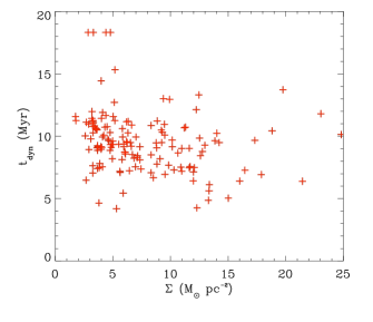
Figure 7: The dynamical time of individual bound entities is plotted against the surface density for the 500 pc² regions in which they lie from Model B, where the mean surface density is 8 M_⊙ pc^-2. Thus although the dynamical time of each bound clump is related to the density of a localised clump of bound gas, this relation largely disappears when considering the dynamical times of all the bound gas clumps in a 500 pc² region.

3.4.3 A change in slope

For plots of the total surface density, we find a change in the slope around 10 M_⊙ pc². Krumholz et al. (2008) interpret this as the surface density at which gas becomes molecular. In our models, this surface density corresponds roughly to the density at which the surface densities of bound and unbound gas are approximately equal. Below this density, the surface density is dominated by low density, unbound gas, and follows a steeper slope, as indicated by the low density criterion on Fig. 6. Above this density, the gas is predominantly bound, thus follows the shallower path. Since the gas generally is self-gravitating at densities high enough for molecular gas to be observable (Hartmann et al., 2001), our critical density is similar to that of Krumholz et al. (2008).

3.4.4 Higher surface densities

A major disadvantage of the analysis presented in this paper is that, for computational reasons, we are unable to include very high surface densities, with no points over $100$ M_⊙ pc^-2. Thus, for example, unlike previous theories and observations (Kennicutt, 1989; Krumholz & McKee, 2005), we are not able to claim applicability of our findings to starbursts.

Our simple analysis in Section 3.2.4 suggests that the star formation rate depends linearly on local surface density, once the gas becomes fully molecular. Whilst a linear relation is observed for molecular gas measured using CO in normal galaxies (Bigiel et al., 2008), it is not clear that this is the case for starbursts. Although Gao & Solomon (2004b) find a linear relation between star formation rate and luminosity in starbursts for $L(HCN)$, they observe that the star formation rate varies with CO flux as $L(CO)^{1.4}$.

Nevertheless, we speculate here that our simple ideas might even be relevant to the high gas surface densities, provided that for these HCN is a better indicator of molecular gas mass than CO. Indeed, various authors (e.g Gao & Solomon 2004a; Wu et al. 2005; Aalto 2008) have noted that CO is not a particularly good tracer of star formation in starbursts compared to HCN. We give two reasons why this might be so.

First, the ¹²CO predominantly traces warm molecular envelopes surrounding cold clouds (Meier et al., 2000; Glenn & Hunter, 2001; Gao & Solomon, 2004b). The ISM in starbursts is also considerably more turbulent than that in normal galaxies (Aalto et al., 1995). Thus it is not implausible to suppose that a substantially smaller fraction of the CO represents self-gravitating gas. Compared to our interpretation of the Bigiel et al. (2008) results in Section 3.4.2, it may be that for starbursts we should regard CO as a proxy for HI and HCN as a proxy for H₂.

Second, it seems plausible to assume expect that at high surface densities optical depth effects start to undermine a simple relation between L(CO) and L(HCN) and surface density. However, it is the CO observations which are likely to be effected first. Thus it may be that at high surface densities, L(CO) underestimates the mass relative to L(HCN).

3.5 Star formation rate versus shock strength

If, as suggested by Roberts (1969), star formation is triggered by spiral density waves, a higher degree of star formation might be expected in galaxies with stronger shocks. This has been the subject of much past debate. Elmegreen & Elmegreen (1986) argued that since grand design spirals do not show an increased star formation rate compared to flocculent galaxies, spiral triggering of star formation is not significant. Instead the gas and thus the star formation is merely arranged into spiral arms. Though some recent observations show that there is a correlation between the SFR and spiral shock strength Seigar & James (2002).

For a stronger spiral potential, the stronger shock leads to more gas in the spiral arms and higher gas densities in the spiral shock. Therefore we may expect that the amount of bound gas increases with shock strength. Fig. 8 shows the star formation rate versus the strength of the spiral potential. The star formation rate does not show an increase with shock strength (within a factor of 2 or 3), but instead remains fairly flat. Thus a stronger shock does not appear to produce a higher star formation rate (averaged over the disc).

The amount of bound gas depends primarily on the density of the gas and on the velocity dispersion. Thus a possible explanation for the apparently constant star formation rate is that the kinetic energy of the dense gas also increases with the strength of the shock. To test this, we plot the velocity dispersion of the clumps in Fig. 9, against the mass of the clumps. The clumps in the higher shock models clearly have a higher velocity dispersion. Thus although they have higher densities, there is not a substantially greater mass of bound gas. However the bound gas is more concentrated to the spiral arms at higher shock strengths, and therefore there is a somewhat higher star formation rate in the spiral arms at higher shock strengths (see Section 3.6).

We illustrate the velocity dispersion increase further in Fig. 10, where the velocity dispersion is plotted against azimuth. The particles used to calculate the dispersion are selected from a ring of width 200 pc at a radius of 7.5 kpc. The velocity dispersion of the gas in the spiral arms generally increases as the shock becomes stronger.

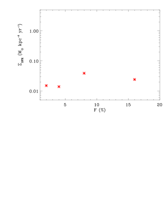
Figure 8: The estimated star formation rate is shown versus the strength of the spiral potential when $\Sigma=4$ M_⊙ pc^-2 (Models A, E, F and G). The star formation remains fairly constant as the strength of the potential increases.

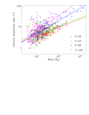
Figure 9: The velocity dispersion is shown against mass for each bound clump, from the simulations with different shock strengths. The velocity dispersions exhibit higher values at higher shock strengths. Best fit lines are also shown through each set of points to illustrate that they are offset.

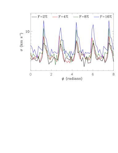
Figure 10: The velocity dispersion is plotted against azimuth for the calculation with different shock strengths. The velocity dispersion becomes greater in the spiral shock as the strength of the shock increases.

3.6 Star formation in spiral arm and interarm regions

As described above, the star formation rate, or mass of bound gas, increases with surface density, but does not vary significantly with spiral shock strength. Here we investigate whether the degree of star formation in the spiral arms compared to inter-arm regions varies according to surface density or shock strength. Gas within a 1 kpc wide extent covering the spiral arms is assumed to be spiral arm material. Figure 11 shows the percentage of bound gas in the spiral arms versus surface density (blue crosses) and the strength of the potential (red diamonds). In these simulations, between 65 and 90 per cent of the bound gas is located in the spiral arms. The percentage of bound gas in the spiral arms decreases with surface density. This indicates that at lower mean surface densities, the self-gravity of the gas becomes more important compared to the strength of the shock. Possibly at high surface densities, gravitational instabilities lead to bound gas in the interarm regions. However the greatest contribution to the interarm bound gas is from gas which has become bound in the spiral arms, and remains mainly bound in the interarm region.

The percentage of bound gas which is located in the arms increases with spiral shock strength. Thus a higher degree of star formation is likely to occur in the spiral arms for the models with a stronger spiral potential. Though as discussed in the previous section, the total star formation rate does not change significantly, instead as suggested by Elmegreen & Elmegreen (1986), there is more star formation in the spiral arms simply because more of the gas is there.

The mass of bound gas is calculated using the kinetic, thermal and magnetic energies. If only the kinetic energy is used, comparatively more bound gas lies in the interarm regions. However the trends shown on Fig. 11 do not change.

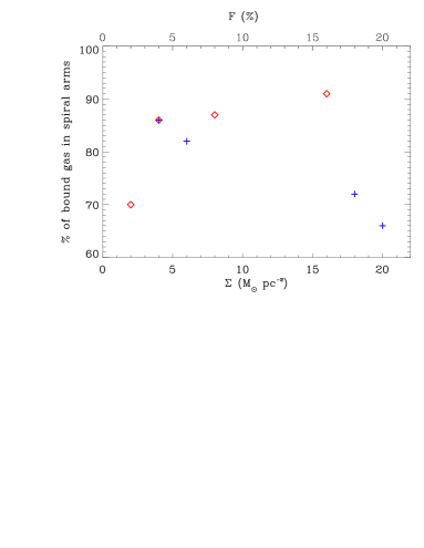
Figure 11: The percentage of bound gas which lies in the spiral arms is plotted against surface density (blue crosses) and against strength of the potential (red diamonds). At higher surface densities, self gravity becomes more important relative to the strength of the shock, and less of the bound gas lies in the spiral arms. As the strength of the potential increases though (and thus the strength of the spiral shock), more of the bound gas lies in the spiral arms.

4 Conclusions

We have investigated the degree to which the relationship between the star formation rate per unit area and the surface density of the ISM in a star-forming galaxy can be understood in terms of simple input assumptions.

We model the ISM as a self-gravitating, two-phase medium, with one half the mass at a fixed cool temperature of $T=100$K, as a proxy for H₂, and the other half at a fixed warm temperature $T=10^{4}$K, as a proxy for Hi. We estimate (Section 2.2) the local star formation rate in a bound clump as being the mass of the clump divided by its dynamical timescale, multiplied by an efficiency factor $\epsilon$ which we take to be $\epsilon=0.05$ to give a fit to the observations.

Using these simple input assumptions we find that we can reproduce the observed relationship which indicates that the local star formation rate per unit area is linearly proportional to the local surface density of dense gas (Figure 6). We show that this direct linear proportionality comes about because (Figure 7) the local dynamical timescales of bound entities do not correlate with local mean surface densities.

We also show, in agreement with the observations, that the total surface density (being a proxy for $\Sigma(HI+H_{2})$) and the surface density of warm gas (being a proxy for $\Sigma(HI)$) are not good indicators of local star formation rates. A simple model (Section 3.4.2) for the dependence of H₂ fraction, $f(H_{2})$, as a function of total surface density, in the regime where $f(H_{2})<1$, provides a simple explanation of why the surface star formation rate is a steeper function of total surface density in this regime. Moreover, it is evident from this simple model that the star formation rate does not have a one-to-one relationship with Hi surface density, implying that any attempt to correlate star formation rates with Hi surface density is likely to result in large scatter.

We are also able to demonstrate from these simple considerations that the star formation rate averaged over the galaxy disc does not depend significantly on the strength of the spiral shock (Figure 8). This is because, although a stronger shock does result in a higher gas density downstream of the shock, it also results in a higher dispersion velocity (Figures 9 and 10). A stronger shock does, however, result in more of the bound gas, and therefore more of the star formation lying close to the spiral arms.

References

- Aalto (2008) Aalto S., 2008, Ap&SS, 313, 273
- Aalto et al. (1995) Aalto S., Booth R. S., Black J. H., Johansson L. E. B., 1995, A&A, 300, 369
- Agertz et al. (2009) Agertz O., Lake G., Teyssier R., Moore B., Mayer L., Romeo A. B., 2009, MNRAS, 392, 294
- Bate (1995) Bate M., 1995, PhD thesis, Univ. Cambridge
- Bigiel et al. (2008) Bigiel F., Leroy A., Walter F., Brinks E., de Blok W. J. G., Madore B., Thornley M. D., 2008, AJ, 136, 2846
- Binney & Tremaine (1987) Binney J., Tremaine S., 1987, Galactic dynamics. Princeton, NJ, Princeton University Press, 1987, 747 p.
- Booth et al. (2007) Booth C. M., Theuns T., Okamoto T., 2007, MNRAS, 376, 1588
- Bottema (2003) Bottema R., 2003, MNRAS, 344, 358
- Caldwell & Ostriker (1981) Caldwell J. A. R., Ostriker J. P., 1981, ApJ, 251, 61
- Cox & Gómez (2002) Cox D. P., Gómez G. C., 2002, ApJS, 142, 261
- Dobbs (2008) Dobbs C. L., 2008, MNRAS, 391, 844
- Dobbs et al. (2008) Dobbs C. L., Glover S. C. O., Clark P. C., Klessen R. S., 2008, MNRAS, 389, 1097
- Elmegreen (2002) Elmegreen B. G., 2002, ApJ, 577, 206
- Elmegreen & Elmegreen (1986) Elmegreen B. G., Elmegreen D. M., 1986, ApJ, 311, 554
- Gao & Solomon (2004a) Gao Y., Solomon P. M., 2004a, ApJS, 152, 63
- Gao & Solomon (2004b) Gao Y., Solomon P. M., 2004b, ApJ, 606, 271
- Glenn & Hunter (2001) Glenn J., Hunter T. R., 2001, ApJS, 135, 177
- Gnedin et al. (2008) Gnedin N. Y., Tassis K., Kravtsov A. V., 2008, ArXiv e-prints
- Hartmann et al. (2001) Hartmann L., Ballesteros-Paredes J., Bergin E. A., 2001, ApJ, 562, 852
- Heyer et al. (2004) Heyer M. H., Corbelli E., Schneider S. E., Young J. S., 2004, ApJ, 602, 723
- Hou et al. (2000) Hou J. L., Prantzos N., Boissier S., 2000, A&A, 362, 921
- Kennicutt (1989) Kennicutt R. C., 1989, ApJ, 344, 685
- Kennicutt (1998) Kennicutt R. C., 1998, ARA&A, 36, 189
- Kennicutt & et. al. (2007) Kennicutt Jr. R. C., et. al. 2007, ApJ, 671, 333
- Krumholz & McKee (2005) Krumholz M. R., McKee C. F., 2005, ApJ, 630, 250
- Krumholz et al. (2008) Krumholz M. R., McKee C. F., Tumlinson J., 2008, ApJ, 689, 865
- Krumholz & Tan (2007) Krumholz M. R., Tan J. C., 2007, ApJ, 654, 304
- Krumholz & Thompson (2007) Krumholz M. R., Thompson T. A., 2007, ApJ, 669, 289
- Li et al. (2006) Li Y., Mac Low M.-M., Klessen R. S., 2006, ApJ, 639, 879
- Meier et al. (2000) Meier D. S., Turner J. L., Hurt R. L., 2000, ApJ, 531, 200
- Roberts (1969) Roberts W. W., 1969, ApJ, 158, 123
- Robertson & Kravtsov (2008) Robertson B. E., Kravtsov A. V., 2008, ApJ, 680, 1083
- Saitoh et al. (2008) Saitoh T. R., Daisaka H., Kokubo E., Makino J., Okamoto T., Tomisaka K., Wada K., Yoshida N., 2008, PASJ, 60, 667
- Schmidt (1959) Schmidt M., 1959, ApJ, 129, 243
- Schuster et al. (2007) Schuster K. F., Kramer C., Hitschfeld M., Garcia-Burillo S., Mookerjea B., 2007, A&A, 461, 143
- Seigar & James (2002) Seigar M. S., James P. A., 2002, MNRAS, 337, 1113
- Shetty & Ostriker (2008) Shetty R., Ostriker E. C., 2008, ApJ, 684, 978
- Silk (1997) Silk J., 1997, ApJ, 481, 703
- Springel (2000) Springel V., 2000, MNRAS, 312, 859
- Springel & Hernquist (2003) Springel V., Hernquist L., 2003, MNRAS, 339, 289
- Susa (2008) Susa H., 2008, ApJ, 684, 226
- Tan (2000) Tan J. C., 2000, ApJ, 536, 173
- Tan et al. (1999) Tan J. C., Silk J., Balland C., 1999, ApJ, 522, 579
- Tasker & Bryan (2006) Tasker E. J., Bryan G. L., 2006, ApJ, 641, 878
- Tasker & Bryan (2008) Tasker E. J., Bryan G. L., 2008, ApJ, 673, 810
- Tasker & Tan (2008) Tasker E. J., Tan J. C., 2008, ArXiv e-prints
- van den Bosch (2000) van den Bosch F. C., 2000, ApJ, 530, 177
- Wong & Blitz (2002) Wong T., Blitz L., 2002, ApJ, 569, 157
- Wu et al. (2005) Wu J., Evans II N. J., Gao Y., Solomon P. M., Shirley Y. L., Vanden Bout P. A., 2005, ApJL, 635, L173
- Wyse (1986) Wyse R. F. G., 1986, ApJL, 311, L41
- Wyse & Silk (1989) Wyse R. F. G., Silk J., 1989, ApJ, 339, 700