Effective permittivity of mixtures of anisotropic particles

Abstract

We use a new approach to derive dielectric mixing rules for macroscopically homogeneous and isotropic multicomponent mixtures of anisotropic inhomogeneous dielectric particles. Two factors of anisotropy are taken into account, the shape of the particles and anisotropy of the dielectric parameters of the particles’ substances. Our approach is based upon the notion of macroscopic compact groups of particles and the procedure of averaging of the fields over volumes much greater than the typical scales of these groups. It enables us to effectively sum up the contributions from multiple interparticle reemission and short-range correlation effects, represented by all terms in the infinite iterative series for the electric field strength and induction. The expression for the effective permittivity can be given the form of the Lorentz-Lorenz type, which allows us to determine the effective polarizabilities of the particles in the mixture. These polarizabilities are found as integrals over the regions occupied by the particles and taken of explicit functions of the principal components of the permittivity tensors of the particles’ substances and the permittivity of the host medium. The case of a mixture of particles of the ellipsoidal shape is considered in detail to exemplify the use of general formulas. As another example, Bruggeman-type formulas are derived under pertinent model assumptions. The ranges of validity of the results obtained are discussed as well.

I INTRODUCTION

The study of effective permittivity of heterogeneous systems holds an important position in various fields of physics and technics, for its results find wide-spread applications in composite material engineering, biochemical technology, medical diagnostics, etc. In theoretical research, the simplest and much discussed model considers a heterogeneous system as a mixture of fine particles of the disperse phase embedded into a continuous host medium. The development of it began with the case of dilute mixtures of small spherical inclusions more than century ago bib:MGarnett1904 and has resulted, in particular, in the classical Maxwell-Garnett (MG) mixing rule and its various modifications (see Ref. bib:Brosseau2006, for an analysis of relevant physical concepts and ideas from a historical perspective, and Refs. bib:Bohren1983, ; bib:Sihvola1999, ; bib:Tsang2001, for a review of major results). It has been shown so far that: (1) The MG formula can incorporate multiple scattering effects (see, for instance, analytical results bib:Claro1991 ; bib:Fu1993 obtained in the quasistatic limit within a mean-field approximation). (2) For certain configurations of the disperse particles, it remains accurate for high-concentrated mixtures, bib:Abeles1976 ; bib:Spanoudaki2001 ; bib:Wu2001 ; bib:Robinson2002 ; bib:Mallet2005 in which strong electromagnetic interaction is significant and for which another – the Bruggeman mixing rule bib:Bruggeman1935 – is often believed to be superior to the former.

The case of mixtures of anisotropic particles remains little-investigated (see reviews, bib:Sihvola1999 ; bib:Tsang2001 after whose appearance the state of the art has not changed much). As far as we know, the existing attempts at taking the particles’ anisotropy into account usually reduce to or heavily rely on different kinds of one-particle approximations, including their combinations (see, for instance, Refs. bib:Levy1997, ; bib:Jilha2007, and references therein). A typical example of such approximations is the use of the one-particle polarizability, describing the response of a solitary particle to a uniform electric field, instead of the effective polarizability of the particle in the mixture. It is evident that such an approach is tolerable only for diluted gases of anisotropic particles. In sufficiently concentrated mixtures, both multiple polarization effects and many-particle correlations in positions and orientations of the particles come into play. As a result, finding the effective polarizability becomes a many-particle problem, which is equivalent to the original problem of finding the effective permittivity of the mixture. Correspondingly, neither the effective polarizability as a function of the dielectric and geometric parameters of disperse particle, nor the interrelation of the two factors of anisotropy of the particles – nonsphericity of the shape and anisotropy of the substance – can be determined consistently within a one-particle approximation. Yet we are unaware of any practically important attempts at approaching these problems using the methods of multiple-scattering theory (in contrast to the case of spherical inclusions, for which see review, bib:Tsang2001 key works, bib:Lax1952 ; bib:Lamb1980 ; bib:Tsang1980 ; bib:Davis1985 and Refs. bib:Mallet2005, ; bib:Kuzmin2005, ). This fact is readily explained by the lack of knowledge of an infinite set of the correlation functions for concentrated systems of anisotropic particle. Even if such information were available, practical calculations would be extremely difficult and would probably be limited to estimations of several corrections to the Born approximation.

Recently, bib:Sushko2007 we proposed a new approach to analysis of the long-wavelength value of the effective permittivity of finely dispersed mixtures. The idea was to avoid excessive theoretical refining on polarization and correlation processes that occur within the system on particle-size and interparticle-distance scales by averaging their contributions out over macroscopic regions reproducing the properties of the entire system. The appropriate procedure is based upon the notion of macroscopic compact groups of particles and the averaging bib:LandauV8 of fields over volumes much greater than the typical scales of these groups. By applying it, we carried out bib:Sushko2007 a rigorous analysis of the effective permittivity of a concentrated mixture of spherically symmetric dielectric balls with piecewise-continuous radial permittivity profile. Later, bib:Sushko2009 the method was applied to systems comprising nonspherical inclusions with scalar permittivity. It was also shown that both the MG and Bruggeman mixing rules can be reconstructed with it.

In the present report, approach bib:Sushko2007 is developed for macroscopically homogeneous and isotopic mixtures of anisotropic dielectric particles whose dielectric properties are described by permittivity tensors and which are embedded in a host medium with constant scalar permittivity; the particles are assumed to be hard, measurable, and, in general, inhomogeneous. It is shown that the averaged contributions from all-order reemission and short-range correlation effects within such a system can be effectively summed up. As a result, the effective static permittivity of the system is obtained as an explicit function of the parameters of the model. It can be given the form of the Lorentz-Lorenz type, the polarization properties of the particles being characterized by their effective polarizabilities in the mixture. The latter are found via the geometric and dielectric parameters of the particles and the host medium; as an example, a mixture of particles of the ellipsoidal shape is considered in detail. Finally, Bruggeman-type formulas are shown to follow from the general formulas under special choices of the effective medium, and the ranges of validity of the results obtained are discussed.

II BASIC RELATIONS FOR ELECTRIC FIELD AND INDUCTION

To begin with, we consider the problem on propagation of electromagnetic waves in a finely dispersed mixture with local permittivity $\varepsilon_{ik}({\rm{\bf r}})=\varepsilon_{0}\delta_{ik}+\delta\varepsilon_{ik}({\rm{\bf r}})$. Here, $\varepsilon_{0}$ is the permittivity of the host medium and $\delta\varepsilon_{ik}({\rm{\bf r}})$ is the contribution caused by compact groups of the disperse anisotropic particles. By a compact group we understand any macroscopic region within which all interparticle distances $|{\rm{\bf r}}_{\lambda}-{\rm{\bf r}}_{\mu}|$ are small as compared to the wavelength of the probing wave in the mixture: $\sqrt{\varepsilon_{0}}k_{0}|{\rm{\bf r}}_{\lambda}-{\rm{\bf r}}_{\mu}|<<1$, where $k_{0}$ is the wave vector of the wave in vacuum (see Fig. 1).

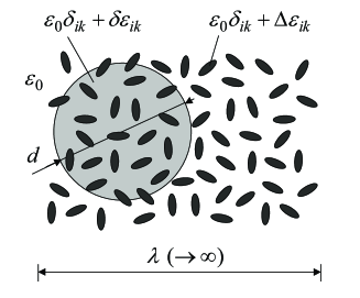
Figure 1: Homogenization of a mixture in terms of compact groups, viewed as macroscopic many-particle regions with linear sizes $d$ much less than the wavelength $\lambda$ of probing radiation.

According to Ref. bib:Sushko2007, , we expect that it is multiple reemission and short-range correlation effects within such groups that form the effective permittivity of the mixture in the static limit $\sqrt{\varepsilon_{0}}k_{0}\to 0$, where even quite large groups of disperse particles become compact. With respect to an external static field, such groups can actually be treated as point-like; fluctuations of macroscopically large numbers of particles contained in them, as well as correlations between the groups, can be ignored. Correspondingly, the deviation $\delta\varepsilon_{ik}({\rm{\bf r}})$ of the local permittivity in the mixture from the permittivity of the host due to the presence at the point r of a compact group of $N$ identical disperse particles, occupying measurable regions ${\rm\Omega}_{\lambda}$ with individual volumes $v$, can be modelled as

$$\delta\varepsilon_{ik}({\rm{\bf r}})={\sum\limits_{\lambda=1}^{N}{\Delta\varepsilon_{ik}({\rm{\bf r}},{\rm\Omega}_{\lambda})\,\Pi({\rm{\bf r}},{\rm\Omega}_{\lambda})}},$$ (1)

where $\Delta\varepsilon_{ik}({\rm{\bf r}},{\rm\Omega}_{\lambda})=\varepsilon_{ik}({\rm{\bf r}},{\rm\Omega}_{\lambda})-\varepsilon_{0}\delta_{ik}$ is the deviation of the local permittivity in the mixture from the permittivity of the host due to the presence of the $\lambda$th particle at r, $\varepsilon_{ik}({\rm{\bf r}},{\rm\Omega}_{\lambda})$ stands for the permittivity tensor of the substance of this particle, $\Pi({\rm{\bf r}},{\rm\Omega}_{\lambda})$ is the characteristic function of the region ${\rm\Omega}_{\lambda}$ [$\Pi({\rm{\bf r}},{\rm\Omega}_{\lambda})=1$ if $\textbf{r}\in{\rm\Omega}_{\lambda}$ and $\Pi({\rm{\bf r}},{\rm\Omega}_{\lambda})=0$ otherwise], and $\delta_{ik}$ is the Kronecker delta. In what follows, the tensors $\delta\varepsilon_{ik}({\rm{\bf r}})$, $\varepsilon_{ik}({\rm{\bf r}},{\rm\Omega}_{\lambda})$, and $\Delta\varepsilon_{ik}({\rm{\bf r}},{\rm\Omega}_{\lambda})$ will also be designated as $\hat{\mathop{\delta\varepsilon}}$, $\hat{\mathop{\varepsilon}}$, and $\hat{\mathop{\Delta\varepsilon}}$ respectively.

The equation for the $i$ component of the electric field of a wave in the mixture can be written as bib:LandauV8

$$\Delta E_{i}+k_{0}^{2}\varepsilon_{0}E_{i}-\nabla_{i}\nabla_{k}E_{k}=-k_{0}^{2}\delta\varepsilon_{ik}{\kern 1.0pt}E_{k};$$ (2)

henceforth, the dummy suffix convention applies. Eq. (2) is equivalent to the integral equation

$$E_{i}({\rm{\bf r}})=E_{i}^{(0)}({\rm{\bf r}})-k_{0}^{2}{\int\limits_{V}{d{\rm{\bf{r}^{\prime}}}\,T_{ij}({\rm{\bf r}},{\rm{\bf{r}^{\prime}}})\delta\varepsilon_{jk}({\rm{\bf{r}^{\prime}}})E_{k}({\rm{\bf{r}^{\prime}}})}},$$ (3)

where $E_{i}^{(0)}({\rm{\bf r}})=E_{i}^{0}\exp\left({i\sqrt{\varepsilon_{0}}{\rm{\bf k}}_{0}\cdot{\rm{\bf r}}}\right)$ is the $i$ component of the incident wave field in the mixture, $E_{i}^{0}$ is the $i$ component of the field amplitude ${\rm{\bf E}}_{0}$, and $T_{ij}(r)={{-\left({k_{0}^{2}\delta_{ij}+\nabla_{i}\nabla_{j}}\right)\exp\left({ik_{0}\sqrt{\varepsilon_{0}}}r\right)}\mathord{\left/{\vphantom{{-\left({k_{0}^{2}\delta_{ij}+\nabla_{i}\nabla_{j}}\right)\exp\left({{i}k_{0}\sqrt{\varepsilon_{0}}}\right)}{4\pi k_{0}^{2}\varepsilon_{0}r}}}\right.\kern-1.2pt}{4\pi k_{0}^{2}\varepsilon_{0}r}}$ are the components of the electromagnetic field propagator [Green’s tensor for Eq. (3)]; the integral in Eq. (3) is taken over the volume of the mixture.

With the iterative procedure applied, the solution of Eq. (3) can be represented in the form

$$E_{i}({\rm{\bf r}})=E_{i}^{(0)}({\rm{\bf r}})+{\sum\limits_{n=1}^{\infty}{E_{i}^{(n)}({\rm{\bf r}})}},$$ (4)

$$E_{i}^{(n)}({\rm{\bf r}})=(-k_{0}^{2})^{n}{\int\limits_{V}{d{\rm{\bf r}}_{1}}}{\int\limits_{V}{d{\rm{\bf r}}_{2}}}\ldots{\int\limits_{V}{d{\rm{\bf r}}_{n}}}\,T_{ij}({\rm{\bf r}},{\rm{\bf r}}_{1})\delta\varepsilon_{jk}({\rm{\bf r}}_{1})$$

$$\times T_{kl}({\rm{\bf r}}_{1},{\rm{\bf r}}_{2})\delta\varepsilon_{lm}({\rm{\bf r}}_{2})\ldots T_{rs}({\rm{\bf r}}_{n-1},{\rm{\bf r}}_{n})\delta\varepsilon_{st}({\rm{\bf r}}_{n})E_{t}^{(0)}({\rm{\bf r}}_{n}).$$

(5)

The $i$ component of the electric induction vector at the point ${\rm{\bf r}}$ in the mixture is given by

$$D_{i}({\rm{\bf r}})={\left[{\varepsilon_{0}\delta_{ik}+\delta\varepsilon_{ik}({\rm{\bf r}})}\right]}\,E_{k}({\rm{\bf r}}).$$ (6)

Assuming that the mixture as a whole is macroscopically homogenous and isotropic, we define its effective permittivity $\varepsilon_{\rm eff}$ in the standard way, bib:LandauV8 as the proportionality coefficient in the relation

$$\overline{{D}_{i}}=\varepsilon_{\rm eff}{\kern 1.0pt}\overline{{E}_{i}},$$ (7)

where the bars indicate averaging by the rule $\overline{{A}_{i}}={\frac{{1}}{{V}}}{\int\limits_{V}{A_{i}({\rm{\bf r}}){\kern 1.0pt}d{\rm{\bf r}}}}$; the volume $V$ is implied to be much greater than the volumes of compact groups. Following Ref. bib:LandauV8, , we accept that for finely dispersed mixtures, the values $\overline{{A}_{i}}$ are equal to the corresponding statistical averages ${\left\langle{A_{i}({\rm{\bf r}})}\right\rangle}$ over the positions and orientations of disperse particle.

Now, under the suggestions made, we can prove quantitatively the following two statements: (1) In the limiting case $\sqrt{\varepsilon_{0}}k_{0}\to 0$, the values ${\kern 1.0pt}\overline{{E}_{i}}$ and $\overline{{D}_{i}}$ are determined only by the multiple reemission and short-range correlation effects inside compact groups. (2) The corresponding all-order contributions to $\varepsilon_{\rm eff}$ can be singled out from the iterative series by formal replacing the factors $k_{0}^{2}T_{ij}(r)$ in the integrals for ${\kern 1.0pt}\overline{{E}_{i}}$ and $\overline{{D}_{i}}$ with the expressions ${{\delta({\rm{\bf r}})\delta_{ij}}\mathord{\left/{\vphantom{{\delta({\rm{\bf r}})\delta_{ij}}{3\varepsilon_{0}}}}\right.\kern-1.2pt}{3\varepsilon_{0}}}$, where $\delta({\rm{\bf r}})$ is the Dirac delta function. This replacement simply reflects the fact that within a macroscopic approach, the specified contributions are formed by those ranges of the integration variables where the electromagnetic field propagators reveal a singular behavior.

Our proof uses the representation bib:LandauV4

$${\mathop{\lim}\limits_{k_{0}\to 0}}k_{0}^{2}{\tilde{T}}_{ij}({\rm{\bf r}})=-{\frac{{1}}{{4\pi\varepsilon_{0}}}}\nabla_{i}\nabla_{j}{\frac{{1}}{{r}}}$$

$$={\frac{{1}}{{3\varepsilon_{0}}}}\delta_{ij}\delta({\rm{\bf r}})+{\frac{{1}}{{4\pi\varepsilon_{0}r^{3}}}}\left({\delta_{ij}-3e_{i}e_{j}}\right)$$ (8)

for the propagator $T_{ij}({\rm{\bf r}})$, which is valid (see Ref. bib:Sushko2004, for mathematical details) on a set of scalar, compactly supported, and bounded functions $\delta\varepsilon_{\alpha\beta}({\rm{\bf r}})$ in the sense that there holds the relation

$${\mathop{\lim}\limits_{k_{0}\to 0}}{\int\limits_{V}{d{\rm{\bf r}}}}k_{0}^{2}T_{ij}({\bf{r}})\delta\varepsilon_{\alpha\beta}({\rm{\bf r}})={\mathop{\lim}\limits_{k_{0}\to 0}}{\int\limits_{V}{d{\rm{\bf r}}}}k_{0}^{2}{\tilde{T}}_{ij}({\bf{r}})\delta\varepsilon_{\alpha\beta}({\rm{\bf r}}).$$

In Eq. (8), $e_{i}$ stands for the $i$ component of the unit vector ${\rm{\bf e}}={{{\rm{\bf r}}}\mathord{\left/{\vphantom{{{\rm{\bf r}}}{r}}}\right.\kern-1.2pt}{r}}$; for brevity, the first and the second terms to the right of the equality sign will also be denoted by $\hat{\tau}^{(1)}$ and $\hat{\tau}^{(2)}$ respectively.

With the aid of (8), the contribution to the statistical average ${\left\langle{E_{i}({\rm{\bf r}})}\right\rangle}$ from the $n$th iterative step can be represented in the static limit $\sqrt{\varepsilon_{0}}k_{0}\to 0$ as

$${\left\langle{E_{i}^{(n)}({\rm{\bf r}})}\right\rangle}={\left\langle{E_{i}^{(n;1)}({\rm{\bf r}})}\right\rangle}+{\left\langle{E_{i}^{(n;1,2)}({\rm{\bf r}})}\right\rangle}.$$ (9)

The addend

$${\left\langle{E_{i}^{(n;1)}({\rm{\bf r}})}\right\rangle}=\left({-{\frac{{1}}{{3\varepsilon_{0}}}}}\right)^{n}{\left\langle{\delta\varepsilon_{ik}({\rm{\bf r}})\delta\varepsilon_{km}({\rm{\bf r}})\ldots\delta\varepsilon_{rt}({\rm{\bf r}})}\right\rangle}E_{t}^{0}$$ (10)

represents the statistical average of a product of $n$ factors $\hat{\mathop{\delta\varepsilon}}$ related to a single compact group; it is obtained by replacing all factors $k_{0}^{2}\hat{T}$ in (5) by the their most singular parts $\hat{\tau}^{(1)}$. The addend ${\left\langle{E_{i}^{(n;1,2)}({\rm{\bf r}})}\right\rangle}$ is the sum of all integrals containing at least one factor $\hat{\tau}^{(2)}$ under the integral sign. Each expression containing $m\leq n$ factors of the $\hat{\tau}^{(2)}$ type results from taking $(n-m)$ integrals with $\hat{\tau}^{(1)}$ factors in their integrands; it is therefore proportional to the expression

$${\int\limits_{V}{d{\rm{\bf r}}_{1}}}{\int\limits_{V}{d{\rm{\bf r}}_{2}}}\ldots{\int\limits_{V}{d{\rm{\bf r}}_{m}}}\,\hat{\tau}^{(2)}\left({{\rm{\bf r}}-{\rm{\bf r}}_{1}}\right)\hat{\tau}^{(2)}\left({{\rm{\bf r}}_{1}-{\rm{\bf r}}_{2}}\right)\ldots\hat{\tau}^{(2)}\left({{\rm{\bf r}}_{m-1}-{\rm{\bf r}}_{m}}\right)$$

$$\times{\left\langle{\left({\hat{\mathop{\delta\varepsilon}}({\rm{\bf r}}_{1})}\right)^{i_{1}}\left({\hat{\mathop{\delta\varepsilon}}({\rm{\bf r}}_{2})}\right)^{i_{2}}\ldots\left({\hat{\mathop{\delta\varepsilon}}({\rm{\bf r}}_{m})}\right)^{i_{m}}}\right\rangle}{\rm{\bf E}}^{0},$$

where $i_{1}+i_{2}+...+i_{m}=n$. Since the spacial and orientational correlations between macroscopic compact groups in a macroscopically homogeneous and isotropic mixture are negligibly small, the many-point (involving different compact groups) correlator in this expression can be factorized as a product of one-point correlators, each of which is related to a single compact group. The one-point correlators are equal to linear combinations of expressions constructed of Kronecker deltas and satisfying certain symmetry constraints on permutations of their indices. In particular, the average ${\left\langle{\delta\varepsilon_{jk}({\rm{\bf r}}_{1})}\right\rangle}=A\delta_{jk}$ is symmetric with respect to permutations $j\leftrightarrow k$, the average ${\left\langle{\delta\varepsilon_{jk}({\rm{\bf r}}_{1})\delta\varepsilon_{lm}({\rm{\bf r}}_{1})}\right\rangle}=B\delta_{jk}\delta_{lm}+C\left({\delta_{jl}\delta_{km}+\delta_{jm}\delta_{kl}}\right)$ is symmetric with respect to permutations $j\leftrightarrow k$, $l\leftrightarrow m$ of individual indices and permutations $(j,k)\leftrightarrow(l,m)$ of their pairs, etc. The coefficients $A$, $B$, $C,\ldots$ in these relations depend on the physical parameters of the host and disperse particles, but not on the coordinates of the relevant compact group. As a consequence, the integrals in ${\left\langle{E_{i}^{(n;1,2)}({\rm{\bf r}})}\right\rangle}$ reduce to those taken of factors $\hat{\tau}^{(2)}$ alone. Taking into account the explicit form of $\hat{\tau}^{(2)}$, we see that these integrals vanish after integration with respect to the angles. Thus,

$${\left\langle{E_{i}^{(n;1,2)}({\rm{\bf r}})}\right\rangle}=0.$$ (11)

In view of the equality of the averages ${\left\langle{E_{i}({\rm{\bf r}})}\right\rangle}$ and $\overline{{E}_{i}}$, Eqs. (9)–(11) give

$$\overline{\mathop{E_{i}^{(n)}({\rm{\bf r}})}}=\left({-{\frac{{1}}{{3\varepsilon_{0}}}}}\right)^{n}\overline{\mathop{\delta\varepsilon_{ik}({\rm{\bf r}})\delta\varepsilon_{km}({\rm{\bf r}})\ldots\delta\varepsilon_{rt}({\rm{\bf r}})}}E_{t}^{0}.$$ (12)

Similar reasoning is used to analyze the averages ${\left\langle{D_{i}({\rm{\bf r}})}\right\rangle}$ and $\overline{{D}_{i}}$. From Eqs. (4)–(6), we finally obtain:

$$\overline{{E}_{i}}=\left[\delta_{it}+\sum\limits_{\sigma=1}^{\infty}\left(-\frac{1}{3\varepsilon_{0}}\right)^{\sigma}\overline{\mathop{\delta}\varepsilon_{ik}({\rm\bf r})\delta\varepsilon_{km}({\rm\bf r})\ldots\delta\varepsilon_{rt}({\rm\bf r})}\right]E_{t}^{0},$$ (13)

$$\overline{{D}_{i}}={\left[\varepsilon_{0}\delta_{it}+\varepsilon_{0}{\sum\limits_{\sigma=1}^{\infty}\left({-{\frac{{1}}{{3\varepsilon_{0}}}}}\right)^{\sigma}\overline{\mathop{\delta\varepsilon_{ik}({\rm{\bf r}})\delta\varepsilon_{km}({\rm{\bf r}})\ldots\delta\varepsilon_{rt}({\rm{\bf r}})}}}\right.}$$

$$+{\left.\sum\limits_{\sigma=0}^{\infty}{\left({-{\frac{{1}}{{3\varepsilon_{0}}}}}\right)^{\sigma}\overline{\mathop{\delta\varepsilon_{ik}({\rm{\bf r}})\delta\varepsilon_{km}({\rm{\bf r}})\ldots\delta\varepsilon_{pr}({\rm{\bf r}})\delta\varepsilon_{rt}({\rm{\bf r}})}}}\right]}E_{t}^{0}.$$ (14)

Note that there are, respectively, $\sigma$ and $\sigma+1$ factors under the bars in the sum from 1 to $\infty$ and that from 0 to $\infty$.

III EFFECTIVE PERMITTIVITY OF MATRIX-PARTICLE MIXTURES

For a macroscopically homogeneous and isotropic mixture, the averages $\overline{{E}_{i}}$ and $\overline{{D}_{i}}$ are proportional to the corresponding component $E_{i}^{0}$ of the external field. Since different terms in series (13) and (14) are independent, it is reasonable to suggest that they have the structure

$$\overline{\mathop{\delta\varepsilon_{ik}({\rm{\bf r}})\delta\varepsilon_{km}({\rm{\bf r}})\ldots\delta\varepsilon_{rt}({\rm{\bf r}})}}=A_{\sigma}\delta_{it},$$ (15)

where the subscript $\sigma$ specifies the number of factors under the bar. The summation over the indices $i=t$ yields

$$A_{\sigma}={\frac{{1}}{{3}}}\overline{{\textrm{Tr}}\,\left({\hat{\mathop{\delta\varepsilon}}({\rm{\bf r}})\,}\right)^{\sigma}}.$$ (16)

This trace is easily found, for in the typical expression

$$\overline{\mathop{\delta\varepsilon_{ik}({\rm{\bf r}})\delta\varepsilon_{km}({\rm{\bf r}})\ldots\delta\varepsilon_{rt}({\rm{\bf r}})}}$$

$$={\sum\limits_{\lambda_{1}=1}^{N}{{\sum\limits_{\lambda_{2}=1}^{N}{\ldots{\sum\limits_{\lambda_{\sigma}=1}^{N}{{\frac{{1}}{{V}}}{\int\limits_{V}{d{\rm{\bf r}}}}\,\Delta\varepsilon_{ik}({\rm{\bf r}},{\rm{\Omega}}_{\lambda_{1}})\Pi({\rm{\bf r}},{\rm{\Omega}}_{\lambda_{1}})}}}}}}$$

$$\times\Delta\varepsilon_{km}({\rm{\bf r}},{\rm{\Omega}}_{\lambda_{2}})\Pi({\rm{\bf r}},{\rm{\Omega}}_{\lambda_{2}})\ldots\Delta\varepsilon_{rt}({\rm{\bf r}},{\rm{\Omega}}_{\lambda_{\sigma}})\Pi({\rm{\bf r}},{\rm\Omega}_{\lambda_{\sigma}})$$

all addends with two and more differing values of the indices $\lambda_{1},\lambda_{2},\ldots,\lambda_{\sigma}$ are zero (the regions occupied by hard particles never overlap). If all of these values are equal, then the relation $[\Pi({\rm{\bf r}},{\rm\Omega}_{\lambda})]^{\sigma}=\Pi({\rm{\bf r}},{\rm\Omega}_{\lambda})$ ($\sigma$ any natural number) gives

$$\overline{\mathop{{\textrm{Tr}}\,\left({\hat{\mathop{\delta\varepsilon}}({\rm{\bf r}})}\right)^{\sigma}}}={\sum\limits_{\lambda=1}^{N}\frac{{1}}{{V}}}{\int\limits_{\Omega_{\lambda}}{d{\rm{\bf r}}}}\,\Delta\varepsilon_{ik}({\rm{\bf r}},{\rm\Omega}_{\lambda})\Delta\varepsilon_{km}({\rm{\bf r}},{\rm\Omega}_{\lambda})\ldots$$

$$\times\Delta\varepsilon_{ri}({\rm{\bf r}},{\rm\Omega}_{\lambda})=n{\int\limits_{v}{d{\rm{\bf r}}}}\,{\textrm{Tr}}\,\left({\hat{\mathop{\Delta\varepsilon}}({\rm{\bf r}},{\rm\Omega}_{\lambda})}\right)^{\sigma}.$$

Here, $n={{N}\mathord{\left/{\vphantom{{N}{V}}}\right.\kern-1.2pt}{V}}$ is the particle concentration, the last integral is taken over the region occupied by a single particle, and the integrands are assumed to be wise-continuous. Thus,

$$A_{\sigma}={\frac{{n}}{{3}}}{\int\limits_{v}{d{\rm{\bf r}}}}\,{\textrm{Tr}}\,\left({\hat{\mathop{\Delta\varepsilon}}({\rm{\bf r}},{\rm\Omega}_{\lambda})}\right)^{\sigma},$$

or, in terms of the principal components $\Delta\varepsilon_{ii}({\bf{r}})$ of $\hat{\mathop{\Delta\varepsilon}}$ ($i=1,\,2,\,3$),

$$A_{\sigma}={\frac{{n}}{{3}}}{\int\limits_{v}{d{\rm{\bf r}}}}{\{{[\Delta\varepsilon_{11}({\rm{\bf r}})]^{\sigma}+[\Delta\varepsilon_{22}({\rm{\bf r}})]^{\sigma}+[\Delta\varepsilon_{33}({\rm{\bf r}})]^{\sigma}\,}\}},\sigma\geq 1.$$ (17)

It follows from Eq. (17) that the field (13) and induction (14) are represented by infinite geometric series. Summing them up and using definition (7), we obtain a formula of the Lorentz–Lorenz type:

$${{\varepsilon_{\rm eff}}}={{\varepsilon_{0}}}{\left({1+{\frac{{8\pi}}{{3}}}n\alpha_{\rm eff}}\right)}{\left({1-{\frac{{4\pi}}{{3}}}n\alpha_{\rm eff}}\right)}^{-1}{\kern 1.0pt},$$ (18)

where

$$\alpha_{\rm eff}={\frac{{1}}{{3}}}\left({\alpha_{11}+\alpha_{22}+\alpha_{33}}\right),$$ (19)

$$\alpha_{ii}={\frac{{3}}{{4\pi}}}{\int\limits_{v}{d{\rm{\bf r}}}}{\frac{{\varepsilon_{ii}({\rm{\bf r}})-\varepsilon_{0}}}{{2\varepsilon_{0}+\varepsilon_{ii}({\rm{\bf r}})}}},\quad i=1,\,2,\,3.$$ (20)

According to Eqs. (18)–(20), the effective polarization properties of an anisotropic particle in a finely dispersed mixture are described by the quantity $\alpha_{\rm eff}$. The latter can be treated as the effective polarizability of the particle in the mixture. The value of $\alpha_{\rm eff}$ is found as the arithmetic mean (19) of the quantities ${\alpha_{ii}}$, related to the corresponding principal components $\varepsilon_{ii}({\rm{\bf r}})$ of the permittivity tensor of the particle’s substance. However, it is physically incorrect to interpret ${\alpha_{ii}}$ as the principal components of a certain tensor, which could be called the effective polarizability tensor of disperse particles. The effective polarizability $\alpha_{\rm eff}$ is in fact a scalar quantity, contributed to by different physical mechanisms; their combined effect is given by (19).

Generalization of Eqs. (18)–(20) to the case where a mixture comprises particles of different sorts $a=1,2,\ldots,s$, with individual volumes $v_{a}$ and concentrations $n_{a}$, is evident:

$${\varepsilon_{\rm eff}}={\varepsilon_{0}}{\left({{1+{\frac{{8\pi}}{{3}}}{\sum\limits_{a=1}^{s}{n_{a}\alpha_{\rm eff}^{a}}}}}\right)}{\left({{1-{\frac{{4\pi}}{{3}}}{\sum\limits_{a=1}^{s}{n_{a}\alpha_{\rm eff}^{a}}}}}\right)}^{-1}{\kern 1.0pt},$$ (21)

$$\alpha_{\rm eff}^{a}={\frac{{1}}{{3}}}\left({\alpha_{11}^{a}+\alpha_{22}^{a}+\alpha_{33}^{a}}\right),$$ (22)

$$\alpha_{ii}^{a}={\frac{{3}}{{4\pi}}}{\int\limits_{v_{a}}{d{\rm{\bf r}}}}{\frac{{\varepsilon_{ii}^{a}({\rm{\bf r}})-\varepsilon_{0}}}{{2\varepsilon_{0}+\varepsilon_{ii}^{a}({\rm{\bf r}})}}},\quad i=1,\,2,\,3,$$ (23)

where $\varepsilon_{ii}^{a}({\rm{\bf r}})$ are the principal components of the permittivity tensor of the substance of particles of sort $a$, and $\alpha_{\rm eff}^{a}$ can be interpreted as the effective polarizabilities of these particles.

For particles filled with homogeneous anisotropic dielectrics, Eqs. (20) and (23) take the form (no summation over $a$)

$$\alpha_{ii}^{a}={\frac{{3}}{{4\pi}}}v_{a}{\frac{{\varepsilon_{ii}^{a}-\varepsilon_{0}}}{{2\varepsilon_{0}+\varepsilon_{ii}^{a}}}}.$$ (24)

It is interesting to note that quantities (24) for an anisotropic particle are formally equal to the principal components of the one-particle polarizability tensor for a ball filled with the same dielectric and having the same individual volume.

The effective permittivity of a mixture of homogeneous anisotropic particles is

$$\varepsilon_{\rm eff}=\varepsilon_{0}\left({1+{\frac{{2}}{{3}}}{\sum\limits_{a=1}^{s}{c_{a}{\sum\limits_{i=1}^{3}{{\frac{{\varepsilon_{ii}^{a}-\varepsilon_{0}}}{{2\varepsilon_{0}+\varepsilon_{ii}^{a}}}}}}}}}\right)$$

$$\,\,\,\,\times\left({1-{\frac{{1}}{{3}}}{\sum\limits_{a=1}^{s}{c_{a}{\sum\limits_{i=1}^{3}{{\frac{{\varepsilon_{ii}^{a}-\varepsilon_{0}}}{{2\varepsilon_{0}+\varepsilon_{ii}^{a}}}}}}}}}\right)^{-1},$$ (25)

where $c_{a}$ is the volume concentration (fraction) of particles of sort $a$.

For two-component mixtures ($s=1$), the result (25) agrees with some of the rules known in the literature. Two particular examples are of interest. (1) The disperse particles consist of a substance with isotropic dielectric properties ($\varepsilon_{11}=\varepsilon_{22}=\varepsilon_{33}\equiv\varepsilon$). Then Eq. (25) reduces to the classical MG mixing rule, no matter what the shapes of the particles are:

$$\varepsilon_{\rm eff}=\varepsilon_{0}+3c\varepsilon_{0}\frac{\varepsilon-\varepsilon_{0}}{\varepsilon+2\varepsilon_{0}-c(\varepsilon-\varepsilon_{0})}.$$ (26)

(2) The disperse particles consist of a uniaxial substance, with one permittivity value ($\varepsilon_{33}\equiv\varepsilon_{\parallel}$) in one preferred direction and another in all perpendicular directions ($\varepsilon_{11}=\varepsilon_{22}\equiv\varepsilon_{\perp}$). Now, Eq. (25) takes the form

$$\varepsilon_{\rm eff}=\varepsilon_{0}+3c\varepsilon_{0}$$

$$\times\frac{(\varepsilon_{\perp}+2\varepsilon_{0})(\varepsilon_{\parallel}-\varepsilon_{0})-2\varepsilon_{0}(\varepsilon_{\parallel}-\varepsilon_{\perp})}{(1-c)(\varepsilon_{\perp}+2\varepsilon_{0})(\varepsilon_{\parallel}+2\varepsilon_{0})+c\varepsilon_{0}(\varepsilon_{\perp}+2\varepsilon_{\parallel}+6\varepsilon_{0})}.$$

(27)

Eq. (27) first appeared in Ref. bib:Levy1997, , where an anisotropic version of the MG approximation was developed for the special case of a mixture of randomly-oriented uniaxial spherical particles.

It should be emphasized that the mixing rules (18), (21), and (25)–(27) were obtained for sufficiently concentrated mixtures of anisotropic particles. In deriving them, no constraints on the value of the difference between the permittivities of the particles and host were imposed. To evaluate feasible restrictions on concentration values, we note that these rules were derived for macroscopically homogeneous and isotropic mixtures with the local permittivity tensor given by Eq. (1). The model (1) assumes that the particles of a mixture retain their entities to the greatest extent possible; in other words, they are viewed as clearly distinct inclusions embedded into a host medium (matrix). For spherical particles and under certain restrictions (see recent experimental, bib:Robinson2002 numerical, bib:Mallet2005 and theoretical bib:Sushko2007 estimates), the classical MG mixing rule can be accurate for concentration values as high as $c_{\rm max}^{\rm sph}\approx(0.4\div 0.5)$. In the case of nonspherical particles, the shape effect comes into play: for concentrations exceeding a certain value $c_{\rm max}$, different orientations of elongated particles become hindered by the neighboring particles; as a result, the individualities of such particles start being disturbed. Given the greatest linear size, $d_{\rm max}$, of a particle, $c_{\rm max}$ can be estimated as $c_{\rm max}\approx c_{\rm max}^{\rm sph}v/v_{\rm max}$, where $v$ is the volume of the particle and $v_{\rm max}=\pi d_{\rm max}^{3}/6$ is the minimum volume of an imaginary sphere admitting of free rotations of this particle. Indeed, if the bulk of each such sphere were completely filled with the substance of the particles, the above-mentioned results for mixtures of spherical particle would apply. However, the actual concentration of the filling substance is $v_{\rm max}/v$ times less than $c_{\rm max}^{\rm sph}$.

We suggest that the upper bound of the validity range in concentration for Eqs. (18), (21), and (25)–(27) is no less than $c_{\rm max}$. For certain packings of particles, even relatively long, and also for mixtures with wide spreads in the shapes and sizes of particles, the value of the this bound is expected to increase.

III.1 Mixtures of ellipsoidal particles

Consider in detail a mixture of ellipsoids with semiaxes $d_{1}$, $d_{2}$, $d_{3}$; the ellipsoids are filled with a homogeneous anisotropic dielectric with permittivity tensor $\varepsilon_{ik}$. Besides practical applications, this case attracts interest as an example where the effective polarizability $\alpha_{\rm eff}$ can be expressed explicitly through the geometrical parameters and the principle components of the one-particle polarizability tensor of a solitary ellipsoid. These components can be calculated theoretically and measured experimentally.

For the sake of simplicity, let us suppose that the principal axes of the tensor $\varepsilon_{ik}$ coincide with the principal axes of all ellipsoids. The principal components of the one-particle polarizability tensor of such an ellipsoid in a host medium of permittivity $\varepsilon_{0}$ are bib:Bohren1983 ; bib:LandauV8

$$\gamma_{ii}={\frac{{1}}{{4\pi}}}v{\frac{{\varepsilon_{ii}-\varepsilon_{0}}}{{\varepsilon_{0}+L_{i}(\varepsilon_{ii}-\varepsilon_{0})}}},\quad i=1,2,3,$$ (28)

where $\varepsilon_{ii}$ are the principal components of $\varepsilon_{ik}$ and $L_{i}$ are the depolarization factors. The latter are given by the integrals

$$L_{i}={\frac{{d_{1}d_{2}d_{3}}}{{2}}}{\int\limits_{0}^{\infty}{{\frac{{du}}{{(u+d_{i}^{2})R(u)}}}}},$$

$$\quad R(u)=\sqrt{(u+d_{1}^{2})(u+d_{2}^{2})(u+d_{3}^{2})},$$

and satisfy the relation

$$L_{1}+L_{2}+L_{3}=1.$$ (29)

Using Eqs. (24), (28), and (29), the desired relation is easy to find:

$$\alpha_{\rm eff}={\frac{{1}}{{3}}}{\sum\limits_{i=1}^{3}{{\left[{1+(1-3L_{i}){\frac{{\gamma_{ii}}}{{d_{1}d_{2}d_{3}}}}}\right]}}}^{-1}\gamma_{ii}.$$ (30)

If there are different sorts of ellipsoidal particles in a mixture, Eq. (30) and its particular versions (31), (33) hold for each sort separately.

Eq. (30) reveals that the effects of two factors of anisotropy, the shape of the particles and anisotropy of the dielectric parameters of the particles’ substance, on $\alpha_{\rm eff}$ are interlinked in an intricate way. In the case of a mixture of anisotropic balls, which is free of the shape anisotropy effects and where $L_{i}=1/3$, Eq. (30) takes the form

$$\alpha_{\rm eff}={\frac{{1}}{{3}}}\left({\gamma_{11}+\gamma_{22}+\gamma_{33}}\right).$$ (31)

If the ellipsoids are filled with a homogeneous isotropic dielectric with scalar permittivity $\varepsilon$, then the principal components of their one-particle polarizability tensor are

$$\beta_{ii}={\frac{{1}}{{4\pi}}}v{\frac{{\varepsilon-\varepsilon_{0}}}{{\varepsilon_{0}+L_{i}(\varepsilon-\varepsilon_{0})}}},\quad i=1,2,3,$$ (32)

and their effective polarizability in a mixture is bib:Sushko2009

$${\alpha_{\rm eff}}=3{\left({{\frac{{1}}{{\beta_{11}}}}+{\frac{{1}}{{\beta_{22}}}}+{\frac{{1}}{{\beta_{33}}}}}\right)}^{-1}.$$ (33)

It follows that the shape anisotropy results in a nonlinear relationship between the effective polarizability and the principal components of the one-particle polarizability. For a mixture of homogeneous isotropic balls, the values of these polarizabilities are equal.

It should be remembered that results (30), (31), and (33) are based on the mixing rule (25). Except for the case of spherical particles, its functional form is significantly different from those typical of one-particle considerations. For instance, one of the most popular MG-type formulas for a two-component mixture of randomly-oriented homogeneous ellipsoids readsbib:Sihvola1999

$$\varepsilon_{\rm eff}=\varepsilon_{0}+{\frac{1}{3}}c\varepsilon_{0}{\sum\limits_{i=1}^{3}{\frac{\varepsilon-\varepsilon_{0}}{\varepsilon_{0}+L_{i}(\varepsilon-\varepsilon_{0})}}}$$

$$\times\left(1-{\frac{1}{3}}c{\sum\limits_{i=1}^{3}{\frac{L_{i}(\varepsilon-\varepsilon_{0})}{\varepsilon_{0}+L_{i}(\varepsilon-\varepsilon_{0})}}}\right)^{-1}{\kern 1.0pt}.$$ (34)

A question arises how close are the predictions made by Eq. (26) [the particular case of Eq. (25) for two-component mixtures] and by other mixing rules, such as Eq. (III.1).

To evaluate the numerical discrepancies between Eqs. (26) and (III.1), we have analyzed the relative difference $\delta=[(\varepsilon_{\rm eff}^{(\ref{eq:eq28a})}-\varepsilon_{\rm eff}^{(\ref{eq:eq24a})})/\varepsilon_{\rm eff}^{(\ref{eq:eq24a})}]\times 100\%$ in the values that they give for $\varepsilon_{\rm eff}$. Fig. 2 illustrates the behavior of $\delta$ for mixtures of prolate ($d_{1}=d_{2}<d_{3})$ and oblate ($d_{1}=d_{2}>d_{3}$) spheroids with aspect ratios $d_{3}/d_{1}=2$ ($c_{\rm max}\approx 0.125$) and $0.5$ ($c_{\rm max}\approx 0.25$), respectively.

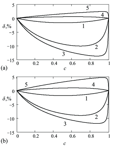
Figure 2: $\delta$ as a function of $c$ for mixtures of (a) prolate spheroids (aspect ratio 2) and (b) oblate spheroids (aspect ratio 0.5) embedded in a uniform isotropic host. The permittivities $\varepsilon_{0}$ and $\varepsilon$ are: 2 and 10 (curve 1); 2 and 100 (2); 2 and 1000 (3); 10 and 2 (4); 1000 and 2 (5).

Several facts are clearly seen for these systems. (1) In the limiting case of diluted mixtures, $\delta\rightarrow 0$. (2) Even if the contrast $\kappa\equiv\varepsilon/\varepsilon_{0}$ is extremely high, $|\delta|$ does not exceed $3\div 4\%$ for $c<0.5c_{\rm max}$ and $5\div 7\%$ for $c\in(0.5c_{\rm max},c_{\rm max})$. (3) For moderate values of $c$, $|\delta|$ increases when either $c$, or $\kappa$, or they both increase; depending on $\kappa$, $|\delta|$ can be as high as $10\div 15\%$. (4) Compared to Eq. (III.1), Eq. (26) predicts a smaller magnitude for the ellipsoidal-shape influence on the formation of $\varepsilon_{\rm eff}$: for a given $c$, $|\varepsilon_{\rm eff}^{(\ref{eq:eq28a})}-\varepsilon_{0}|<|\varepsilon_{\rm eff}^{(\ref{eq:eq24a})}-\varepsilon_{0}|$. The physical explanation for these tendencies is, in our opinion, as follows: multiple mutual polarizations and short-range correlations between ellipsoidal particles effectively reduce the anisotropy effects induced by a single particle. Unfortunately, the lack of numerical data for the systems under consideration does not allow us to check directly which of Eqs. (26) and (III.1) does better.

IV BRUGGEMAN-TYPE MIXING FORMULAS

As the concentration of anisotropic particles in a mixture becomes greater than $c_{\rm max}$, two kinds of phenomena can be expected. On one hand, strong mutual influences can trigger various physicochemical processes, affecting the textures and dielectric properties of the particles and host medium. On the other hand, interparticle contacts can cause the formation of coarse aggregates of particles; as a result, asymmetry between the disperse phase and the host medium fades away. In the limit, the original mixture, including particles of $s$ sorts, can be viewed as a system of $s+1$ components, filling chaotically located regions with irregular complex boundaries.

It was already mentioned that for concentrated mixtures, the Bruggeman mixing rule is often believed to be superior to the MG-type mixing rules. However, the accuracy and range of validity of this rule have remained disputable (for relevant details, see extensive review bib:Brosseau2006 ). To a great extent, the situation is explained by the lack of accurate electromagnetic solutions for disordered systems; as a result, most arguments for the Bruggeman rule are based on a dipolar approximation, valid for low concentrations of particles. The purpose of this section is to shed some light on theses issues. Namely, we show that the Bruggeman-type formulas are obtainable within the proposed compact-group approach under appropriate assumptions. In addition, system-dependent deviations from the classical mixing rules are expected to occur, provided physical and chemical processes change the dielectric and structural parameters of the mixture constituents.

To begin with, we remind that Eq. (13) and (14) are valid for any mixture satisfying the conditions of macroscopical homogeneity and isotropy. They form the basis for analysis of particular structural models of mixtures, which are formulated in terms of the local permittivity tensor $\varepsilon_{ik}({\rm{\bf r}})$. For instance, the above MG-type mixing rules (see Section III) are based on the model expression (1). Now, let us suppose that all components of a mixture, including the host medium, can be treated symmetrically in the following sense: there exists a fictitious (effective) medium, of permittivity $\epsilon$, such that the real mixture is macroscopically equivalent, in its dielectric properties, to a macroscopically homogeneous and isotropic system of nonoverlapping regions occupied by the components of the real mixture and embedded into this fictitious medium (see Fig. 3).

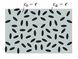
Figure 3: Effective medium approximation for the mixture shown in Fig. 1.

If combining the components into a real mixture does not change their properties, then the deviations of the local permittivity in the system from the value $\epsilon$ can be written as $\Delta\widetilde{\varepsilon}_{ik}({\rm{\bf r}},\Omega_{\lambda_{a}})=\varepsilon_{ik}({\rm{\bf r}},\Omega_{\lambda_{a}})-\epsilon\delta_{ik}$ for regions $\Omega_{\lambda_{a}}$, occupied by particles of sort $a$, and as $(\varepsilon_{0}-\epsilon)\delta_{ik}$ for the rest of space, occupied by the host. Correspondingly, the local permittivity deviations $\delta\varepsilon_{ik}({\rm{\bf r}})$ from $\epsilon$ due to a compact group, of the above regions, present at the point $\bf{r}$ in the system can be modelled as

$$\delta\varepsilon_{ik}({\rm{\bf r}})=(\varepsilon_{0}-\epsilon)\delta_{ik}\,\Pi({\rm{\bf r}})+{\sum\limits_{a=1}^{s}{\sum\limits_{\lambda_{a}=1}^{N_{a}}{\Delta\widetilde{\varepsilon}_{ik}({\rm{\bf r}},{\rm\Omega}_{\lambda_{a}})\,\Pi({\rm{\bf r}},{\rm\Omega}_{\lambda_{a}})}}},$$ (35)

where

$$\Pi({\rm{\bf r}})=1-{\sum\limits_{a=1}^{s}{\sum\limits_{\lambda_{a}=1}^{N_{a}}\Pi({\rm{\bf r}},{\rm\Omega}_{\lambda_{a}})}}$$

is the characteristic function for the space occupied by the host of the real mixture. Carrying out manipulations similar to those in Section III and introducing the total volume concentration $c=\sum_{a=1}^{s}c_{a}$ of the disperse particles, we find:

$${\frac{{\varepsilon_{\rm eff}}-{\epsilon}}{2{\epsilon}+{\varepsilon_{\rm eff}}}}=(1-c){\frac{{\varepsilon_{0}}-{\epsilon}}{2{\epsilon}+{\varepsilon_{0}}}}+{\frac{{4\pi}}{{3}}}{\sum\limits_{a=1}^{s}}{n_{a}}\widetilde{\alpha}_{\rm eff}^{a},$$ (36)

$$\widetilde{\alpha}_{\rm eff}^{a}={\frac{{1}}{{3}}}\left({\widetilde{\alpha}_{11}^{a}+\widetilde{\alpha}_{22}^{a}+\widetilde{\alpha}_{33}^{a}}\right),$$ (37)

$$\widetilde{\alpha}_{ii}^{a}={\frac{{3}}{{4\pi}}}{\int\limits_{v_{a}}{d{\rm{\bf r}}}}{\frac{{\varepsilon_{ii}^{a}({\rm{\bf r}})-\epsilon}}{{2\epsilon+\varepsilon_{ii}^{a}({\rm{\bf r}})}}},\quad i=1,\,2,\,3.$$ (38)

The quantities $\widetilde{\alpha}_{\rm eff}^{a}$ can be interpreted as the effective polarizabilities of particles of sort $a$ in the fictitious effective medium of permittivity $\epsilon$. For mixtures of particles filled with homogeneous anisotropic or homogeneous isotropic dielectrics, we respectively have:

$$\ {\frac{{\varepsilon_{\rm eff}}-{\epsilon}}{2{\epsilon}+{\varepsilon_{\rm eff}}}}=(1-c){\frac{{\varepsilon_{0}}-\epsilon}{2\epsilon+\varepsilon_{0}}}+{\frac{{1}}{{3}}}{\sum\limits_{a=1}^{s}{c_{a}{\sum\limits_{i=1}^{3}{{\frac{{\varepsilon_{ii}^{a}-\epsilon}}{{2\epsilon+\varepsilon_{ii}^{a}}}}}}}},$$ (39)

$${\frac{{\varepsilon_{\rm eff}}-{\epsilon}}{2{\epsilon}+{\varepsilon_{\rm eff}}}}=(1-c){\frac{{\varepsilon_{0}}-\epsilon}{2\epsilon+\varepsilon_{0}}}+{\sum\limits_{a=1}^{s}{c_{a}{{\frac{{\varepsilon^{a}-\epsilon}}{{2\epsilon+\varepsilon^{a}}}}}}}.$$ (40)

In the above formulas, the permittivity $\epsilon$ is unknown and should be considered as an adjustable parameter. Under the additional assumption that the fictitious effective medium is macroscopically equivalent, in its dielectric properties, to the mixture itself, $\epsilon=\varepsilon_{\rm eff}$, the left-hand sides in Eqs. (36), (39), and (40) vanish, and we arrive at generalizations of the classical Bruggeman fixing rule. Note also that particular forms of Eq. (40) are known in the literature (see, for instance, Ref. bib:Musal1988, , where it was obtained within a dipolar analysis for the case of identical spherical inclusions). Finally, for $\epsilon=\varepsilon_{0}$, the results of Section III are obtained.

For sufficiently concentrated mixtures, large aggregates of particles can themselves be treated as structural units, with scalar (on the average) permittivities. Modelling such a mixture as a system of nonoverlapping regions occupied by substances (the host medium of the real mixture among them) with different permittivities and embedded into a fictitious medium of permittivity $\epsilon$ (see Fig. 4),

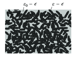
Figure 4: Modelling the mixture shown in Fig. 1 for the case of high particle concentrations.

we again arrive at Eqs. (36)–(38), with $\varepsilon_{ii}^{a}({\rm\bf r})=\varepsilon^{a}({\rm\bf r})$, and Eq. (40), with $\varepsilon^{a}({\rm\bf r})=\varepsilon^{a}={\rm const}$. Now, $\varepsilon^{a}({\rm\bf r})$ stands for the averaged-permittivity distribution within the region of sort $a$, $n_{a}$ is the concentration of such regions, $v_{a}$ indicates integration over the region of sort $a$, and $c_{a}$ stands for the volume concentration of the substance of sort $a$.

V CONCLUSION

The main results and conclusions of this paper are as follows.

(1) The compact-group method for study of effective dielectric properties of finely dispersed mixtures is generalized to the case where the mixtures are composed of anisotropic inhomogeneous particle. Based on this generalization, new mixing rules for mixtures of hard dielectric particles are derived and their ranges of validity are discussed; in appropriate cases, the rules obtained agree with the classical Maxwell-Garnet and Bruggeman rules. It should be emphasized that within our method, the contributions from multiple polarization and short-range correlation effects of all orders are effectively taken into account.

(2) That fact that mixing rules of both types are obtainable (under appropriate approximations) within a single formalism is taken by us as strong evidence of the validity of basic relations (13) and (14). If this is really the case, much emphasis in further effective permittivity studies should be put on modelling, in terms of the permittivity distribution, of the structure and dielectric properties of the constituents of a real mixture. Deviations of these properties from those of isolated constituents should manifest themselves as deviations from the classical mixing rules and their modifications obtained in the present work.

(3) The averages in Eqs. (13) and (14) are in fact statistical, according to the analysis in Section II. Consequently, Eqs. (13) and (14) can be used to develop a statistical theory of effective permittivity. In particular, proceeding in this way and using the general properties of particle distribution functions for macroscopically homogeneous and isotropic systems of balls, one can infer that it is the hardness of the balls that lies at the heart of the classical MG mixing rule.

- (1) J. C. Maxwell-Garnett, Phil. Trans. R. Soc. London, Ser. A 203, 385 (1904).
- (2) C. Brosseau, J. Phys. D: Appl. Phys. 39, 1277 (2006).
- (3) C. F. Bohren and D. R. Huffman, Absorption and Scattering of Light by Small Particles (Wiley, New York, 1983).
- (4) A. Sihvola, Electromagnetic Mixing Formulas and Applications. IEE Electromagnetic Waves Series, Vol. 47 (IEE, London, 1999).
- (5) L. Tsang and J. A. Kong, Scattering of Electromagnetic Waves: Advanced Topics (Wiley, New York, 2001).
- (6) F. Claro and R. Rojas, Phys. Rev. B 43, 6369 (1991).
- (7) L. Fu, P. B. Macedo, and L. Resca, Phys. Rev. B 47, 13818 (1993).
- (8) B. Abeles and J. I. Gittleman, Appl. Opt. 15, 2328 (1976).
- (9) A. Spanoudaki and R. Pelster, Phys. Rev. B 64, 064205 (2001).
- (10) F. Wu and K. W. Whites, IEEE Trans. Antennas Propag. 49, 1174 (2001).
- (11) D. A. Robinson and S. P. Friedman, J. Non-Cryst. Solids 305, 261 (2002).
- (12) P. Mallet, C. A. Guérin, and A. Sentenac, Phys. Rev. B 72, 014205 (2005).
- (13) D. A. G. Bruggeman, Ann. Phys. Leipzig 24, 636 (1935).
- (14) O. Levy and D. Stroud, Phys. Rev. B 56, 8035 (1997).
- (15) L. Jylhä and A. Sihvola, J. Phys. D: Appl. Phys. 40, 4966 (2007).
- (16) M. Lax, Phys. Rev. 85, 621 (1952).
- (17) W. Lamb, D. M. Wood, and N. W. Ashcroft, Phys. Rev. B 21, 2248 (1980).
- (18) L. Tsang and J. A. Kong, J. Appl. Phys. 51, 3465 (1980).
- (19) V. A. Davis and L. Schwartz, Phys. Rev. B 31, 5155 (1985).
- (20) V. L. Kuz’min, Zh. Eksp. Teor. Fiz. 127, 1173 (2005) [JETP 100, 1035, (2005)].
- (21) M. Ya. Sushko, Zh. Eksp. Teor. Fiz. 132, 478 (2007) [JETP 105, 426 (2007)].
- (22) L. D. Landau and E. M. Lifshitz, Course of Theoretical Physics, Vol. 8: Electrodynamics of Continuos Media, 2nd ed. (Nauka, Moscow, 1982; Pergamon, Oxford, 1984).
- (23) M. Ya. Sushko and S. K. Kris’kiv, Zh. Tekhn. Fiz. 79, 97 (2009) [Techn. Phys. 54, 423 (2009)].
- (24) V. B. Beresteckii, E. M. Lifshitz, and L. P. Pitaevskii, Course of Theoretical Physics, Vol. 4: Quantum Electrodynamics, 2nd ed. (Nauka, Moscow, 1980; Pergamon, Oxford, 1982).
- (25) M. Ya. Sushko, Zh. Eksp. Teor. Fiz. 126, 1355 (2004) [JETP 99, 1183 (2004)].
- (26) H. M. Musal, H. T. Hahn, and Bush G. G., J. Appl. Phys. 63, 3768 (1988).