MC@NLO for the hadronic decay of Higgs bosons in associated production with vector bosons

Abstract:

In this article we describe simulations of the hadronic decay of Higgs bosons produced in association with vector bosons at linear and hadronic colliders. We use the Monte Carlo at next-to-leading-order (MC@NLO) matching prescription with the Herwig++ event generator to predict various spectra of the resulting $b\bar{b}$ pairs and compare our results with leading order and matrix element correction predictions.

1 Introduction

The Higgs boson is an elusive particle which couples to particles according to their mass and so is weakly coupled to quarks and leptons. The dominant production mechanisms of Higgs bosons at hadron colliders is from gluon-gluon fusion and vector boson fusion. In this paper, we consider another mechanism which may be more relevant to an experimental search. This is the associated production of Higgs bosons with vector bosons. This production mechanism, $p\bar{p}\rightarrow WH/ZH+X$, is the most promising discovery channel for a light Standard Model (SM) Higgs boson at the Tevatron. This is because the Higgs, which decays predominantly into $b\bar{b}$ pairs, can be tagged by the associated vector boson.

Such processes can be simulated in parton shower generators which resum soft and collinear leading logarithmic, as well as an important subset of next-to-leading logarithmic contributions to all orders. These simulations can further be improved by matching the parton shower to higher order matrix elements. One way in which this is done in the generic parton shower generators is through the use of the matrix element correction [1] which generates harder emissions in regions outside the reach of the parton shower at a rate given by the matrix element. A more rigorous matching procedure is the MC@NLO method [2, 3, 4, 5, 6] which has been implemented for a multitude of processes in the HERWIG event generator [7] and for some processes [8] in its successor the Herwig++ event generator [9, 10]. More recently, another matching method was proposed, called the POsitive Weighted Hardest Emission Generator (POWHEG) [11, 12], which achieves the same aim as MC@NLO, with the creation of positive weighted events and is furthermore independent of the shower generator used. The POWHEG method has been applied to $Z$ pair hadroproduction [13], heavy flavour production [14], $e^{+}e^{-}$ annihilation to hadrons [15], Drell-Yan vector boson production [16, 17] and top pair production at the ILC [18].

In this paper, we aim to simulate the NLO hadronic decay of the light Higgs boson produced in association with a vector boson using the MC@NLO method. The parton shower generator we will be employing is Herwig++. In Section 2, we first discuss the cross-sections for associated production of the Higgs boson with a vector boson and its subsequent hadronic decay rate. We then discuss the application of the MC@NLO method to the decay in Section 3. In Section 4, we show some comparative distributions obtained from the parton shower and in Section 5 we summarize our conclusions. Finally, it should be noted that in this paper, we do not apply the MC@NLO method to the initial state emissions.

2 Cross-sections and decay rates

2.1 Associated Higgs production with a $W$ boson from $q\bar{q}$ annihilation

The process $q(p_{q})+\bar{q}^{\prime}(p_{\bar{q}}^{\prime})\rightarrow W^{*}\rightarrow W(p_{W})+H(p_{H})$ is illustrated in Figure 1.

Figure 1: Associated $WH$ boson production.

If we define the center of mass energy squared of the partonic system by

$$s = (p_{q}+p_{\bar{q}^{\prime}})^{2}\,,$$ (1)

we have for the differential cross-section [19],

$$\frac{d\sigma_{p}}{d\cos\theta^{*}} = \frac{G_{F}^{2}M_{W}^{2}V_{q\bar{q}^{\prime}}^{2}}{\cos^{2}\theta_{W}}\frac{\beta_{W}\gamma_{W}M_{W}^{3}}{48\pi s^{3/2}}\left(\frac{s+M_{W}^{2}-M_{H}^{2}}{s-M_{W}^{2}}\right)^{2}[2(1-\beta_{W}^{2})+\beta_{W}^{2}\sin^{2}\theta^{*}]\,,$$ (2)

where $\theta^{*}$ is the angle between the $W$ boson and the quark in the partonic CMF, $G_{F}$ is the Fermi coupling constant, $\theta_{W}$ is the Weinberg mixing angle, $M_{W}$ and $M_{H}$ are respectively the $W$ and Higgs boson masses and $V_{q\bar{q}^{\prime}}$ is the relevant CKM matrix element. $\beta_{W}$ is the speed of the $W$ boson in the partonic CMF and is given by

$$\beta_{W}=\frac{\sqrt{[s-(M_{W}+M_{H})^{2}][s-(M_{W}-M_{H})^{2}]}}{s-M_{H}^{2}+M_{W}^{2}}\;.$$ (3)

The relativistic boost factor $\gamma_{W}$ is $(1-\beta_{W}^{2})^{-1/2}$. Equation 2 when integrated gives for the total partonic cross-section,

$$\sigma_{p} = \frac{G_{F}^{2}M_{W}^{2}V_{q\bar{q}^{\prime}}^{2}}{\cos^{2}\theta_{W}}\frac{\beta_{W}\gamma_{W}M_{W}^{3}}{12\pi s^{3/2}}\left(\frac{s+M_{W}^{2}-M_{H}^{2}}{s-M_{W}^{2}}\right)^{2}\left[1-\frac{2\beta_{W}^{2}}{3}\right]\;.$$ (4)

Convolving this with parton distribution functions (PDFs), we obtain the hadronic cross-section as

$$\sigma_{h}=\int_{\tau}^{1}dx_{1}\int_{\tau/x_{1}}^{1}dx_{2}[f_{q}(x_{1},M_{W}^{2})f_{\bar{q}^{\prime}}(x_{2},M_{W}^{2})+x_{1}\leftrightarrow x_{2}]\sigma_{p}\,,$$ (5)

where $x_{1},x_{2}$ are the momentum fractions of the incoming partons and taking $S$ as the hadronic beam-beam center-of-mass energy, we have $s=x_{1}x_{2}S$.

2.2 Associated Higgs production with a $Z$ boson from $e^{+}e^{-}$ annihilation

The differential cross-section for the process $e^{+}e^{-}\rightarrow Z^{*}\rightarrow ZH$

Figure 2: Associated $ZH$ production.

is given by [20]

$$\frac{d\sigma}{d\cos\theta^{*}} = \frac{G_{F}^{2}M_{W}^{2}}{\cos^{2}\theta_{W}}\frac{\beta_{Z}\gamma_{Z}M_{Z}^{3}}{32\pi s^{3/2}}\left(\frac{s+M_{Z}^{2}-M_{H}^{2}}{s-M_{Z}^{2}}\right)^{2}\times$$ (6)

$$\left[1-4\sin^{2}\theta_{W}+8\sin^{4}\theta_{W}\right][2(1-\beta_{Z}^{2})+\beta_{Z}^{2}\sin^{2}\theta^{*}]\,,$$

where $\theta^{*}$ is the angle between the electron and the $Z$ boson in the CMF, $s$ is the center-of-mass energy and $\gamma_{Z}$ and $\beta_{Z}$ are obtained from the analogous expressions for $W$ production in section 2.1 by substituting $M_{Z}$ for $M_{W}$. Equation 6 integrated over $\cos\theta^{*}$ gives

$$\sigma(e^{+}e^{-}\rightarrow ZH) = \frac{G_{F}^{2}M_{W}^{2}}{\cos^{2}\theta_{W}}\frac{\beta_{Z}\gamma_{Z}M_{Z}^{3}}{8\pi s^{3/2}}\left(\frac{s+M_{Z}^{2}-M_{H}^{2}}{s-M_{Z}^{2}}\right)^{2}\times$$ (7)

$$\left[1-4\sin^{2}\theta_{W}+8\sin^{4}\theta_{W}\right]\left[1-\frac{2}{3}\beta_{Z}^{2}\right]\;.$$

2.3 Higgs boson decay to $b\bar{b}$ pairs

2.3.1 Lowest Order decay rate

Figure 3: Lowest order Higgs hadronic decay rate.

The lowest-order decay rate for this process, illustrated in Figure 3, is given by

$$\Gamma_{B}(H\rightarrow b\bar{b})=\frac{3G_{F}m_{b}^{2}}{4\sqrt{2}\pi}M_{H}\beta_{0}^{3}\,,$$ (8)

where $m_{b}$ is the mass of the bottom quark and $\beta_{0}=\sqrt{1-\frac{4m_{b}^{2}}{M_{H}^{2}}}$.

2.3.2 Virtual radiative corrections

Figure 4: Virtual corrections (a): vertex correction (b),(c): self-energy corrections.

If one uses the on-shell renormalization scheme, the self-energy diagrams in Figures 4(b) and 4(c) are cancelled by counter-term diagrams leaving us with the vertex correction in Figure 4(a) and its counter-term. When evaluated in the massive gluon regularization scheme, the final result is [21],

$$\Gamma_{V} = \frac{\alpha_{S}C_{F}}{\pi}\Gamma_{B}\left[-\left(\frac{1+\beta_{0}^{2}}{2\beta_{0}}\ln\frac{1+\beta_{0}}{1-\beta_{0}}\right)\ln\frac{m_{b}^{2}}{\mu^{2}}\right.$$ (9)

$$+ \left.\frac{1+\beta_{0}^{2}}{\beta_{0}}\left\{{\rm Li}_{2}\left(\frac{1-\beta_{0}}{1+\beta_{0}}\right)+\ln\frac{1+\beta_{0}}{2\beta_{0}}\ln\frac{1+\beta_{0}}{1-\beta_{0}}-\frac{1}{4}\ln^{2}\frac{1+\beta_{0}}{1-\beta_{0}}+\frac{\pi^{2}}{3}\right\}\right.$$

$$+ \left.\frac{1-\beta_{0}^{2}}{\beta_{0}}\ln\frac{1+\beta_{0}}{1-\beta_{0}}-1\right]\,,$$

where we have introduced the gluon mass $\mu$ to regulate the infrared singularity in Figure 4(a).

2.3.3 Real emission corrections

Figure 5: Real gluon emission.

Using the following relations for the energy fractions of the $b$ and $\bar{b}$ quarks in terms of the parton momenta in the Higgs rest frame,

$$x_{b} = 1-\frac{2p_{\bar{b}}\cdot k}{M_{H}^{2}}\,,$$

$$x_{\bar{b}} = 1-\frac{2p_{b}\cdot k}{M_{H}^{2}}\,,$$ (10)

we have for the real emission decay rate, the following expression:

$$\frac{d\Gamma_{R}}{dx_{b}dx_{\bar{b}}} = \Gamma_{B}\frac{\alpha_{S}C_{F}}{2\pi}\mathcal{M}$$ (11)

$$= \Gamma_{B}\frac{\alpha_{S}C_{F}}{2\pi\beta_{0}^{3}}\left[\frac{(1-x_{b})^{2}+(1-x_{\bar{b}})^{2}+2(1-2\rho)(x_{b}+x_{\bar{b}}-1-4\rho)}{(1-x_{b})(1-x_{\bar{b}})}\right.$$

$$+ \left.4\rho\left\{\frac{1}{1-x_{b}}+\frac{1}{1-x_{\bar{b}}}\right\}-2\rho(1-4\rho)\left\{\frac{1}{(1-x_{b})^{2}}+\frac{1}{(1-x_{\bar{b}})^{2}}\right\}+2\right]\,,$$

where $\rho=\frac{m_{b}^{2}}{M_{H}^{2}}$. This can be integrated in the massive gluon scheme to get,

$$\Gamma_{R} = \Gamma_{B}\frac{\alpha_{S}C_{F}}{2\pi}\left[\left(\frac{1+\beta_{0}^{2}}{2\beta_{0}}\ln\frac{1+\beta_{0}}{1-\beta_{0}}\right)\ln\frac{m_{b}^{2}}{\mu^{2}}\right.$$ (12)

$$+ \left.\frac{1+\beta_{0}^{2}}{2\beta_{0}}\left\{3{\rm Li}_{2}\left(\frac{1-\beta_{0}}{1+\beta_{0}}\right)+2{\rm Li}_{2}\left(-\frac{1-\beta_{0}}{1+\beta_{0}}\right)-\ln\frac{2}{1+\beta_{0}}\ln\frac{1+\beta_{0}}{1-\beta_{0}}\right.\right.$$

$$+ \left.\left.\frac{1}{4}\ln^{2}\frac{1+\beta_{0}}{1-\beta_{0}}+\ln\frac{1+\beta_{0}}{2\beta_{0}}\ln\frac{1+\beta_{0}}{1-\beta_{0}}-\frac{\pi^{2}}{3}\right\}-3\ln\frac{4}{1-\beta_{0}^{2}}-4\ln\beta_{0}\right.$$

$$+ \left.\frac{1}{16\beta_{0}^{3}}\left\{3+2\beta_{0}^{2}+3\beta_{0}^{4}\right\}\ln\frac{1+\beta_{0}}{1-\beta_{0}}+\frac{1}{8\beta_{0}^{2}}\{-3+29\beta_{0}^{2}\}\right]\;.$$

Summing this with $\Gamma_{B}$ and $\Gamma_{V}$ in equation 9, the dependence of the gluon mass $\mu$ disappears to give,

$$\Gamma_{\rm NLO}=\Gamma_{B}\left[1+\frac{\alpha_{S}C_{F}}{\pi}\Pi\right]\,,$$ (13)

where

$$\Pi = \frac{1}{\beta_{0}}\left[(1+\beta_{0}^{2})\left\{4{\rm Li}_{2}\left(\frac{1-\beta_{0}}{1+\beta_{0}}\right)+2{\rm Li}_{2}\left(-\frac{1-\beta_{0}}{1+\beta_{0}}\right)-3\ln\frac{2}{1+\beta_{0}}\ln\frac{1+\beta_{0}}{1-\beta_{0}}\right.\right.$$ (14)

$$- \left.\left.2\ln\beta_{0}\ln\frac{1+\beta_{0}}{1-\beta_{0}}\right\}-3\beta_{0}\ln\frac{4}{1-\beta_{0}^{2}}-4\beta_{0}\ln\beta_{0}\right]$$

$$+ \frac{1}{16\beta_{0}^{3}}[3+34\beta_{0}^{2}-13\beta_{0}^{4}]\ln\frac{1+\beta_{0}}{1-\beta_{0}}+\frac{3}{8\beta_{0}^{2}}[-1+7\beta_{0}^{2}]\;.$$

Also from equations 9, 11 and 12, we note that $\Gamma_{V}$ can be written in terms of the real emission matrix element squared $\mathcal{M}$ as

$$\Gamma_{V} = \Gamma_{B}\frac{\alpha_{S}C_{F}}{2\pi}\left[\left\{-\int dx_{b}dx_{\bar{b}}\hskip 7.22743pt\mathcal{M}\right\}+2\Pi_{V}\right]\,,$$ (15)

where

$$\Pi_{V} = \frac{1-\beta_{0}^{2}}{\beta_{0}}\ln\frac{1+\beta_{0}}{1-\beta_{0}}+\frac{1+\beta_{0}^{2}}{\beta_{0}}\left\{4{\rm Li}_{2}\left(\frac{1-\beta_{0}}{1+\beta_{0}}\right)+2{\rm Li}_{2}\left(-\frac{1-\beta_{0}}{1+\beta_{0}}\right)\right.$$ (16)

$$+ \left.2\ln\frac{1+\beta_{0}}{2\beta_{0}}\ln\frac{1+\beta_{0}}{1-\beta_{0}}-\ln\frac{2}{1+\beta_{0}}\ln\frac{1+\beta_{0}}{1-\beta_{0}}\right\}-3\ln\frac{4}{1-\beta_{0}^{2}}-4\ln\beta_{0}$$

$$+ \frac{1}{16\beta_{0}^{3}}\{3+18\beta_{0}^{2}+3\beta_{0}^{4}\}\ln\frac{1+\beta_{0}}{1-\beta_{0}}+\frac{3}{8\beta_{0}^{2}}\{-1+7\beta_{0}^{2}\}\;.$$

3 MC@NLO method

The phase space for gluon emission is given in terms of the Dalitz plot variables $x_{b},x_{\bar{b}}$ by

$$\lambda(x_{b}^{2}-\rho,x_{\bar{b}}^{2}-\rho,(2-x_{b}-x_{\bar{b}})^{2})\leq 0\,,$$ (17)

where the function $\lambda$ is defined by,

$$\lambda(x,y,z)=x^{2}+y^{2}+z^{2}-2xy-2yz-2xz\;.$$ (18)

This is equivalent to the condition

$$(1-x_{b})(1-x_{\bar{b}})(x_{b}+x_{\bar{b}}-1)>\rho(2-x_{b}-x_{\bar{b}})^{2}\,,$$ (19)

Figure 6 shows the corresponding phase space region

Figure 6: Phase space for gluon emission.

where we have labeled as ${\bf P}$ the emission region and ${\bf O}$ the region outside the ${\bf P}$ but in the half-triangle $(1-x_{b})(1-x_{\bar{b}})(x_{b}+x_{\bar{b}}-1)>0$.

Now using equation 11 and 15, we can re-write $\Gamma_{\rm NLO}$ in integral form as,

$$\Gamma_{\rm NLO}=\sigma_{B}\int_{\bf P}dx_{b}dx_{\bar{b}}\left[2-\frac{\alpha_{S}C_{F}}{2\pi}\{\mathcal{M}-4\Pi_{V}\}+\frac{\alpha_{S}C_{F}}{2\pi}\mathcal{M}\right]+\Gamma_{B}\int_{\bf O}dx_{b}dx_{\bar{b}}\left[2+\frac{\alpha_{S}C_{F}}{2\pi}4\Pi_{V}\right]\;.$$ (20)

Now, if we define a functional $\mathcal{F}_{i}$ which represents hadronic final states generated by a parton shower starting from a configuration $i$, we can write down an overall generating functional for hadrons from Higgs boson decay as

$$\mathcal{F} = \Gamma_{B}\int_{\bf P}dx_{b}dx_{\bar{b}}\left[\mathcal{F}_{b\bar{b}}\left\{2-\frac{\alpha_{S}C_{F}}{2\pi}(\mathcal{M}-4\Pi_{V})\right\}+\mathcal{F}_{b\bar{b}g}\frac{\alpha_{S}C_{F}}{2\pi}\mathcal{M}\right]$$ (21)

$$+ \Gamma_{B}\int_{\bf O}dx_{b}dx_{\bar{b}}\mathcal{F}_{b\bar{b}}\left[2+\frac{\alpha_{S}C_{F}}{2\pi}4\Pi_{V}\right]\,,$$

where $\mathcal{F}_{b\bar{b}}$ is the functional representing shower final states resulting from the process $H\rightarrow b\bar{b}$ and $\mathcal{F}_{b\bar{b}g}$ represents final states from $H\rightarrow b\bar{b}g$.

There are two problems with this functional as it is written above. The first is the highly inefficient sampling that will be required to generate starting $b\bar{b}$ and $b\bar{b}g$ configurations according to the $\mathcal{M}$ since it is divergent in the soft and collinear regions of phase space. The second problem arises because when interfaced with the parton shower, leading order configurations starting with $b\bar{b}$ would radiate quasi-collinear gluons with a distribution given by the parton shower approximation to $\mathcal{M}$ which we shall call $\mathcal{M}_{C}$. These are already included in the starting $b\bar{b}g$ configurations. Likewise, some of the $b\bar{b}g$ configurations would include $b\bar{b}$-like configurations if the gluon is quasi-collinear to either the quark or anti-quark. This problem is often referred to as double-counting.

Before we discuss how to solve these problems, let us investigate $\frac{\alpha_{S}C_{F}}{2\pi}\mathcal{M}_{C}$. In the parton shower generator Herwig++, this is the massive quasi-collinear splitting function for the emission of a gluon from a quark [22]:

$$\frac{\alpha_{S}C_{F}}{2\pi}\mathcal{M}_{C}d\tilde{q}^{2}dz=\frac{\alpha_{S}C_{F}}{2\pi}\frac{d\tilde{q}^{2}}{\tilde{q}^{2}}\frac{dz}{1-z}\left[1+z^{2}-\frac{2m_{b}^{2}}{z\tilde{q}^{2}}\right]\;.$$ (22)

Here $z$ and $\tilde{q}$ are Herwig++ evolution variables and are respectively the light-cone momentum fraction of the quark after the emission of the gluon and an angular variable related to the relative transverse momentum of the quark after the emission [23]. The splitting function in equation 22 for the $b$ quark can be re-written in terms of the Dalitz plot variables as

$$\frac{\alpha_{S}C_{F}}{2\pi}\mathcal{M}_{C}dx_{b}dx_{\bar{b}}=\frac{\alpha_{S}C_{F}}{2\pi}\frac{dx_{b}dx_{\bar{b}}}{(1-x_{\bar{b}})\sqrt{x_{\bar{b}}^{2}-4\rho}}\left[\frac{1+z^{2}}{1-z}-\frac{2\rho}{1-x_{\bar{b}}}\right]\,,$$ (23)

where if $r$ is defined as

$$r=\frac{1}{2}\left(1+\frac{\rho}{1+\rho-x_{\bar{b}}}\right)\,,$$ (24)

then $z$ is given by

$$z=r+\frac{x_{b}-(2-x_{\bar{b}})r}{\sqrt{x_{\bar{b}}^{2}-4\rho}}\;.$$ (25)

Note that $x_{b},x_{\bar{b}}$ are given in terms of $z$, $r$ and $\tilde{q}$ by

$$x_{b} = 1-z(1-z)\frac{\tilde{q}^{2}}{M_{H}^{2}}\,,$$

$$x_{\bar{b}} = (2-x_{b})r+(z-r)\sqrt{x_{b}^{2}-4\rho}\;.$$ (26)

For emission from $\bar{b}$ anti-quark interchange $x_{b}$ and $x_{\bar{b}}$ in the equations above.

In Herwig++, the quasi-collinear region of phase space covered by the parton shower is defined by imposing the condition,

$$\tilde{q}^{2}<\frac{M_{H}^{2}}{2}(1+\sqrt{1-4\rho})\;.$$ (27)

The corresponding regions are shown in Figure 7 labeled ${\bf J_{b}},{\bf J_{\bar{b}}}$ whilst the unpopulated dead region is labeled ${\bf D}$. Note that region ${\bf P}$ in Figure 6 corresponds to the union of regions ${\bf\ J_{b}}$, ${\bf J_{\bar{b}}}$ and ${\bf D}$.

Figure 7: Phase space showing hard ${\bf D}$ and soft/collinear ${\bf J_{b}},{\bf J_{\bar{b}}}$ gluon emission regions.

Now going back to the functional defined in equation 21, if in the region ${\bf J}={\bf J_{b}}\cup{\bf J_{\bar{b}}}$, we subtract the parton shower approximation $\mathcal{M}_{C}$ from the second term in equation 21 and add it to the first term we get

$$\mathcal{F} = \Gamma_{B}\int_{\bf J}dx_{b}dx_{\bar{b}}\left[\mathcal{F}_{b\bar{b}}\left\{2-\frac{\alpha_{S}C_{F}}{2\pi}(\mathcal{M}-\mathcal{M}_{C}-4\Pi_{V})\right\}+\mathcal{F}_{b\bar{b}g}\frac{\alpha_{S}C_{F}}{2\pi}\{\mathcal{M}-\mathcal{M}_{C}\}\right]$$ (28)

$$+ \Gamma_{B}\int_{\bf D}dx_{b}dx_{\bar{b}}\left[\mathcal{F}_{b\bar{b}}\left\{2-\frac{\alpha_{S}C_{F}}{2\pi}(\mathcal{M}-4\Pi_{V})\right\}+\mathcal{F}_{b\bar{b}g}\frac{\alpha_{S}C_{F}}{2\pi}\mathcal{M}\right]$$

$$+ \Gamma_{B}\int_{\bf O}dx_{b}dx_{\bar{b}}\mathcal{F}_{b\bar{b}}\left[2+\frac{\alpha_{S}C_{F}}{2\pi}4\Pi_{V}\right]\;.$$

This is the MC@NLO method which solves the problem of double-counting in the parton shower regions ${\bf J}$. It also solves the problem of the sampling inefficiency since $\mathcal{M}\rightarrow\mathcal{M}_{C}$ in the divergent regions and therefore $\mathcal{M}-\mathcal{M}_{C}$ tends to $0$ there. In Appendix A, we describe the algorithm used for the evaluation of the above integrals and the generation of events. We also discuss how we regularize some residual divergences by the use of mappings in Appendix B.

The procedure followed for event generation for associated Higgs production is outlined below.

1. For $p\bar{p}$ annihilation use equation 5 to distribute the Mandelstam variables $x_{1},x_{2}$ and the angle $\theta^{*}$ according to the differential cross-section. From these variables, reconstruct the $W$ and Higgs boson four-momenta. For $e^{+}e^{-}$ annihilation, use equation 6 to distribute the angle $\theta^{*}$ and reconstruct the $Z$ and Higgs boson four-momenta.

2. In the rest frame of the Higgs boson, generate the Dalitz plot variables $x_{b},x_{\bar{b}}$ and event weight as described in Appendix A. Reconstruct the four-momenta of the quark, anti-quark and gluon in this frame.

3. Boost the four-momenta back to the lab frame.

More details about the MC@NLO method can be found in [2].

4 Results

Following the prescription above, events for associated Higgs boson production of mass $114$ GeV and decaying into $b\bar{b}$ pairs with $m_{b}=5$ GeV, were generated and interfaced with Herwig++ 2.3.0 [10]. The following approximations were considered:

1. The Herwig++ parton shower interfaced to leading order events (LO),

2. the parton shower interfaced to leading order events which are supplemented by matrix element corrected events in the dead region (ME),

3. the parton shower interfaced to events generated by the MC@NLO method (MC@NLO).

The two processes considered were:

1. associated $WH$ production from $q\bar{q}^{\prime}$ annihilation at the Tevatron (1.96 TeV),

2. associated $ZH$ production from $e^{+}e^{-}$ annihilation at the ILC (0.5 TeV).

The following distributions were considered and shown in Figures 8 - 10 for $q\bar{q}^{\prime}$ annihilation and associated $W$ boson production and Figures 11 - 13 for $e^{+}e^{-}$ annihilation and associated $Z$ boson production. In the simulations, only the leptonic decays of vector bosons were considered.

1. The mass of the $b\bar{b}$ pair before hadronization,

2. the energy of the $b\bar{b}$ pair,

3. the transverse momentum of the $b\bar{b}$ pair with respect to the beam axis,

4. the transverse momentum of the $b\bar{b}$ pair with respect to the direction of the vector boson,

5. the longitudinal momentum of the $b\bar{b}$ pair with respect to the beam axis,

6. the rapidity of the $b\bar{b}$ pair.

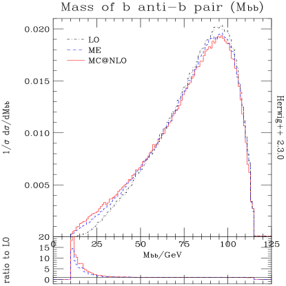
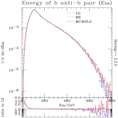
Figure 8: Mass and energy of the $b\bar{b}$ pair ($q\bar{q}^{\prime}$ annihilation).

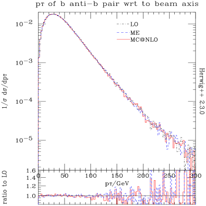
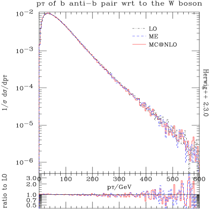
Figure 9: $p_{\rm T}$ of the $b\bar{b}$ pair w.r.t the beam axis and w.r.t the $W$ boson ($q\bar{q}^{\prime}$ annihilation).

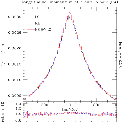
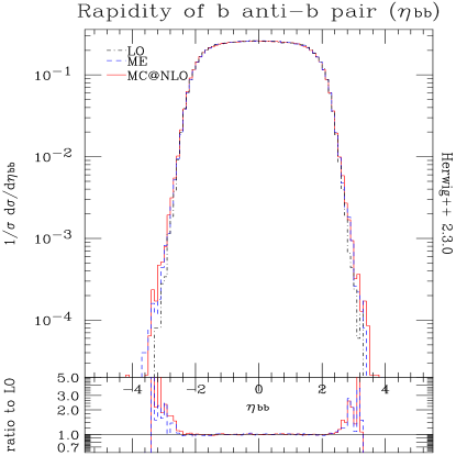
Figure 10: Longitudinal momentum and rapidity of the $b\bar{b}$ pair ($q\bar{q}^{\prime}$ annihilation).

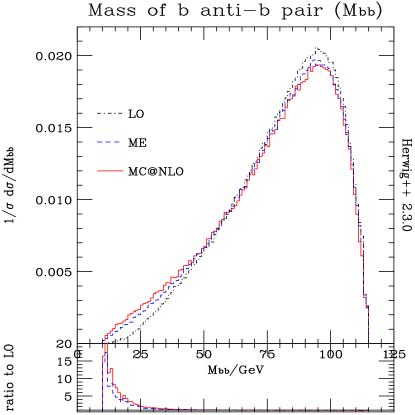
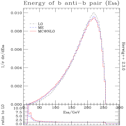
Figure 11: Mass and energy of the $b\bar{b}$ pair ($e^{+}e^{-}$ annihilation).

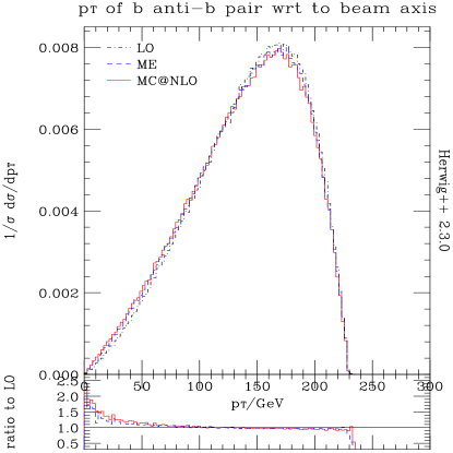
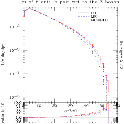
Figure 12: $p_{\rm T}$ of the $b\bar{b}$ pair w.r.t the beam axis and w.r.t the $Z$ boson ($e^{+}e^{-}$ annihilation).

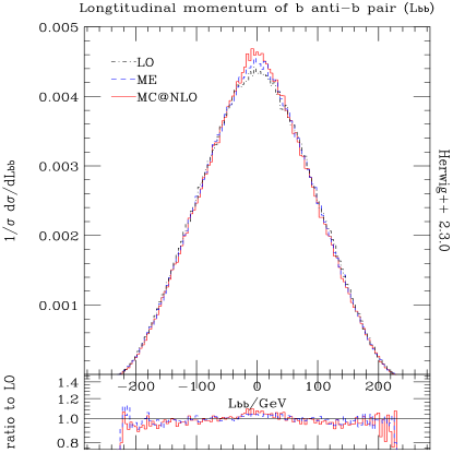
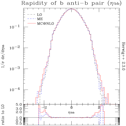
Figure 13: Longitudinal momentum and rapidity of the $b\bar{b}$ pair ($e^{+}e^{-}$ annihilation).

From the mass and energy reconstruction plots in Figures 8 and 11, we see that the extra gluon radiation simulated by the MC@NLO and matrix element correction methods smooth out the respective peaks due to the production of more low mass and energy $b\bar{b}$ pairs. We also observe as expected that the matrix element correction method underestimates the amount of hard gluon radiation when compared to the MC@NLO distributions.

For $q\bar{q}^{\prime}$ annihilation, the effect of this extra radiation on the transverse momenta plots is diminished by the initial state radiation from the incoming partons as can be seen in Figure 9. The effect is more clearly seen in the corresponding plots for $e^{+}e^{-}$ annihilation in Figure 12 where there is no initial state radiation. At leading order, the $b\bar{b}$ pairs are produced predominantly at right angles to the beam axis (equation 6), hence the peak at high $p_{\rm T}$ in the LO plot for $e^{+}e^{-}$ annihilation. The effect of extra gluon emission is to smooth out the peak as seen in the MC@NLO and ME correction plots. Likewise at leading order, the $b\bar{b}$ pairs are produced back-to-back with the associated $Z$ boson. The effect of gluon radiation is therefore to increase the transverse momentum of the $b\bar{b}$ with respect to the $Z$ boson. This is what is observed in the MC@NLO and ME correction distributions with the latter underestimating the amount of radiation in the tails in comparison with the former.

Finally, in Figures 10 and 13, the MC@NLO and ME correction method predict slightly more peaked distributions for the longitudinal momenta around the central value of $0$ GeV. This is a result of the loss of energy from the $b\bar{b}$ pairs due to extra gluon radiation. The rapidity distributions show the MC@NLO and ME correction methods predict the production of more high rapidity $b\bar{b}$ pairs in comparison to the leading order prediction. This arises as a result of more $b\bar{b}$ pairs being produced at low $p_{\rm T}$ with respect to the beam axis (Figure 12) and therefore higher absolute rapidity. It should also be noted that for both the longitudinal momenta and rapidity predictions, the ME correction method underestimates the amount of radiation in the tails of the distributions in comparison to the MC@NLO plots.

5 Conclusions

In this work we have realized the MC@NLO matching prescription for the decay of Higgs bosons produced in association with vector bosons at both the ILC and hadron colliders. This work was achieved within the framework of the Herwig++ Monte Carlo event generator.

We compared the MC@NLO predictions with those obtained via the matrix element correction method as well as leading order predictions. The effects of the hard radiation are visible in the reconstruction plots for the mass and energy of the $b\bar{b}$ pairs resulting from Higgs decay. Also visible is the effect on the longitudinal momenta and rapidity of the $b\bar{b}$ pairs.

Less visible is the effect on the $p_{\rm T}$ spectra for $q\bar{q}^{\prime}$ annihilation due to the dominant effects of initial state radiation. For $e^{+}e^{-}$ annihilation, the MC@NLO method predicts a softer spectrum for the $p_{\rm T}$ with respect to the beam axis and a harder spectrum with respect to the associated $Z$ boson.

The algorithm used for these processes will be publicly available with the forthcoming version of Herwig++. Although we have considered the associated production of Higgs and vector bosons in this paper, the MC@NLO algorithm can be interfaced with other Higgs boson production mechanisms, since here we only apply the method to the decay process.

6 Acknowledgements

We are grateful to the other members of the Herwig++ collaboration for developing the program that underlies the present work and for helpful comments. We are particularly grateful to Bryan Webber for constructive comments and discussions throughout. This work was supported by the UK Science and Technology Facilities Council, formerly the Particle Physics and Astronomy Research Council, and the European Union Marie Curie Research Training Network MCnet under contract MRTN-CT-2006-035606.

Appendix A Monte Carlo algorithm

The integrals in (28) can be evaluated using a variety of Monte Carlo methods. In this paper, the ‘Hit or Miss’ Monte Carlo method is used. This is the simplest and oldest form of Monte Carlo integration and essentially involves finding the area of a region in phase space by integrating over a larger region, a binary function which is $1$ in the region and $0$ elsewhere. The sampling method used for the points $x_{b},x_{\bar{b}}$ is the importance sampling method whereby more samples are taken from regions where the integrand is large and less from regions where it is small. This ensures that the sampled points have the same distribution as the integrand.

The following algorithm summarizes how the starting $b\bar{b}$ and $b\bar{b}g$ configurations were generated according to equation 28. In the discussion that follows, we work in the rest frame of a Higgs boson of mass $M_{H}=114$ GeV and $\alpha_{S}=\alpha_{S}(M_{H})=0.114$.

1. Randomly sample points $x_{b},x_{\bar{b}}$, in each of regions ${\bf J_{b}},{\bf J_{\bar{b}}}$, ${\bf D}$ and ${\bf O}$ of the phase space and using the ‘Hit Or Miss’ Monte Carlo method, evaluate the 5 integrals, $I_{J}^{(2)},I_{J}^{(3)},I_{D}^{(2)}$, $I_{D}^{(3)}$ and $I_{O}^{(2)}$ as well as their absolute sum, $I$.

   $$I_{J}^{(2)} = \int_{\bf J}dx_{b}dx_{\bar{b}}\left[2-\frac{\alpha_{S}}{2\pi}C_{F}\left\{\mathcal{M}-\mathcal{M}_{C}-\Pi_{V}\right\}\right]\,,$$

   $$I_{J}^{(3)} = \int_{\bf J}dx_{b}dx_{\bar{b}}\frac{\alpha_{S}}{2\pi}C_{F}[\mathcal{M}-\mathcal{M}_{C}]\,,$$

   $$I_{D}^{(2)} = \int_{\bf D}dx_{b}dx_{\bar{b}}\left[2-\frac{\alpha_{S}}{2\pi}C_{F}\left\{\mathcal{M}-\Pi_{V}\right\}\right]\,,$$

   $$I_{D}^{(3)} = \int_{\bf D}dx_{b}dx_{\bar{b}}\frac{\alpha_{S}}{2\pi}C_{F}\mathcal{M}\,,$$

   $$I_{O}^{(2)} = \int_{\bf O}dx_{b}dx_{\bar{b}}\left[2+\frac{\alpha_{S}}{2\pi}C_{F}\Pi_{V}\right]\,,$$

   $$I = \mid{I_{J}^{(2)}}\mid+\mid{I_{J}^{(3)}}\mid+\mid{I_{D}^{(2)}}\mid+\mid{I_{D}^{(3)}}\mid+\mid{I_{O}^{(2)}}\mid\;.$$ (29)

   Note also the maximum values of the integrands in $I_{J}^{(3)}$ and $I_{D}^{(3)}$.

2. The eventual proportion of $b\bar{b}$ Monte Carlo events will be determined by the ratio $\frac{\mid{I_{J}^{(2)}}\mid+\mid{I_{D}^{(2)}}\mid+\mid{I_{O}^{(2)}}\mid}{I}$. Likewise, the proportion of $b\bar{b}g$ events in the soft regions ${\bf J_{b}},{\bf J_{\bar{b}}}$ and the hard region ${\bf D}$ are determined by the ratios $\frac{\mid{I_{J}^{(3)}}\mid}{I}$ and $\frac{\mid{I_{D}^{(3)}}\mid}{I}$ respectively. The algorithm below is then used to importance-sample the $b\bar{b}g$ events so that the corresponding ($x_{b},x_{\bar{b}}$) values of the Monte Carlo events have the same distribution as the integrands in $I_{J}^{(3)}$ and$I_{D}^{(3)}$:

   1. For event generation in region ${\bf L}$ (where ${\bf L}$ is one of ${\bf D},{\bf J_{b}}$ or ${\bf J_{\bar{b}}}$), randomly select a point $x_{b},x_{\bar{b}}$ in that region.
      

   2. Evaluate the absolute value of the integrand in $I_{L}^{(3)}$ for this point, $\mid{w(x_{b},x_{\bar{b}})}\mid$.
      Is $\mid{w(x_{b},x_{\bar{b}})}\mid$ $>R$ $\mid{w_{\rm max}}\mid$ ? ($R$ is a random number between 0 and 1 and $\mid{w_{\rm max}}\mid$ is the maximum value of $\mid{w(x_{b},x_{\bar{b}})}\mid$ determined in Step 1).
      

   3. If NO, return to (a). If YES, accept the event and set $w^{\rm unw}$= sgn $w(x_{b},x_{\bar{b}})$ i.e. $w^{\rm unw}=1$ if $w(x_{b},x_{\bar{b}})$ is positive and $-1$ if negative. (In regions ${\bf J_{b}}$ and ${\bf J_{\bar{b}}}$, $\mathcal{M}<\mathcal{M}_{C}$ and hence the integrands and the integral, $I_{J}^{(3)}$ in these regions are negative). This process is called unweighting.
      

   4. Repeat the process until the correct proportion of $b\bar{b}$ and $b\bar{b}g$ events have been generated.
      

   5. Using the importance-sampled points, obtain an estimate for the integral, $I_{L}^{(2,3)}=\frac{\sum{w^{\rm unw}}}{N}\times I$, where $N$ is the total number of Monte Carlo events generated. We typically use $N=10^{6}$.
      

This is the MC@NLO method. In this way, for a total of $N$ events, the correct proportion of $b\bar{b}$ and $b\bar{b}g$ events with $\pm$ unit weight is generated with the same distribution as the integrands in (1). All of these integrals are finite, but the integrands are divergent at isolated points within the integration regions. Before the sampling could be carried out, the divergences in the integrands (which cause problems in the sampling process) had to be taken care of. This is the described in section B.

Appendix B Divergences and mappings

B.1 Divergences in dead region

In region ${\bf D}$, the hard matrix element squared $\mathcal{M}$ given in equation 11, diverges as $(x_{b},x_{\bar{b}})\rightarrow(1,1)$. To avoid this divergence, one can map the divergent region into another region in such a way that the divergence is regularized. This is ensured by the fact that the region of integration vanishes as the singularity is approached. There is a double pole in $\mathcal{M}$ at $(x_{b},x_{\bar{b}})=(1,1)$. To avoid this pole, the region $x_{b},x_{\bar{b}}>\frac{3}{4}$ is mapped into a region which includes ${\bf D}$ but whose width vanishes quadratically as $x_{b},x_{\bar{b}}\rightarrow 1$ [23, 8]. The mapping is:

$$x_{b}^{{}^{\prime}} = 1-\left[\frac{1}{4}-(1-x_{b})\right]=\frac{7}{4}-x_{b}\,,$$

$$x_{\bar{b}}^{{}^{\prime}} = 1-2(1-x_{b}^{{}^{\prime}})\left[\frac{3}{4}-(1-x_{\bar{b}})\right]=\frac{5}{8}+\frac{1}{2}x_{b}+\frac{3}{2}x_{\bar{b}}-2x_{b}x_{\bar{b}}$$ (30)

when $x_{b}>x_{\bar{b}}>\frac{3}{4}$. This mapping also introduces an extra weight factor of $2(1-x_{b}^{{}^{\prime}})$ in the integrand. Interchange $x_{b}$ and $x_{\bar{b}}$ in both the mapping and weight factor when $x_{\bar{b}}>x_{b}>\frac{3}{4}$. Figure 14 shows the region mapped (solid) and the region mapped onto (dashed).

Figure 14: The mapped region (solid) and the region mapped onto (dashed)

B.2 Divergences in jet regions $J_{b}$ and $J_{\bar{b}}$

In both regions ${\bf J_{b}}$ and ${\bf J_{\bar{b}}}$, there is a simple pole in the term $(\mathcal{M}-\mathcal{M}_{C})$ at $(x_{b},x_{\bar{b}})=(1,1)$. In the region $x_{b},x_{\bar{b}}>\frac{3}{4}$, a new set of random points are generated which have a weight factor to cancel the divergence. The mapping used in region ${\bf J_{b}}$ where $x_{\bar{b}}>x_{b}$ is [8]:

$$x_{b}^{{}^{\prime}} = 1-0.25r_{1}\,,$$

$$x_{\bar{b}}^{{}^{\prime}} = 1-(1-x_{b}^{{}^{\prime}})r_{2}$$ (31)

where $r_{1}$ and $r_{2}$ are random numbers in the range $[0,1]$. The weight factor for this mapping is $2r_{1}$. For region ${\bf J_{\bar{b}}}$, where $x_{b}>x_{\bar{b}}$, interchange $x_{b}$ and $x_{\bar{b}}$ in the mapping. The mapped regions are shown with solid boundaries in Figure 15.

Figure 15: Mapped regions

References

- [1] M. H. Seymour, “Matrix element corrections to parton shower algorithms,” Comp. Phys. Commun. 90 (1995) 95–101, hep-ph/9410414.
- [2] S. Frixione and B. R. Webber, “Matching NLO QCD computations and parton shower simulations,” JHEP 06 (2002) 029, hep-ph/0204244.
- [3] S. Frixione, P. Nason, and B. R. Webber, “Matching NLO QCD and parton showers in heavy flavour production,” JHEP 08 (2003) 007, hep-ph/0305252.
- [4] S. Frixione, E. Laenen, P. Motylinski, and B. R. Webber, “Single-top production in MC@NLO,” JHEP 03 (2006) 092, hep-ph/0512250.
- [5] S. Frixione, E. Laenen, P. Motylinski, B. R. Webber, and C. D. White, “Single-top hadroproduction in association with a W boson,” JHEP 07 (2008) 029, 0805.3067.
- [6] S. Frixione and B. R. Webber, “The MC@NLO 3.4 Event Generator,” 0812.0770.
- [7] G. Corcella et al., “Herwig 6: An event generator for hadron emission reactions with interfering gluons (including supersymmetric processes),” JHEP 01 (2001) 010, hep-ph/0011363.
- [8] O. Latunde-Dada, “Herwig++ Monte Carlo At Next-To-Leading Order for e+e- annihilation and lepton pair production,” JHEP 11 (2007) 040, 0708.4390.
- [9] M. Bahr et al., “Herwig++ Physics and Manual,” arXiv: 0803.0883 [hep-ph].
- [10] M. Bahr et al., “Herwig++ 2.3 Release Note,” 0812.0529.
- [11] P. Nason, “A new method for combining NLO QCD with shower Monte Carlo algorithms,” JHEP 11 (2004) 040, hep-ph/0409146.
- [12] S. Frixione, P. Nason, and C. Oleari, “Matching NLO QCD computations with Parton Shower simulations: the POWHEG method,” JHEP 11 (2007) 070, arXiv:0709.2092 [hep-ph].
- [13] P. Nason and G. Ridolfi, “A positive-weight next-to-leading-order Monte Carlo for Z pair hadroproduction,” JHEP 08 (2006) 077, hep-ph/0606275.
- [14] S. Frixione, P. Nason, and G. Ridolfi, “A positive-weight next-to-leading-order Monte Carlo for heavy flavour hadroproduction,” arXiv:0707.3088 [hep-ph].
- [15] O. Latunde-Dada, S. Gieseke, and B. Webber, “A positive-weight next-to-leading-order Monte Carlo for annihilation to hadrons,” JHEP 02 (2007) 051, hep-ph/0612281.
- [16] S. Alioli, P. Nason, C. Oleari, and E. Re, “NLO vector-boson production matched with shower in POWHEG,” JHEP 07 (2008) 060, arXiv:0805.4802 [hep-ph].
- [17] K. Hamilton, P. Richardson, and J. Tully, “A Positive-Weight Next-to-Leading Order Monte Carlo Simulation of Drell-Yan Vector Boson Production,” JHEP (2008) arXiv:0806.0290 [hep-ph].
- [18] O. Latunde-Dada, “Applying the POWHEG method to top pair production and decays at the ILC,” 0806.4560.
- [19] M. L. Ciccolini, S. Dittmaier, and M. Kramer, “Electroweak radiative corrections to associated W H and Z H production at hadron colliders,” Phys. Rev. D68 (2003) 073003, hep-ph/0306234.
- [20] G. Mahlon and S. J. Parke, “Deconstructing angular correlations in Z H, Z Z, and W W production at LEP2,” Phys. Rev. D58 (1998) 054015, hep-ph/9803410.
- [21] M. Drees and K.-i. Hikasa, “Note on QCD corrections to hadronic Higgs decay,” Phys. Lett. B240 (1990) 455.
- [22] S. Catani and M. H. Seymour, “A general algorithm for calculating jet cross sections in NLO QCD,” Nucl. Phys. B485 (1997) 291–419, hep-ph/9605323.
- [23] S. Gieseke, P. Stephens, and B. Webber, “New formalism for QCD parton showers,” JHEP 12 (2003) 045, hep-ph/0310083.