A non-degenerate optical parametric oscillator as a high-flux source for quantum lithography

Abstract

We investigate the use of a non-degenerate parametric oscillator (NDPO) as a source for quantum lithography, for which the light can have high-flux and strong non-classical features. This builds on the proposal of Boto, et al. [A. N. Boto, et al., PRL 85, 2733 (2000)], for etching simple patterns on multi-photon absorbing materials with sub-Rayleigh resolution, using special two-mode entangled states of light. An NDPO has two outgoing modes differentiated by polarization or direction of propagation, but sharing the same optical frequency. We derive analytical expressions for the multi-photon absorption rates when the NDPO is operated below, near, and above its threshold. The resulting interference patterns are characterized by an effective wavelength half that for the illuminating modes. We compare our results with those for the case of a high-gain optical amplifier source, and discuss the relative merit of the NDPO.

I Introduction

The Rayleigh criterion states that diffraction limits the resolution of a traditional-optical lithographic system, and that the minimum feature size is determined by half the wavelength $\lambda$ of the illuminating beam. This limit arises in part from the fundamental photon statistics of laser light, according to which the constituent photons behave as if they are uncorrelated. In the year 2000, Boto, et al., set out a concrete proposal for exploiting non-classical states of light to achieve resolution beyond the classical limit (termed super-resolution) in a lithography experiment Boto et al. (2000). Their proposal has attracted considerable research interest Agarwal et al. (2001); D’Angelo et al. (2001); Boyd et al. (2005); Fukutake (2005); Agarwal et al. (2007); Tsang (2007); Sciarrino et al. (2008). A key idea is to use a source of path-entangled states of light of the form $|N0\rangle+|0N\rangle$, in the photon-number basis, popularly termed “$N00N$” states. In the scheme, the $N00N$ states propagate through a simple interferometer, and then interfere at a $N$-photon–absorbing recording material. In principle, the procedure can etch a series of straight lines corresponding to an effective wavelength $\lambda/\left(2N\right)$. Variations of the method have been proposed for creating more general one- and two-dimensional interference patterns, by employing a family of entangled states Kok et al. (2001). However, considerable work remains to be done to demonstrate the feasibility of the method. A general program aims to do so, and requires investigations in turn of the source, imaging system, and multi-photon absorption process.

For the case of two-photon quantum lithography, one could use parametric down-conversion in a medium exhibiting a $\chi^{(2)}$ optical non-linearity as a source of photon pairs. Due to the Hong-Ou-Mandel effect, a pair of indistinguishable photons simultaneously incident on a symmetric beam splitter will yield a 2-photon $N00N$-state at the output ports Hong et al. (1987). Subsequent quantum interference of the two modes on a 2-photon absorbing material will then create a fringe pattern with half the fringe spacing achieved using a classical light source. However, the output of common parametric down-conversion experiments is not expected to be sufficiently bright to be useful for typical 2-photon recording materials. In Ref. Agarwal et al. (2001), Agarwal, et al., considered a strongly-pumped high-gain optical parametric amplifier. By assuming a single-mode operation, it can be shown that the state generated by an unseeded optical parametric amplifier (OPA) is the two-mode squeezed vacuum state, which has the form $\sum_{n=0}^{\infty}\tanh^{n}(G)|n\rangle|n\rangle$ in the basis of photon-number states. Here, $G$ is a gain parameter, which depends on the interaction volume in the crystal, the amplitude of the electric field of the pump beam, and the strength of the second-order susceptibility $\chi^{(2)}$. To quantify the contrast of the interference pattern at the output, the visibility is defined as the difference of the maximum and minimum absorption rates, divided by sum of these rates. The visibility varies between 0 and 1. Explicit calculation reveals that the visibility falls from 1 to an asymptotic value of 0.2, as the gain parameter $G$ of the OPA is increased from $0\to\infty$. This result was generalized in Ref. Agarwal et al. (2007) to the case of higher-order multi-photon absorbing materials. Essentially the same behavior is seen in these cases, with a halving of the fringe spacing, and the visibility falling from 1 to an asymptotic value, which is greater the higher the order of the absorption process. These predicted features have been demonstrated experimentally, using coincidence measurements at photodetectors to simulate the recording medium Sciarrino et al. (2008).

In this paper, we focus on using a NDPO (non-degenerate optical parametric oscillator) as a practical high-flux source of non-classical light for quantum lithography. In this case, the process of parametric amplification occurs in an optical cavity, in resonant signal and idler modes. The signal and idler modes share the same optical frequency, but have orthogonal polarization. The cavity modes are coupled to external propagating modes through a transmissive end-mirror. Photons are created in pairs in the intracavity modes, but evolve independently out of the cavity on a timescale characterized by the cavity lifetime. The twin beams at the output are highly correlated. Unlike the OPA, the NDPO has a well-defined threshold for oscillation, and the below-, near- and above-threshold regimes require different mathematical treatments. The theory for the NDPO is complicated by the need to account for mode losses, and the coupling of cavity and external modes. To analyze the quantum lithography procedure, we will apply a methodology developed and applied in a series of papers which investigate the properties of the output fields of the optical parametric oscillators Vyas and Singh (1989); Vyas (1992); Vyas and Singh (1995, 2006). By using the positive-$P$ representation Drummond and Gardiner (1980), the Markovian master equation describing the dynamics of the standard model of the NDPO can be translated into a multi-variate Fokker-Planck equation. The Fokker-Planck equation can be treated using techniques from nonequilibrium classical statistical mechanics Carmichael (2008); Gardiner and Zoller (2004), allowing steady-state expectation values of various observables to be evaluated.

In Sec. II, we describe the setup for a quantum lithography experiment, and present a quantum-classical correspondence based on the positive-$P$ representation for the master equation for the density matrix. A solution of the resulting Fokker-Planck and Langevin equations is presented following Refs. Vyas and Singh (1995, 2006). In Sec. III, we propagate the $c$-number variables for the NDPO’s output modes through a simple interferometer, and determine the multi-photon absorption of arbitrary order. We then look in detail at the features of the interference patterns, focusing on the below-threshold case in Sec. III.1, and the near- and above-threshold case in Sec. III.2. In Sec. IV we compare our results with those for the OPA, and comment on their similarities and differences.

II Method

II.1 The setup

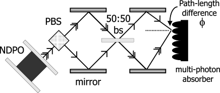
Figure 1: A strongly-pumped NDPO serves as the source, with signal, idler and pump modes interacting via a $\chi^{(2)}$— nonlinearity inside an optical cavity. Signal and idler modes are frequency degenerate and have different polarizations. External signal and idler modes are separated into different spatial paths by a polarizing beam splitter. The two modes are then combined at a 50:50 beam splitter, and are recombined at a multi-photon–absorbing recording material.

The setup for a quantum lithography experiment is illustrated in Fig. 1. We start at the NDPO source. The modes corresponding to the signal and idler have frequency $\omega$, and we denote the corresponding creation operators as $\hat{a}^{{\dagger}}_{1}$ and $\hat{a}^{{\dagger}}_{2}$. The signal and idler modes are assumed to experience linear losses characterized by the decay rate $\gamma$, which arises from transmission, absorption, and scattering losses. We assume the pump field to be a classical field of frequency $2\omega$ and of normalized amplitude denoted by $\epsilon$ (assumed to be given by a positive value). The cavity pump mode is subject to linear loss with decay rate $\gamma_{3}$, and we assume that $\gamma_{3}\gg\gamma$. The creation operator corresponding to the cavity pump mode is $\hat{a}^{{\dagger}}_{3}$. The Hamiltonian describing this system in the interaction picture can be written as,

$$\hat{H}_{I}\!=\!i\hbar\kappa\left(\hat{a}_{1}^{\dagger}\hat{a}_{2}^{\dagger}\hat{a}_{3}\!-\!\hat{a}_{1}\hat{a}_{2}\hat{a}_{3}^{\dagger}\right)+i\hbar\gamma_{3}\varepsilon\left(\hat{a}_{3}^{{\dagger}}\!-\!\hat{a}_{3}\right)+\hat{H}_{\text{loss}},$$ (1)

where $\kappa$ is the mode-coupling constant determined by the strength of the optical nonlinearity, and $\hat{H}_{\text{loss}}$ describes the interaction of the principal modes with all the reservoir modes. Light emitted by the cavity into the external signal and idler modes, assumed to have orthogonal polarizations, is separated into two spatial paths by a polarizing beam splitter. These modes are then combined at a symmetric beam splitter, and finally recombined at the multi-photon absorbing material using mirrors, such that the beams are counterpropagating at grazing incidence over the area of interest. Two classical beams incident on single-photon absorbing material would generate a fringe pattern of the form $\propto\left[1\!+\!\cos(2kx)\right]$, where $k$ denotes the optical wave number for the signal and idler modes, and $x$ denotes translation across the substrate. We shall denote the optical phase difference $2kx$ by $\phi$. When the recording medium is a $p$-photon absorber, and the illuminating beams have statistics which need not be classical, the absorption rate is given by $\sigma^{(p)}{\rm tr}\left(\hat{\rho}{\hat{E}^{+}(x)}^{p}{\hat{E}^{-}(x)}^{p}\right)$, where $\hat{\rho}$ is the density matrix for the state of the illuminating field, and $\sigma^{(p)}$ is a generalized cross-section for the process. This result holds whenever the optical field may be considered stationary, quasi-monochromatic and resonant Mollow (1968); Agarwal (1970). It can be seen that the absorption process will be strongly influenced by the statistical properties of the light Qu and Singh (1992).

II.2 Master equation and solution using the positive-$P$ distribution

Following a standard model for the NDPO, the Markovian master equation for the reduced density operator for the pump, signal and idler fields is given by Carmichael (1998); Gardiner and Zoller (2004) ,

$$\frac{\partial\hat{\rho}}{\partial t} = \frac{1}{i\hbar}\left[\hat{H}_{I},\hat{\rho}\right]+\gamma\sum_{i=1}^{2}\left(2\hat{a}_{i}\hat{\rho}\hat{a}_{i}^{{\dagger}}-\hat{a}_{i}^{{\dagger}}\hat{a}_{i}\hat{\rho}-\hat{\rho}\hat{a}_{i}^{{\dagger}}\hat{a}_{i}\right)$$ (2)

$$+\gamma_{3}\left(2\hat{a}_{3}\hat{\rho}\hat{a}_{3}^{{\dagger}}-\hat{a}_{3}^{{\dagger}}\hat{a}_{3}\hat{\rho}-\hat{\rho}\hat{a}_{3}^{{\dagger}}\hat{a}_{3}\right),$$

where $\hat{H}_{I}$ here excludes the $\hat{H}_{loss}$ term of Eq. (1), which couples the cavity modes to reservoir modes. We now map this master equation into a classical Fokker-Planck equation using the positive-$P$ representation introduced by Gardiner and Drummond Drummond and Gardiner (1980). For the current problem this representation is defined as follows,

$$\hat{\rho}\!=\!\int_{D}\prod_{i=1}^{3}d^{2}\alpha_{i}d^{2}\alpha_{i\ast}\frac{\left|\alpha_{i}\right\rangle\left\langle\alpha_{i\ast}\right|}{\left\langle\alpha_{i\ast}|\alpha_{i}\right\rangle}P\left(\vec{\alpha}\right).$$ (3)

The six variables $\alpha_{1}$,$\alpha_{1*},\alpha_{2}$,$\alpha_{2*},\alpha_{3}$ and $\alpha_{3*}$ are independent complex variables, and we have written $\vec{\alpha}\!\equiv\!\left(\alpha_{1},\alpha_{1*},\alpha_{2},\alpha_{2*},\alpha_{3},\alpha_{3*}\right)$. It should be emphasized that the asterisks in the variable indices do not correspond to complex conjugation. The complex variables $\alpha_{i}$ and $\alpha_{i*}$ correspond to the mode operators via the relations: $\hat{a}_{i}|\alpha_{i}\rangle\!=\!\alpha_{i}|\alpha_{i}\rangle$ and $\langle\alpha_{i*}|\hat{a}^{\dagger}_{i}\!=\!\alpha_{i*}\langle\alpha_{i*}|$. The distribution function $P(\vec{\alpha})$ may be assumed to have the mathematical properties of a probability density function: it is real valued, positive, and normalized to one when integrated over the full domain $D$ of $\vec{\alpha}$. For the master equation, Eq. (2), the corresponding positive-$P$ function satisfies the following,

$$\frac{\partial P}{\partial t} \!\!=\!\! \Big{[}\frac{\partial}{\partial\alpha_{1}}\!\left(\gamma\alpha_{1}\!-\!\kappa\alpha_{2\ast}\alpha_{3}\right)\!+\!\frac{\partial}{\partial\alpha_{2}}\!\left(\gamma\alpha_{2}\!-\!\kappa\alpha_{1\ast}\alpha_{3}\right)\!+\!$$ (4)

$$\frac{\partial}{\partial\alpha_{1\ast}}\!\left(\gamma\alpha_{1\ast}\!-\!\kappa\alpha_{2}\alpha_{3\ast}\right)\!+\!\frac{\partial}{\partial\alpha_{2\ast}}\!\left(\gamma\alpha_{2\ast}\!-\!\kappa\alpha_{1}\alpha_{3\ast}\right)\!+\!$$

$$\frac{\partial}{\partial\alpha_{3}}\left(\gamma_{3}\alpha_{3}+\kappa\alpha_{1}\alpha_{2}-\gamma_{3}\varepsilon\right)+$$

$$\frac{\partial}{\partial\alpha_{3\ast}}\left(\gamma_{3}\alpha_{3\ast}+\kappa\alpha_{1\ast}\alpha_{2\ast}-\gamma_{3}\varepsilon\right)+$$

$$\kappa\frac{\partial^{2}\alpha_{3}}{\partial\alpha_{1}\partial\alpha_{2}}+\kappa\frac{\partial^{2}\alpha_{3\ast}}{\partial\alpha_{1\ast}\partial\alpha_{2\ast}}\Big{]}P.$$

This has of the form of a multivariate Fokker-Planck equation Risken (1984), and the use of the positive-$P$ distribution ensures that the diffusion matrix is positive. The Langevin equations corresponding to Eq. (4) can be written as,

$$\frac{d\alpha_{1}}{dt} = -\gamma\alpha_{1}+\kappa\alpha_{2\ast}\alpha_{3}+\sqrt{\kappa\alpha_{3}}\frac{\left[\xi_{1}\left(t\right)\!+\!i\xi_{2}\left(t\right)\right]}{\sqrt{2}},$$

$$\frac{d\alpha_{2}}{dt} = -\gamma\alpha_{2}+\kappa\alpha_{1\ast}\alpha_{3}+\sqrt{\kappa\alpha_{3}}\frac{\left[\xi_{1}\left(t\right)\!-\!i\xi_{2}\left(t\right)\right]}{\sqrt{2}},$$

$$\frac{d\alpha_{3}}{dt} = -\gamma_{3}\alpha_{3}-\kappa\alpha_{1}\alpha_{2}+\gamma_{3}\varepsilon,$$

$$\frac{d\alpha_{1\ast}}{dt} = -\gamma\alpha_{1\ast}+\kappa\alpha_{2}\alpha_{3\ast}+\sqrt{\kappa\alpha_{3\ast}}\frac{\left[\xi_{3}\left(t\right)\!-\!i\xi_{4}\left(t\right)\right]}{\sqrt{2}},$$

$$\frac{d\alpha_{2\ast}}{dt} = -\gamma\alpha_{2\ast}+\kappa\alpha_{1}\alpha_{3\ast}+\sqrt{\kappa\alpha_{3\ast}}\frac{\left[\xi_{3}\left(t\right)\!+\!i\xi_{4}\left(t\right)\right]}{\sqrt{2}},$$

$$\frac{d\alpha_{3\ast}}{dt} = -\gamma_{3}\alpha_{3\ast}-\kappa\alpha_{1\ast}\alpha_{2\ast}+\gamma_{3}\varepsilon,$$ (5)

where the $\xi_{i}$ are real-valued, white-noise, stochastic variables with $\langle\xi_{j}(t)\rangle=0$ and $\langle\xi_{i}(t)\xi_{j}(t^{\prime})\rangle=\delta_{ij}\delta(t-t^{\prime})$ for all values of the indices.

Since it is assumed for the mode loss parameters that $\gamma_{3}\gg\gamma$, the pump field can be adiabatically eliminated. Setting $\dot{\alpha}_{3}=\dot{\alpha}_{3*}=0$ then leads to,

$$\alpha_{3} = \varepsilon-\frac{\kappa}{\gamma_{3}}\alpha_{1}\alpha_{2},$$

$$\alpha_{3\ast} = \varepsilon-\frac{\kappa}{\gamma_{3}}\alpha_{1\ast}\alpha_{2\ast}.$$ (6)

Substituting Eq. (II.2) into Eq. (II.2), we obtain,

$$\frac{d\alpha_{1}}{d\tau}\!\! = \!-\alpha_{1}\!+\!\frac{\left(\sigma\!-\!2\alpha_{1}\alpha_{2}\right)\alpha_{2\ast}}{n_{0}}\!+\!\sqrt{\frac{\sigma\!-\!2\alpha_{1}\alpha_{2}}{n_{0}}}\left(\frac{\xi_{1}\!+\!i\xi_{2}}{\sqrt{2}}\right)\!\!,$$

$$\frac{d\alpha_{2}}{d\tau}\!\! = \!-\alpha_{2}\!+\!\frac{\left(\sigma\!-\!2\alpha_{1}\alpha_{2}\right)\alpha_{1\ast}}{n_{0}}\!+\!\sqrt{\frac{\sigma\!-\!2\alpha_{1}\alpha_{2}}{n_{0}}}\left(\frac{\xi_{1}\!-\!i\xi_{2}}{\sqrt{2}}\right)\!\!,$$

$$\frac{d\alpha_{1\ast}}{d\tau}\!\!\! = \!\!\!\!-\alpha_{1\ast}\!\!+\!\!\frac{\left(\sigma\!\!-\!\!2\alpha_{1\ast}\alpha_{2\ast}\right)\alpha_{2}}{n_{0}}\!+\!\!\sqrt{\frac{\sigma\!\!-\!\!2\alpha_{1\ast}\alpha_{2\ast}}{n_{0}}}\left(\frac{\xi_{3}\!-\!i\xi_{4}}{\sqrt{2}}\right)\!\!,$$

$$\frac{d\alpha_{2\ast}}{d\tau}\!\!\! = \!\!\!\!-\alpha_{2\ast}\!\!+\!\!\frac{\left(\sigma\!\!-\!\!2\alpha_{1\ast}\alpha_{2\ast}\right)\alpha_{1}}{n_{0}}\!+\!\!\sqrt{\frac{\sigma\!\!-\!\!2\alpha_{1\ast}\alpha_{2\ast}}{n_{0}}}\left(\frac{\xi_{3}\!+\!i\xi_{4}}{\sqrt{2}}\right)\!\!,$$

where time has been scaled in terms of the cavity lifetime $\tau=\gamma t$. Parameter $n_{0}=2\gamma\gamma_{3}/\kappa^{2}$ is proportional to the square of the number of photons in the cavity at threshold, and sets the scale for the number of photons necessary to explore the nonlinearity of interaction. $\sigma=2\gamma_{3}\epsilon/\kappa$ is a scaled measure of the pump field amplitude relative to its value at threshold. At threshold the rates $\gamma$ and $\epsilon\kappa$ are equal, and therefore $\sigma=n_{0}$.

Using the reparametrization set out in Refs. Vyas (1992); Vyas and Singh (1995), this set of Langevin equations can be decoupled, and the dimensionality of the problem can be reduced from eight to four. We define four real-valued parameters $u_{1}$,$u_{2}$,$u_{3}$, and $u_{4}$ according to,

$$\left(\begin{array}[]{c}\alpha_{1}\\ \alpha_{2}\\ \alpha_{1*}\\ \alpha_{2*}\\ \end{array}\right)=\left(\frac{\sigma^{2}}{8n_{0}}\right)^{1/4}\left(\begin{array}[]{cccc}1&1&i&i\\ 1&1&-i&-i\\ 1&-1&-i&i\\ 1&-1&i&-i\\ \end{array}\right)\left(\begin{array}[]{c}u_{1}\\ u_{2}\\ u_{3}\\ u_{4}\\ \end{array}\right)\,.$$ (8)

The $u_{i}$ may be interpreted as scaled pseudo-quadrature variables. An exact distribution for the positive-$P$ function for the NDPO may now be written down, as presented first in Vyas and Singh (1995), valid for below-, near-, and above-threshold regimes. For $n_{0}\sim 10^{6}-10^{8}$, a typical value for laboratory systems Holliday and Singh (1986), the positive-$P$ function is given to a very good approximation by

$$P\left(\vec{u}\right) \!\!\propto\!\! \exp\Big{\{}a_{1}\left(u_{1}^{2}\!+\!u_{3}^{2}\right)\!+\!a_{2}\left(u_{2}^{2}\!+\!u_{4}^{2}\right)$$

$$-\frac{1}{2}\left[\left(u_{1}^{2}\!+\!u_{2}^{2}\!+\!u_{3}^{2}\!+\!u_{4}^{2}\right)^{2}\!+\!4\left(u_{1}^{2}\!+\!u_{3}^{2}\right)\left(u_{2}^{2}\!+\!u_{4}^{2}\right)\right]\Big{\}},$$

where $\vec{u}=\left(u_{1},u_{2},u_{3},u_{4}\right)$. Parameters $a_{1}$, $a_{2}$ correspond to the pump strength and are given by,

$$a_{1} = \sqrt{2n_{0}}\left(r-1\right),$$

$$a_{2} = -\sqrt{2n_{0}}\left(r+1\right),$$ (10)

where $r=\sigma/n_{0}=\kappa\epsilon/\gamma$. It can be seen from Eq. (II.2) that any moment of the form,

$$\left\langle u_{1}^{n_{1}}u_{2}^{n_{2}}u_{3}^{n_{3}}u_{4}^{n_{4}}\right\rangle\!=\!\int_{-\infty}^{\infty}\!\int_{-\infty}^{\infty}\!\int_{-\infty}^{\infty}\!\int_{-\infty}^{\infty}u_{1}^{n_{1}}u_{2}^{n_{2}}u_{3}^{n_{3}}u_{4}^{n_{4}}P\left(\vec{u}\right),$$

has the value zero if any of the $n_{i}$ is odd. The distribution of Eq. (II.2) can be used to evaluate the steady-state expectation values for any normally-ordered product of the field operators. In the next section, we will compute the absorption rates for multi-photon recording media, exploiting the symmetries of $P\left(\vec{u}\right)$ and making approximations valid for the different regimes of operation of the NDPO.

III Results

In this section, we compute the multi-photon absorption rates at the recording medium for a quantum-lithographic process, by computing expectation values using the positive-$P$ distribution presented in Eq. (II.2). We first propagate the signal and idler variables $\alpha_{1},\alpha_{1*}$ and $\alpha_{2},\alpha_{2*}$ through the imaging apparatus, as described in Sec. II. By interfering the signal and idler fields at a symmetric 50:50 beam splitter, the fields at the output are given by,

$$\beta_{1} = \frac{(-\alpha_{1}+i\alpha_{2})}{\sqrt{2}}$$

$$\beta_{2} = \frac{(-\alpha_{2}+i\alpha_{1})}{\sqrt{2}}$$

$$\beta_{1*} = \frac{(-\alpha_{1*}-i\alpha_{2*})}{\sqrt{2}}$$

$$\beta_{2*} = \frac{(-\alpha_{2*}-i\alpha_{1*})}{\sqrt{2}}.$$ (11)

Propagating the fields to the multi-photon recording material, the combined field, at a location corresponding to an optical phase difference of $\phi$, is given by $\alpha_{3}=(\beta_{1}e^{i\phi}+\beta_{2})$ and $\alpha_{3*}=(\beta_{1*}e^{-i\phi}+\beta_{2*})$. Substituting Eq. (III) in these expressions, we obtain,

$$\alpha_{3} = \frac{1}{\sqrt{2}}\left[\alpha_{1}(-e^{i\phi}+i)+\alpha_{2}(ie^{i\phi}-1)\right]$$

$$\alpha_{3*} = \frac{1}{\sqrt{2}}\left[\alpha_{1*}(-e^{-i\phi}-i)+\alpha_{2*}(-ie^{-i\phi}-1)\right].$$ (12)

The rate of $p$-photon absorption then is given by the average quantity,

$$I^{p}_{3}(\phi)\!=\!\langle\alpha_{3}(\vec{u})^{p}\alpha_{3*}(\vec{u})^{p}\rangle.$$ (13)

Substituting Eq. (8), we also have,

$$\alpha_{3\ast}\alpha_{3}\!\!\! = \!\!\!\frac{1}{2c^{2}}\left[\left(u_{1}\!-\!u_{2}\right)\cos\left(\frac{\phi}{2}\right)\!+\!i\left(u_{3}\!-\!u_{4}\right)\sin\left(\frac{\phi}{2}\right)\right]$$ (14)

$$\left[\left(u_{1}\!+\!u_{2}\right)\cos\left(\frac{\phi}{2}\right)\!-\!i\left(u_{3}\!+\!u_{4}\right)\sin\left(\frac{\phi}{2}\right)\right]\!\!.$$

We first evaluate the fringe pattern for a one-photon absorber, given by $I^{1}_{3}\left(\phi\right)$. Inspecting the symmetries of the positive-$P$ function, Eq. (II.2), we see that symmetries exist between the variables $u_{1}$ and $u_{3}$, as well as $u_{2}$ and $u_{4}$, so that $P(u_{1},u_{2},u_{3},u_{4})\!=\!P(u_{3},u_{2},u_{1},u_{4})$ and $P(u_{1},u_{2},u_{3},u_{4})\!=\!P(u_{1},u_{4},u_{3},u_{2})$. It follows immediately that

$$I^{1}_{3}(\phi)\!=\!r\sqrt{2n_{0}}\left(\left\langle u_{1}^{2}\rangle\!-\!\langle u_{2}^{2}\right\rangle\right),$$ (15)

and there is no dependence on $\phi$ either below or above threshold, and the illumination of the substrate is constant across the surface in the ensemble-averaged sense. Next we consider the case of multi-photon absorbing materials.

III.1 Below threshold regime

Inspecting the positive-P distribution, Eq. (II.2), for the below threshold case, $\kappa\epsilon\ll\gamma$, we find that $a_{1}$ and $a_{2}$ are large negative quantities, and the distribution can be approximated by,

$$P\left(\vec{u}\right)\!\! \approx \!\!\left(\sqrt{\frac{|a_{1}|}{\pi}}e^{-\left|a_{1}\right|u_{1}^{2}}\right)\left(\sqrt{\frac{|a_{1}|}{\pi}}e^{-\left|a_{1}\right|u_{3}^{2}}\right)$$ (16)

$$\!\!\times\left(\sqrt{\frac{|a_{2}|}{\pi}}e^{-\left|a_{2}\right|u_{2}^{2}}\right)\left(\sqrt{\frac{|a_{2}|}{\pi}}e^{-\left|a_{2}\right|u_{4}^{2}}\right).$$

For a typical NDPO with $n_{0}\sim 10^{6}$ this approximation is very good for the parameter $r$ ranging from $0$ to $0.99$. The four variables $u_{i}$ are Gaussian and independent. Their even order moments are given by

$$\left\langle u_{1}^{2k}\right\rangle = \left\langle u_{3}^{2k}\right\rangle=\frac{\left(2k\right)!}{k!\left(4\left|a_{1}\right|\right)^{k}}\;,$$

$$\left\langle u_{2}^{2k}\right\rangle = \left\langle u_{4}^{2k}\right\rangle=\frac{\left(2k\right)!}{k!\left(4\left|a_{2}\right|\right)^{k}}\;,$$ (17)

and their odd order moments vanish.

In order to compute the multi-photon absorption rates $I_{3}^{p}\left(\phi\right)$, defined by Eq. (13) and Eq. (14), a suitable grouping of terms must be found. To this end we define the function,

$$F\left(u_{i},u_{j},\phi\right)=\left[u_{i}\cos\left(\phi/2\right)-iu_{j}\sin\left(\phi/2\right)\right]^{2},$$ (18)

so that $I_{3}^{p}$ can be expressed as

$$I_{3}^{p}\left(\phi\right)\!\!\!\! = \!\!\!\!\left(r\sqrt{2n_{0}}\right)^{p}\sum_{k=0}^{p}\binom{p}{k}\left(-1\right)^{p-k}$$ (19)

$$\times\left\langle F\left(u_{1},u_{4},\phi\right)^{k}\right\rangle\left\langle F\left(u_{2},u_{3},\phi\right)^{p-k}\right\rangle\!.$$

We exploit the fact that the $u_{i}$ are not coupled, to evaluate the moments of separable sums independently. Since the pairs of variables $u_{1}$ and $u_{3}$, and $u_{2}$ and $u_{4}$, share the same distribution, we also conclude

$$\left(-1\right)^{p-k}\left\langle F\left(u_{2},u_{3},\phi\right)^{p-k}\right\rangle = \left\langle F\left(u_{3},u_{2},\phi+\pi\right)^{p-k}\right\rangle$$

$$= \left\langle F\left(u_{1},u_{4},\phi+\pi\right)^{p-k}\right\rangle.$$

Expanding an arbitrary moment $k$ of $F\left(u_{1},u_{4},\phi\right)$ we find

$$\left\langle F\left(u_{1},u_{4},\phi\right)^{k}\right\rangle\! = \!\sum_{l=0}^{k}\binom{2k}{2l}\left\langle u_{1}^{2l}\right\rangle\left\langle u_{4}^{2k-2l}\right\rangle\left(-1\right)^{\left(k-l\right)}$$ (20)

$$\times\cos^{2l}\left(\phi/2\right)\sin^{2k-2l}\left(\phi/2\right).$$

By substituting the expressions for the even moments $u_{1}$ and $u_{4}$ given above, and the form of parameters $a_{1}$ and $a_{2}$ defined by Eq. (II.2), this sum can be evaluated as,

$$\left\langle F\left(u_{1},u_{4},\phi\right)^{k}\right\rangle\!=\!\frac{\left(2k\right)!}{k!4^{k}\left(\sqrt{2n_{0}}\right)^{k}\left(1-r^{2}\right)^{k}}\left[r+\cos\left(\phi\right)\right]^{k}.$$ (21)

Using these relations, we arrive at a compact expression for the $p$-photon absorption rate,

$$I_{3}^{p}(\phi) = \left[\frac{r}{4\left(1-r^{2}\right)}\right]^{p}p!\sum_{k=0}^{p}\frac{\left(2k\right)!\left(2p-2k\right)!}{k!^{2}\left(p-k\right)!^{2}}$$ (22)

$$\times\left[r+\cos\left(\phi\right)\right]^{k}\left[r-\cos\left(\phi\right)\right]^{\left(p-k\right)}.$$

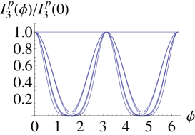
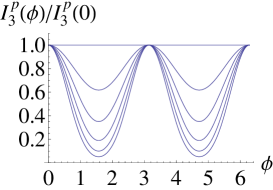
(a) (b)

Figure 2: Plots (a) and (b) show the absorption rates $I_{3}^{p}(\phi)$, scaled between 0 and 1, for $p=1,\cdots,6$. It is assumed that the NDPO is operated below threshold, with pump parameter $r=0.15$ in (a) and $r=0.9$ in (b). As $p$ increases the corresponding fringe patterns become better defined.

Looking in detail at the form of the absorption rates $I_{3}^{p}(\phi)$ in Eq. (22) we see for the following. For the $p=1$ case, the absorption rate is constant and no fringe pattern is created, as already seen following Eq. (15). For the case of $p\geq 2$, $I_{3}^{p}(\phi)$ is given as a sum of even powers of $\cos(\phi)$. The corresponding fringe pattern therefore has terms with periods corresponding to $\cos(2n\phi)$ where $2n\leq p$. As $p$ increases, there is a greater contribution from higher power terms with sharper interference patterns. The fringe patterns for the cases of $p=1,\cdots,6$ are plotted in Fig. 2(a) and (b), for the pump parameter $r=0.15$ and $0.9$ respectively.

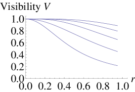
Figure 3: The visibility, defined by $V=\left[I^{p}_{3}(\phi_{\rm max})\!-\!I^{p}_{3}(\phi_{\rm min})\right]/\left[I^{p}_{3}(\phi_{\rm max})\!+\!I^{p}_{3}(\phi_{\rm min})\right]$ and normalized between 0 and 1, is plotted for $p=2,\cdots,6$ as a function of pump parameter $r$ for the NDPO operating below threshold.

Fig. 3 shows fringe visibilities as $r$ ranges from 0 to 0.95. It is seen that for every case with $p\geq 2$, the visibilities are close to 1 when the NDPO is operated far below threshold, but as the pump power is increased the visibilities fall steadily. In a lithographic process, it is possible to compensate for unwanted constant exposure by using a substrate with greater depth, and visibilities greater than 0.2 are often considered adequate in practice. This criterion is satisfied in all cases considered here with $p\geq 2$. Making a comparison with the case of an OPA source reported in the earlier work of Agarwal, et al., in Ref. Agarwal et al. (2007), we find the following. Eq. (22) is listed explicitly in Table 1 of Appendix A for the cases of $p=1,\cdots,6$. Inspecting Eqs. (19-22) of Ref. Agarwal et al. (2007) we find the formulae for the multi-photon absorption rates identical on identifying $r$ in current analysis and $\tanh(G)$ in the analysis of Agarwal, et al., for which $G$ represents the single-pass gain for the OPA. The range for parameter $r$ for the NDPO below threshold (from $0\to 1_{-}$), corresponds to values of parameter $G$ for the OPA from $0\to\infty$. Visibilities for the sub-threshold NDPO are listed in Table 2 of Appendix A for $p=1,\cdots,6$, which agree with the results reported for the OPA across the corresponding range for the parameter $G$.

III.2 Near and above threshold regime

As the NDPO is pumped more strongly and passes through threshold, pump rate $r$ exceeds unity, the nature of the positive-$P$ distribution changes significantly. Inspecting the governing parameters $a_{1}$ and $a_{2}$, defined by Eq. (II.2), we see that while $a_{2}$ continues to take large negatives values of increasing size as $r$ increases, $a_{1}$ is zero at threshold and takes positive values for $r>1$. The positive-$P$ distribution, given by Eq. (II.2), may now be well approximated by the expression below, which is valid both near and far above threshold for values of $n_{0}$ greater than $10^{4}$ (Vyas and Singh (2006)),

$$P\left(\vec{u}\right)\!\!\! \simeq \!\!\!\left(\sqrt{\frac{\left|a_{2}\right|}{\pi}}e^{-\left|a_{2}\right|u_{2}^{2}}\right)\left(\sqrt{\frac{\left|a_{2}\right|}{\pi}}e^{-\left|a_{2}\right|u_{4}^{2}}\right)$$ (23)

$$\times \!\!\!\left(Ne^{-\frac{1}{2}\left(u_{1}^{2}+u_{3}^{2}-a_{1}\right)^{2}}\right),$$

where $N$ denotes a normalization factor for the $u_{1}$,$u_{3}$ component, defined by

$$N\!=\!\frac{\sqrt{2}}{\left[\pi^{3/2}{\rm erfc}\left(-a_{1}/\sqrt{2}\right)\right]},$$

and ${\rm erfc(z)}\equiv({2}/{\sqrt{\pi}})\int_{z}^{\infty}e^{-s^{2}}ds$ is the complementary error function. It can be seen that variables $u_{2}$ and $u_{4}$ are independent Gaussian variables with pump parameter $a_{2}$ in the below-threshold regime. However, variables $u_{1}$ and $u_{3}$ with pump parameter $a_{1}$ are now strongly coupled. As a consequence, the decomposition given by Eq. (19), used to evaluate $I_{p}(\phi)$ in the below-threshold case, can no longer be applied.

To proceed, in this case we look in detail at the moments for the $u_{i}$ that arise in computing $I_{p}(\phi)$ above threshold. The moments for the Gaussian variables $u_{2}$ and $u_{4}$ are as before given by Eq. (17). By reparametrizing $u_{1}$ and $u_{3}$ in polar coordinates, it follows that,

$$\left\langle u_{1}^{2s}u_{3}^{2t}\right\rangle\!\left\langle u_{2}^{2m}\right\rangle\!\left\langle u_{4}^{2n}\right\rangle\!\! = \!\!R\left(2s\!+\!2t\!+\!1,a_{1}\right)B\left(s\!+\!\frac{1}{2},t\!+\!\frac{1}{2}\right)$$ (24)

$$\times \!\!2N\frac{\left(2m\right)!}{m!\left(4\left|a_{2}\right|\right)^{m}}\frac{\left(2n\right)!}{n!\left(4\left|a_{2}\right|\right)^{n}}.$$

$B\left(\cdot,\cdot\right)$ here denotes the Beta function, defined by $B\left(S,T\right)\equiv\Gamma\left(S\right)\Gamma\left(T\right)/\Gamma\left(S+T\right)$, and arises from the integration over the angular component associated with $u_{1}$ and $u_{3}$. The integration over the remaining radial component leads to the $R\left(\cdot\right)$ contribution, defined by, $R\left(S,a_{1}\right)\equiv\int_{0}^{\infty}\rho^{S}e^{-\frac{1}{2}\left(\rho^{2}-a_{1}\right)^{2}}d\rho$. Writing,

$$R\left(2s\!+\!2t\!+\!1,a_{1}\right)\!\! = \!\!\int_{0}^{\infty}\!\!\!\rho^{2s+2t-1}\left(\rho^{2}\!-\!a_{1}\right)e^{-\frac{1}{2}\left[\rho^{2}-a_{1}\right]^{2}}d\rho$$ (25)

$$+ a_{1}R\left(2s\!+\!2t\!-\!1,a_{1}\right),$$

for $s+t\geq 1$, and integrating by parts,

$$\int_{0}^{\infty}\rho^{2s+2t-1}\left(\rho^{2}\!-\!a_{1}\right)e^{-\frac{1}{2}\left[\rho^{2}-a_{1}\right]^{2}}d\rho$$

$$=\begin{cases}\frac{1}{2}e^{-\frac{1}{2}a_{1}^{2}}\,\,\,&(\rm{if}\,\,s+t=1),\\ \left(s\!+\!t\!-\!1\right)R\left(2s\!+\!2t\!-\!3,a_{1}\right)\,\,\,&(\rm{if}\,\,s+t>1),\end{cases}$$ (26)

we get a recursion relation for $R\left(\cdot\right)$. Here we list first few radial functions,

$$R\left(1,a_{1}\right)\!\!\! = \!\!\!\frac{1}{2\pi N}$$

$$R\left(3,a_{1}\right)\!\!\! = \!\!\!\frac{1}{2}\exp\left(-\frac{1}{2}a_{1}{}^{2}\right)+a_{1}\frac{1}{2\pi N}$$

$$R\left(5,a_{1}\right)\!\!\! = \!\!\!\frac{a_{1}}{2}\exp\left(-\frac{1}{2}a_{1}{}^{2}\right)+(1+a_{1}{}^{2})\frac{1}{2\pi N}$$

$$R\left(7,a_{1}\right)\!\!\! = \!\!\!\left(1+\frac{1}{2}a_{1}^{2}\right)\exp\left(-\frac{1}{2}a_{1}{}^{2}\right)+\left(3a_{1}+a_{1}^{3}\right)\frac{1}{2\pi N}$$

$$R\left(9,a_{1}\right)\!\!\! = \!\!\!\left(\!\frac{5}{2}a_{1}\!+\!\frac{1}{2}a_{1}{}^{3}\!\right)\exp\left(\!-\frac{1}{2}a_{1}{}^{2}\!\right)\!+\!\frac{\left(3\!+\!6a_{1}{}^{2}\!+\!a_{1}{}^{4}\right)}{2\pi N}$$

Below threshold ($r=\kappa\epsilon/\gamma<1$), the parameter $a_{1}$ is negative. It is zero at threshold ($r=\kappa\epsilon/\gamma=1$), and positive above threshold ($r=\kappa\epsilon/\gamma>1$). As $a_{1}$ increases from negative to positive values the NDPO goes through a phase transition, and the intensities of the signal and idler modes increase very rapidly. For a typical value of $n_{0}=10^{6}-10^{8}$, the region for phase transition is very narrow and a small change in $r$ from $0.99\to 1.01$ changes the statistics of the NDPO dramatically Vyas and Singh (1995, 2006). In this region, we find that the visibility for $p$-photon absorption changes from the below-threshold to the above-threshold behavior.

For the NDPO operating much above threshold ($a_{1}>>1$), we can considerably simplify the expression for $I_{3}^{p}(\phi)$. It follows from Eqs. (24) and (III.2) that $\left\langle u_{1}^{2s}u_{3}^{2t}\right\rangle\simeq B\left(s+1/2,t+1/2\right)a_{1}^{s+t}/\pi$. Since powers of $n_{0}$ appear only in the denominator for moments of $u_{2}$ and $u_{4}$, and in the expansion of $I_{p}(\phi)$ the powers of the variables $u_{i}$ satisfy $s+t+m+n=p$ , it follows that all contributions from variables $u_{2}$ and $u_{4}$ can be neglected. Within this approximation,

$$\alpha_{3}^{p}\alpha_{3\ast}^{p}\simeq\left(r\sqrt{2n_{0}}\right)^{p}\left[u_{1}^{2}\cos^{2}\left(\phi/2\right)+u_{3}^{2}\sin^{2}\left(\phi/2\right)\right]^{p},$$

and we find the expectation value,

$$I_{p}\left(\phi\right)\!\!\!\! = \!\!\!\!\left(r\sqrt{2n_{0}}\right)^{p}\!\!\;\;\sum_{s=0}^{p}\binom{p}{s}\left\langle u_{1}^{2s}u_{3}^{2p-2s}\right\rangle$$ (28)

$$\times\cos^{2s}\!\left(\frac{\phi}{2}\right)\sin^{2p-2s}\!\left(\frac{\phi}{2}\right)$$

$$= \left(\frac{a_{1}r\sqrt{2n_{0}}}{8}\right)^{p}\sum_{s=0}^{p}\frac{\left(2s\right)!\left(2p-2s\right)!}{s!^{2}\left(p-s\right)!^{2}}$$

$$\,\,\,\times\,\,\,\left[1+\cos\left(\phi\right)\right]^{s}\!\left[1-\cos\left(\phi\right)\right]^{p-s}.$$

The $p$-photon absorption rates for much above threshold, are therefore seen to generate fringe patterns of a form independent of the strength of the pump. Fig. 4 shows how the fringe visibility changes near the threshold regime for the 2-photon case. Note that as $r$ changes from $0.97\to 1.03$ the parameter $a_{1}$ changes from $-42\to+42$. As expected, much above threshold the visibility is almost constant.

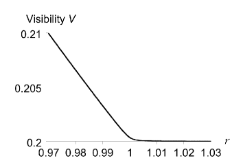
Figure 4: The visibility for $p=2$ versus pump parameter $r$ as operation of the NDPO changes from below threshold to the above threshold regime for $n_{0}=10^{6}$.

IV Discussion

In conclusion, we have found that a NDPO source can be used to generate fringe patterns with an effective wavelength half that for the signal and idler modes which interfere at the recording media, when a $p$-photon absorption process is available with $p\geq 2$. These fringe patterns have high visibility, falling from $1$ at low pump power, to asymptotic values of $0.2$ or greater at high pump power. Above threshold, the forms of the fringe patterns are insensitive to the strength of the pump, whereas below threshold, the forms of the fringe patterns depend on the pump power, and tend towards the asymptotic case as the NDPO threshold is approached. Comparing with the results reported in Ref. Agarwal et al. (2007), we find that the fringe patterns generated using an NDPO operating below threshold ($r$ from $0\to 1_{-}$) are similar to fringe pattern generated by an OPA operated with a corresponding gain ($G$ from $0\to\infty$) . In the latter case there is no cavity and no above threshold regime, and the process of optical parametric amplification occurs in propagating modes. This result is perhaps surprising, since the earlier analysis of Ref. Agarwal et al. (2007) disregards photon losses, and uses a single-mode analysis by ignoring all but one down converted spatial mode. The NDPO source has some experimental advantages. The signal and idler modes at the outputs of the NDPO are collimated because of the use of a cavity, and higher-powers can be obtained than is the case for the OPA, both of which are important in light of the small cross-sections for typical multi-photon absorption processes. Collimated, high-power, outputs also increase the speed at which a substrate may be imaged — a critical factor in the mass production of, say, computer chips. Finally, the reparameterization of the dynamics of the NDPO in terms of the four pseudo-quadrature variables $u_{i}$ above, sheds some light on why the change in fringe patterns and visibilities are observed. Far-below threshold, all four of the $u_{i}$ contribute approximately equally to the absorption process, and behave as independent parameters. As the pump power is increased, and threshold is approached, parameter $a_{1}$ tends to $0$. Since $a_{1}$ appears in the denominator of each of the moments of variables $u_{1}$ and $u_{3}$, $u_{1}$ and $u_{3}$ make a growing contribution compared to $u_{2}$ and $u_{4}$. Above threshold, variables $u_{1}$ and $u_{3}$ make the primary contribution to the absorption process, and the effects of $u_{2}$ and $u_{4}$ can be neglected. Variables $u_{1}$ and $u_{3}$ are also strongly coupled in this regime. The analysis of this paper also contributes compact general formulae for the multi-photon absorption rates, Eq. (22) and Eq. (28).

Appendix A Fringe patterns below threshold

Based on the general formula for the absorption rates below threshold, Eq. (22), the following tables list explicitly the absorption rates, and the visibilities for the corresponding fringe patterns, for $p$-photon absorbers with $p$ ranging from 1 to 6.

Table 1: $p$-photon absorption rates as a function of the optical-path-length difference $\phi$ and the pump parameter $r$, varying from far below to near threshold (from 0 to approximately 0.99).

$p$	$I_{3}^{p}(\phi)$
$1$	$\frac{r^{2}}{\left(1-r^{2}\right)}$
$2$	$\frac{r^{2}}{\left(1-r^{2}\right)^{2}}\left[\cos^{2}(\phi)+2r^{2}\right]$
$3$	$\frac{3r^{4}}{\left(1-r^{2}\right)^{3}}\left[3\cos^{2}(\phi)+2r^{2}\right]$
$4$	$\frac{3r^{4}}{\left(1-r^{2}\right)^{4}}\left[3\cos^{4}(\phi)+24r^{2}\cos^{2}(\phi)+8r^{4}\right]$
$5$	$\frac{15r^{6}}{\left(1-r^{2}\right)^{5}}\left[15\cos^{4}(\phi)+40r^{2}\cos^{2}(\phi)+8r^{4}\right]$
$6$	$\frac{45r^{6}}{\left(1-r^{2}\right)^{6}}\left[5\cos^{6}(\phi)+90r^{2}\cos^{4}(\phi)+120r^{4}\cos^{2}(\phi)+16r^{6}\right]$

Table 2: The visibilities, defined by $V=\left[I^{p}_{3}(\phi_{\rm max})\!-\!I^{p}_{3}(\phi_{\rm min})\right]/\left[I^{p}_{3}(\phi_{\rm max})\!+\!I^{p}_{3}(\phi_{\rm min})\right]$ and normalized between 0 and 1, for the fringe patterns with a $p-$photon absorbing recording material. The third column lists the limiting values for the visibilities as the pump parameter $r$ ranges from far below to near threshold (from 0 to approximately 0.99).

$p$	Visibility $V(r)$	$V(0^{+})\rightarrow V(1^{-})$
$1$	$0$	—
$2$	$1-\frac{4r^{2}}{\left[1+4r^{2}\right]}$	$1\rightarrow 0.20$
$3$	$1-\frac{4r^{2}}{\left[3+4r^{2}\right]}$	$1\rightarrow 0.43$
$4$	$1-\frac{16r^{4}}{\left[3+24r^{2}+16r^{4}\right]}$	$1\rightarrow 0.63$
$5$	$1-\frac{16r^{4}}{\left[15+40r^{2}+16r^{4}\right]}$	$1\rightarrow 0.77$
$6$	$1-\frac{32r^{6}}{\left[5+90r^{2}+120r^{4}+32r^{6}\right]}$	$1\rightarrow 0.87$

References

- Boto et al. (2000) A. N. Boto, P. Kok, D. S. Abrams, S. L. Braunstein, C. P. Williams, and J. P. Dowling, Phys. Rev. Lett. 85, 2733 (2000).
- Agarwal et al. (2001) G. S. Agarwal, R. W. Boyd, E. M. Nagasako, and S. J. Bentley, Phys. Rev. Lett. 86, 1389 (2001).
- D’Angelo et al. (2001) M. D’Angelo, M. V. Chekhova, and Y. Shih, Phys. Rev. Lett. 87, 013602 (2001).
- Boyd et al. (2005) R. W. Boyd, H. J. Chang, H. Shin, and C. O’Sullivan-Hale, in Quantum Communications and Quantum Imaging III (SPIE, San Diego, CA, 2005), vol. 5893, pp. 58930G.1–58930G.4.
- Fukutake (2005) N. Fukutake, Journal of Modern Optics 53, 719 (2005).
- Agarwal et al. (2007) G. S. Agarwal, K. W. Chan, R. W. Boyd, H. Cable, and J. P. Dowling, J. Opt. Soc. Am. B 24, 270 (2007).
- Tsang (2007) M. Tsang, Phys. Rev. A 75, 043813 (2007).
- Sciarrino et al. (2008) F. Sciarrino, C. Vitelli, F. De Martini, R. Glasser, H. Cable, and J. P. Dowling, Phys. Rev. A 77, 012324 (2008).
- Kok et al. (2001) P. Kok, A. N. Boto, D. S. Abrams, C. P. Williams, S. L. Braunstein, and J. P. Dowling, Phys. Rev. A 63, 063407 (2001).
- Hong et al. (1987) C. K. Hong, Z. Y. Ou, and L. Mandel, Phys. Rev. Lett. 59, 2044 (1987).
- Vyas and Singh (1989) R. Vyas and S. Singh, Phys. Rev. A 40, 5147 (1989).
- Vyas (1992) R. Vyas, Phys. Rev. A 46, 395 (1992).
- Vyas and Singh (1995) R. Vyas and S. Singh, Phys. Rev. Lett. 74, 2208 (1995).
- Vyas and Singh (2006) R. Vyas and S. Singh, in ICQO, edited by J. Banerji, P. K. Panigrahi, and R. P. Singh (Macmillan India Ltd., Delhi, Ahemdabad, India, 2006).
- Drummond and Gardiner (1980) P. D. Drummond and C. W. Gardiner, J. Phys. A 13, 2353 (1980).
- Carmichael (2008) H. J. Carmichael, Statistical Methods in Quantum Optics 2. Non-Classical Fields., vol. 2 (Springer-Verlag, Berlin, Heidelberg, 2008), 1st ed.
- Gardiner and Zoller (2004) C. W. Gardiner and P. Zoller, Quantum Noise, A Handbook of Markovian and Non-Markovian Quantum Stochastic Methods with Applications to Quantum Optics (Springer, Berlin, Heidel, New York, 2004), 3rd ed.
- Mollow (1968) B. R. Mollow, Phys. Rev. 175, 1555 (1968).
- Agarwal (1970) G. S. Agarwal, Phys. Rev. A 1, 1445 (1970).
- Qu and Singh (1992) Y. Qu and S. Singh, Optics Communications 90, 111 (1992), ISSN 0030-4018.
- Carmichael (1998) H. J. Carmichael, Statistical Methods in Quantum Optics 1. Master Equations and Fokker-Plank Equations., vol. 1 (Springer-Verlag, Berlin, Heidelberg, 1998), 1st ed.
- Risken (1984) H. Risken, The Fokker-Planck Equation, Methods of Solution and Applications, vol. 1 (Springer-Verlag, Berlin, Heidelberg, New York, Tokyo, 1984).
- Holliday and Singh (1986) G. S. Holliday and S. Singh, Optics Communications 62, 289 (1986).