Two dimensional frustrated magnets in high magnetic field

Abstract

Frustrated magnets in high magnetic field have a long history of offering beautiful surprises to the patient investigator. Here we present the results of extensive classical Monte Carlo simulations of a variety of models of two dimensional magnets in magnetic field, together with complementary spin wave analysis. Striking results include (i) a massively enhanced magnetocaloric effect in antiferromagnets bordering on ferromagnetic order, (ii) a route to an $m=1/3$ magnetization plateau on a square lattice, and (iii) a cascade of phase transitions in a simple model of AgNiO₂.

1 Introduction

It is precisely the feature that makes frustrated magnets so compelling — the multitude of groundstates available — that also makes them so difficult to study, especially if we take in account the extra contribution of an external magnetic field. In this article we present a snapshot of ongoing work on several experimentally motivated models of two–dimensional frustrated magnets in high magnetic field. Our main tool will be classical Monte Carlo simulation, but where the standard local update Metropolis algorithm is augmented by a parallel tempering scheme [1], which greatly improves the ergodicity of the method. Simulation results will also be compared with simple mean field theories and classical spinwave calculations.

One concept that will be used throughout this work is the magnetocaloric effect (MCE), $\theta_{MCE}={\frac{\partial T}{\partial H}\mid}_{S}$, the rate of change of temperature of the system with applied magnetic field at constant entropy. This quantity is useful as a tool for identifying phase transitions in both simulation and experiment, and forms the basis for magnetic refrigeration.

2 The $J_{1}$-$J_{2}$ Heisenberg model on a square lattice

The first model we consider is the Heisenberg model on a square lattice with additional $2^{nd}$-neighbour ($J_{2}$) bonds

$$H=J_{1}\sum_{\langle ij\rangle_{1}}\textbf{S}_{i}.\textbf{S}_{j}+J_{2}\sum_{\langle ij\rangle_{2}}\textbf{S}_{i}.\textbf{S}_{j}-h\sum_{i}S^{z}_{i}.$$ (1)

Despite its apparent simplicity, this is a very interesting model, and is thought to describe two new classes of oxide compounds [2, 3]. The classical phase diagram in zero field is shown in Fig. 2. The quantum phase diagram and finite field properties of the spin-$1/2$ quantum model have been extensively investigated for both antiferromagnetic (AF) [4] and ferromagnetic (FM) [5, 6, 7, 8] $J_{1}$. New quantum phases are found in the highly frustrated regions where $|J_{1}|=2J_{2}$. Here we explore the role of thermal fluctuations and finite magnetic field for these parameter sets.

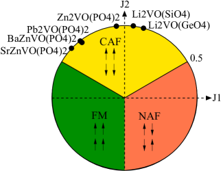
Figure 1: (Colour online) Classical phase diagram of the $J_{1}$-$J_{2}$ Heisenberg model. Parameters for quasi-2D vanadates are taken from [7].

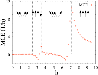
Figure 2: (Colour online) MCE of the classical $J_{1}$-$J_{2}$ Heisenberg model for $J_{1}=1$, $J_{2}=0.5$ ($T=0.01$), showing successive phase transitions. $T$ and $h$ are measured in units of $J_{1}$. The MCE is normalised to that of an ideal paramagnet.

Considering first AF $J_{1}>0$, in Fig. 2 we present the MCE for $J_{1}=1$, $J_{2}=0.5$, as determined by classical MC simulation for a cluster of $N=24\times 24$ spins at $T=0.01$. Binned data from $\sim 2\times 10^{6}$ MC steps of simulation, preceded by $\sim 6\times 10^{6}$ MC steps of thermalization, were analysed using a jackknife procedure. Analysis reveals four distinct phases, the most striking feature being a $m=1/2$ plateau (c.f. [9]).

The MCE also shows interesting structure within the collinear AF phase for FM $J_{1}<0$, approaching the classical critical point $J_{1}=-2J_{2}$, as shown in Fig. 3. Here the high degeneracy in the spin wave spectrum shows up as a massive enhancement in the MCE at low fields, also discussed for quantum spins in [7].

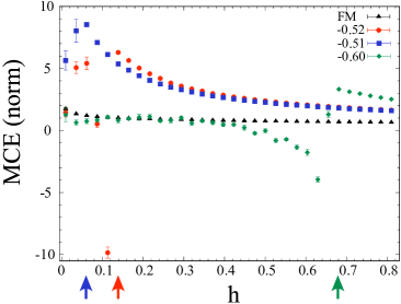
Figure 3: (Colour online). MCE of the $J_{1}$-$J_{2}$ Heisenberg model on a square lattice for different ratios of $J_{2}/J_{1}$ ($J_{1}<0$), showing a massive enhancement near the transition from collinear $(\pi,0)$ Néel AF to FM at $J_{2}/J_{1}=-0.5$.Arrows show rough values of the saturation field in each case. Results are for $24\times 24$ spins, at $T=0.01$, normalised to the maximum value of the MCE in a nearest-neighbour Heisenberg AF. $T$ and $h$ are measured in units of $J_{1}$.

3 The $J_{1}$-$J_{2}$-$J_{3}$ Heisenberg model on a square lattice

A new series of layered Dion-Jacobi compounds containing spin-$1/2$ Cu($3d^{9}$) ions on a square lattice have recently been discovered [3]. These materials are believed to have FM nearest neighbour exchange $J_{1}$, but not all of their properties can be reconciled with a simple $J_{1}$-$J_{2}$ model. In particular (CuBr)Sr₂Nb₃O₁₀ exhibits an unexpected $m=1/3$ magnetization plateau [10]. This has motivated us to consider the quantum and classical properties of Eq. 1 with additional AF third neighbour interaction $J_{3}$.

So far as classical MC simulations are concerned, our main results are summarised in Fig. 4. A clear $m=1/3$ plateau is found for $J_{1}=-1$, $J_{2}=1.0$, $J_{3}=0.5$. The classical $h$-$T$ phase diagram clearly has much in common with that for the nearest-neighbour Heisenberg AF on a triangular lattice [11]. The $m=1/3$ plateau is also observed in exact diagonalization calculations for the equivalent spin-$1/2$ $J_{1}$-$J_{2}$-$J_{3}$ model [12]. These results clearly suggest that this model deserves further study, both as a “toy model” for (CuBr)Sr₂Nb₃O₁₀ and as an interesting problem in its own right.

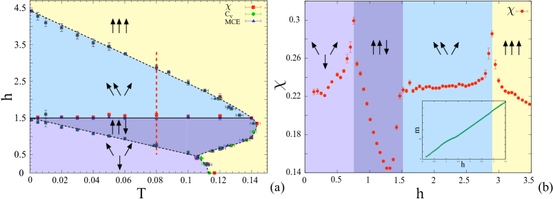
Figure 4: (Colour online.) Left Panel : Magnetic phase diagram for the classical $J_{1}$-$J_{2}$-$J_{3}$ Heisenberg model on a $24\times 24$ site square lattice, for $J_{1}=-1$, $J_{2}=1$, $J_{3}=0.5$. Points are taken from simulation results for magnetic susceptibility $\chi$, heat capacity $C_{V}$ and MCE. The vertical dashed line represents a cut at $T=0.08$. Right Panel : the magnetic susceptibility on this cut. The inset displays the average magnetization revealing the $m=1/3$ plateau. $T$ and $h$ are measured in units of $J_{1}$.

4 The easy-axis $J_{1}$-$J_{2}$ Heisenberg model on a triangular lattice

The metallic layered silver nickelate 2H-AgNiO₂ has been argued [13] to offer realisation of a spin-$1$ easy-axis AF on a triangular lattice with competing AF $J_{2}$ interactions

$$H=J_{1}\sum_{\langle ij\rangle_{1}}\textbf{S}_{i}.\textbf{S}_{j}+J_{2}\sum_{\langle ij\rangle_{2}}\textbf{S}_{i}.\textbf{S}_{j}-D\sum_{i}(S^{z}_{i})^{2}-h\sum_{i}S^{z}_{i}$$ (2)

We have investigated the high field properties of Eq. 2 with ratio of parameters $J_{1}=1.0$, $J_{2}=0.25$ and $D=0.06$ taken from preliminary fits to experiment [14]. For these parameters, the classical ground state of Eq. 2 is a two-sublattice collinear Néel state with ${\bf q}=(0,\pi)$. A natural expectation would be that, in applied magnetic field, this would undergo a 1^st order spin flop transition into a canted two-sublattice state with the same wave number. However our results support a very different scenario.

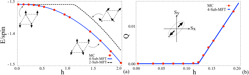
Figure 5: (Colour online) Left Panel : Ground state energies of Eq. 2 in 2-sublattice (dashed line) and 4-sublattice mean field approximations (blue line), together with results of classical MC simulation at $T=1\times 10^{-4}$ (red points). Simulation results follow the 4-sublattice solution for $h\geq 0.12$, avoiding the 2-sublattice spin-flop for $h=1.1$. Right Panel : The quadrupole moment Q, showing a continuous transition into a state with transverse order.

In Fig. 5-(a) we show results of classical MC simulations of Eq. 2, compared with a mean field theory (MFT) of the 2-sublattice spin-flop transition, and a 4-sublattice MFT. The 2-sublattice theory predicts a first order spin flop transition at $h=1.1$. However a spin wave with ${\bf q}=(\pi,\frac{\sqrt{3}\pi}{3})$ becomes soft at the much lower field of $h=0.12$, precipitating a 2^nd order transition into a 4-sublattice “supersolid” state with both transverse order and broken translational symmetry. We can identify this transition using the quadrupole moment

$$Q=\sqrt{Q_{x^{2}-y^{2}}^{2}+Q_{xy}^{2}}\qquad Q_{x^{2}-y^{2}}=\frac{1}{N}\sum_{i}(S^{x}_{i})^{2}-(S^{y}_{i})^{2}\qquad Q_{xy}=\frac{1}{N}\sum_{i}2S_{i}^{x}S^{y}_{i}$$ (3)

shown in Fig. 5-(b). We have checked in interacting spin wave theory that this “supersolid” scenario also holds for quantum spins. Our preliminary results for the global $h$-$T$ phase diagram also suggest that this supersolid state is superseded by cascade of phase transitions at higher field. These will be reported elsewhere.

References

References

- [1] Hukushima K and Nemoto K 1995 J. Phys. Soc. Jpn. 65 1604
- [2] Kaul E et al 2004 J. Magn. Magn. Mater. 272-276 922–3
- [3] Kageyama H et al 2005 J. Phys. Soc. Jpn. 74 1702–5
- [4] Misguich G and Lhuillier C 2005 in “Frustrated Spin Systems” ed H T Diep (Singapore: World Scientific)
- [5] Shannon N et al 2004 Eur. Phys. J. B 38 599–616
- [6] Shannon N et al 2006, Phys. Rev. Lett. 96 27213
- [7] Schmidt B et al 2007 Phys. Rev. B 76 125113
- [8] Thalmeier P et al 2008 Phys. Rev. B 77 10441
- [9] Zhitomirsky M et al 2000 Phys. Rev. Lett. 85 3269–72
- [10] Tsujimoto Y et al 2007 J. Phys. Soc. Jpn. 76 063711
- [11] Miyashita S 1986 J. Phys. Soc. Jpn. 55 3605–17
- [12] Sindzingre P et al 2009 J. Phys.: Conf. Ser. 145 012048
- [13] Wawrzynska E et al 2007 Phys. Rev. Lett. 99 157204
- [14] Wheeler E M et al 2009 Phys. Rev. B 79 104421