Polygamy of Distributed Entanglement

Abstract

While quantum entanglement is known to be monogamous (i.e. shared entanglement is restricted in multi-partite settings), here we show that distributed entanglement (or the potential for entanglement) is by nature polygamous. By establishing the concept of one-way unlocalizable entanglement (UE) and investigating its properties, we provide a polygamy inequality of distributed entanglement in tripartite quantum systems of arbitrary dimension. We also provide a polygamy inequality in multi-qubit systems, and several trade offs between UE and other correlation measures.

I Introduction

Quantum entanglement is a non-local quantum correlation providing a lot of useful applications in the field of quantum communications and computations such as quantum teleportation and quantum key distribution tele ; qkd1 ; qkd2 . This important role of quantum entanglement has stimulated intensive study in both way of its quantification and qualification.

One of the essential differences of quantum correlations (especially, quantum entanglement) from other classical ones is that it cannot be freely shared among the parties in multipartite quantum systems. In particular, a pair of components that are maximally entangled cannot share entanglement CKW ; ov nor classical correlations KW with any part of the rest of the system, hence the term Monogamy of Entanglement (MoE) T04 . Monogamy of entanglement was shown to have a complete mathematical characterization for multi-qubit systems ov using a certain entanglement measures, the concurrence ww .

Whereas MoE shows the restricted sharability of multi-party quantum entanglement, the distribution of entanglement, or Entanglement of Assistance (EoA) d ; cohen in multipartite quantum systems was shown to have a dually monogamous (or Polygamous) property. Using Concurrence of Assistance (CoA) lve as the measure of distributed entanglement, it was also shown that whereas monogamy of entanglement inequalities provide an upper bound for bipartite sharability of entanglement in a multipartite system, the same quantity provides a lower bound for distribution of bipartite entanglement in a multipartite system gbs . In this paper, by introducing the concept of One-way Unlocalizable Entanglement (UE), we provide a polygamy inequality of entanglement in tripartite quantum systems of arbitrary dimension using entropic entanglement measure. Based on the functional relation between concurrence and entropic measure in two-qubit systems, we provide a polygamy inequality in multi-qubit systems. We also provide several trade offs between UE and other correlations such as EoA, and localizable entanglement.

The paper is organized as follows. In Sec. II, we provide the definition of UE, and its basic properties. In Sec. III, we provide a polygamy inequality of distributed entanglement in tripartite quantum systems in terms of entropy and EoA. In Sec. IV, we generalize the polygamy inequality of entanglement into multi-qubit systems, and provide a more tight polygamy inequality for three-qubit systems. In Sec. V, we provide several trade offs between UE and other correlations, and we summarize our results, in Sec. VI.

II One-Way Unlocalizable Entanglement

II.1 Definition

For any bipartite quantum state $\rho_{AB}$, its one-way distillable common randomness DV is defined as

$$C_{D}^{\leftarrow}(\rho_{AB})=\lim_{n\rightarrow\infty}\frac{1}{n}I^{\leftarrow}(\rho_{AB}^{\otimes n}),$$ (1)

where, the function $I^{\leftarrow}(\rho_{AB})$ Henderson-Vedral01 is

$$\begin{split}I^{\leftarrow}(\rho_{AB})&=\max_{\{M_{x}\}}\left[S(\rho_{A})-\sum_{x}p_{x}S(\rho^{x}_{A})\right],\end{split}$$ (2)

and where the maximum is taken over all the measurements $\{M_{x}\}$ applied on system $B$. Here, $S(\rho_{A})$ is the von Neumann entropy of $\rho_{A}\equiv\mbox{$\mathrm{tr}$}_{B}(\rho_{AB})$, $p_{x}\equiv\mbox{$\mathrm{tr}$}[(I_{A}\otimes M_{x})\rho_{AB}]$ is the probability of the outcome $x$, and $\rho^{x}_{A}\equiv\mbox{$\mathrm{tr}$}_{B}[(I_{A}\otimes{M_{x}})\rho_{AB}]/p_{x}$ is the state of system $A$ when the outcome was $x$.

For a tripartite pure state ${\left|\psi\right\rangle}_{ABC}$ with $\rho_{A}=\mbox{$\mathrm{tr}$}_{BC}{\left|\psi\right\rangle}_{ABC}{\left\langle\psi\right|}$, $\rho_{AB}=\mbox{$\mathrm{tr}$}_{C}{\left|\psi\right\rangle}_{ABC}{\left\langle\psi\right|}$, and $\rho_{AC}=\mbox{$\mathrm{tr}$}_{B}{\left|\psi\right\rangle}_{ABC}{\left\langle\psi\right|}$, it was shown that KW

$$S(\rho_{A}) =I^{\leftarrow}(\rho_{AB})+E_{f}(\rho_{AC}).$$ (3)

Here, $E_{f}(\rho_{AC})$ is the Entanglement of Formation (EoF) of $\rho_{AC}$ defined as bdsw

$$E_{f}(\rho_{AC})=\min\sum_{i}p_{i}S(\rho^{i}_{A}),$$ (4)

where the minimization is taken over all pure state decomposition of $\rho_{AC}$ such that,

$$\rho_{AC}=\sum_{i}p_{i}|\phi^{i}\rangle_{AC}\langle\phi^{i}|,$$ (5)

with $\mbox{$\mathrm{tr}$}_{C}|\phi^{i}\rangle_{AC}\langle\phi^{i}|=\rho^{i}_{A}$.

As a dual quantity to EoF, EoA is defined by the maximum average entanglement of $\rho_{AC}$,

$$E_{a}(\rho_{AC})=\max\sum_{i}p_{i}S(\rho^{i}_{A}),$$ (6)

over all possible pure state decompositions of $\rho_{AC}$.

Definition 1.

The one-way unlocalizable entanglement (UE) of a bipartite state $\rho_{AB}$ is defined as follows:

$$E_{u}^{\leftarrow}(\rho_{AB}):=S(\rho_{A})-E_{a}(\rho_{AC}),$$ (7)

where $\rho_{AC}$ denotes the reduced state of a purification ${\left|\psi\right\rangle}_{ABC}$ of $\rho_{AB}$.

The one-way unlocalizable entanglement can be equivalently characterized as follows:

Lemma 1.

For any given bipartite state $\rho_{AB}$, its one-way unlocalizable entanglement is given by

$$E_{u}^{\leftarrow}(\rho_{AB})=\min_{\{M_{x}\}}\left[S(\rho_{A})-\sum_{x}p_{x}S(\rho_{A}^{x})\right],$$ (8)

where the minimum is taken over all possible rank-1 measurements $\{M_{x}\}$ applied on subsystem $B$.

Proof.

Eq. (8) can be rewritten as

$$E_{u}^{\leftarrow}(\rho_{AB})=S(\rho_{A})-\max_{\{M_{x}\}}\sum_{x}p_{x}S(\rho^{x}_{A}),$$ (9)

where the maximum is taken over all possible rank-1 measurements $\{M_{x}\}$ applied on system $B$.

Since ${\left|\psi\right\rangle}_{ABC}$ is a pure state, all possible pure state decompositions of $\rho_{AC}$ can be realized by rank-1 measurements of subsystem $B$, and conversely, any rank-1 measurement can be induced from a pure state decomposition of $\rho_{AC}$. Thus, the second term on the right hand side of Eq. (9) is the maximum average entanglement over all possible pure state decomposition of $\rho_{AC}$, which is the definition of $E_{a}(\rho_{AC})$, and this completes the proof. ∎

By definition, the UE of $\rho_{AB}$ is the difference between $S(\rho_{A})$ and $E_{a}(\rho_{AC})$. Here, $S(\rho_{A})$ quantifies the entanglement of the pure state ${\left|\psi\right\rangle}_{A(BC)}$ with respect to the bipartite cut $A$–$BC$, whereas $E_{a}(\rho_{AC})$ measures the maximum average entanglement that can be localized on the subsystem $AC$ with the assistance of $B$. The terminology used is then clear. Figure 1 graphically illustrates this separation.

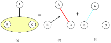
Fig. 1: The entanglement of ${\left|\psi\right\rangle}_{A(BC)}$ ((a) in the figure) consists of two different parts: One is the localizable entanglement onto $AC$ represented by $E_{a}(\rho_{AC})$ ((b) in the figure), and the other part is the unlocalizable entanglement represented by $E_{u}^{\leftarrow}(\rho_{AB})$ ((c) in the figure).

II.2 Properties

II.2.1 Subadditivity

Lemma 2.

For all bipartite states $\rho_{AB}$ and $\sigma_{A^{\prime}B^{\prime}}$,

$$E_{u}^{\leftarrow}(\rho_{AB}\otimes\sigma_{A^{\prime}B^{\prime}})\leq E_{u}^{\leftarrow}(\rho_{AB})+E_{u}^{\leftarrow}(\sigma_{A^{\prime}B^{\prime}}),$$ (10)

where

$$\begin{split}E_{u}^{\leftarrow}(\rho_{AB}\otimes\sigma_{A^{\prime}B^{\prime}})=\min_{\{L_{z}\}}\left[S(\rho_{A}\otimes\sigma_{A^{\prime}})-\sum_{z}r_{z}S(\tau^{z}_{AA^{\prime}})\right],\\ \end{split}$$ (11)

with $r_{z}=\mbox{$\mathrm{tr}$}[(I_{AA^{\prime}}\otimes L_{z})\rho_{AB}\otimes\sigma_{A^{\prime}B^{\prime}}]$, $\tau^{z}_{AA^{\prime}}=\mbox{$\mathrm{tr}$}_{BB^{\prime}}[(I_{AA^{\prime}}\otimes L_{z})\rho_{AB}\otimes\sigma_{A^{\prime}B^{\prime}}]/r_{z}$, and the minimum is taken over all possible rank-1 measurements $\{L_{z}\}$ applied on subsystem $BB^{\prime}$.

Proof.

Let $\{M_{x}\}$ and $\{N_{y}\}$ be the optimal rank-1 measurements on subsystems $B$ and $B^{\prime}$ for $E_{u}^{\leftarrow}(\rho_{AB})$ and $E_{u}^{\leftarrow}(\sigma_{A^{\prime}B^{\prime}})$ respectively, then, we have

$$E_{u}^{\leftarrow} (\rho_{AB})+E_{u}^{\leftarrow}(\sigma_{A^{\prime}B^{\prime}})$$

$$=S(\rho_{A})+S(\sigma_{A^{\prime}})-\sum_{x}p_{x}S(\rho^{x}_{A})-\sum_{y}q_{y}S(\sigma^{y}_{A^{\prime}})$$

$$=S(\rho_{A}\otimes\sigma_{A^{\prime}})-\sum_{xy}p_{x}q_{y}S(\rho^{x}_{A}\otimes\sigma^{y}_{A^{\prime}})$$

$$\geq E_{u}^{\leftarrow}(\rho_{AB}\otimes\sigma_{A^{\prime}B^{\prime}}),$$ (12)

where $p_{x}\rho^{x}_{A}=\mbox{$\mathrm{tr}$}_{B}[(I_{A}\otimes M_{x})\rho_{AB}]$, $q_{y}\sigma^{y}_{A^{\prime}}=\mbox{$\mathrm{tr}$}_{B^{\prime}}[(I_{A^{\prime}}\otimes N_{y})\sigma_{A^{\prime}B^{\prime}}]$, and the second equality is due to the additivity of von Neumann entropy and the definition of $E_{u}^{\leftarrow}(\rho_{AB}\otimes\sigma_{A^{\prime}B^{\prime}})$. ∎

By Lemma 2, we can assure the existence of the regularized UE

$$E_{u,\infty}^{\leftarrow}(\rho_{AB}):=\lim_{n\rightarrow\infty}\frac{E_{u}^{\leftarrow}(\rho_{AB}^{\otimes n})}{n},$$ (13)

which satisfies

$$E_{u,\infty}^{\leftarrow}(\rho_{AB})\leq E_{u}^{\leftarrow}(\rho_{AB}).$$ (14)

II.2.2 Simple Lower Bound

Lemma 3.

For any bipartite state $\rho_{AB}$,

$$E_{u}^{\leftarrow}(\rho_{AB})\geq\max\{I_{c}^{\leftarrow}(\rho_{AB}),~{}0\},$$ (15)

where $I_{c}^{\leftarrow}(\rho_{AB}):=S(\rho_{A})-S(\rho_{AB})$ is the coherent information of $\rho_{AB}$.

Proof.

Let ${\left|\psi\right\rangle}_{ABC}$ be a purification of $\rho_{AB}$, then due to the monotonicity of entanglement, we have

$$E_{a}(\rho_{AC})\leq\min\{S(\rho_{A}),~{}S(\rho_{C})\},$$ (16)

where $\rho_{AC}=\mbox{$\mathrm{tr}$}_{B}{\left|\psi\right\rangle}_{ABC}{\left\langle\psi\right|}$.

Thus, together with Lemma 1, we have

$$E_{u}^{\leftarrow}(\rho_{AB}) =S(\rho_{A})-E_{a}(\rho_{AC})$$

$$\geq\max\{S(\rho_{A})-S(\rho_{C}),~{}0\}$$

$$=\max\{I_{c}^{\leftarrow}(\rho_{AB}),~{}0\},$$ (17)

where the last equality is due to the purity of ${\left|\psi\right\rangle}_{ABC}$, that is, $S(\rho_{C})=S(\rho_{AB})$. ∎

Since ${\left|\psi\right\rangle}_{ABC}^{\otimes n}$ is a purification of both $\rho_{AB}^{\otimes n}$ and $\rho_{BC}^{\otimes n}$, we have

$$E_{u}^{\leftarrow}\left(\rho_{AB}^{\otimes n}\right)+E_{a}\left(\rho_{AC}^{\otimes n}\right)=nS(\rho_{A}).$$ (18)

By taking the limit $n\to\infty$, and due to the relation Smolin-Ver-Win

$$\lim_{n\to\infty}\frac{E_{a}\left(\rho_{AC}^{\otimes n}\right)}{n}=\min\{S(\rho_{A}),S(\rho_{C})\},$$ (19)

we have that

$${E_{u,\infty}^{\leftarrow}}(\rho_{AB})=\max\{I_{c}^{\leftarrow}(\rho_{AB}),0\}.$$ (20)

Eq. (20) implies that, in the asymptotic limit of many copies, separable states do not exhibit quantumness in their correlations, or their correlations are completely erasable. This is a strong evidence that the distinction between separable and entangled states is operational only in asymptotic sense, since separable states can exhibit non-zero UE in finite case.

III Polygamy of entanglement in tripartite quantum systems

For any bipartite pure state ${\left|\phi\right\rangle}_{AB}$, its concurrence, $\mathcal{C}({\left|\phi\right\rangle}_{AB})$ is defined as ww

$$\mathcal{C}({\left|\phi\right\rangle}_{AB})=\sqrt{2(1-\mbox{$\mathrm{tr}$}\rho^{2}_{A})},$$ (21)

where $\rho_{A}=\mbox{$\mathrm{tr}$}_{B}({\left|\phi\right\rangle}_{AB}{\left\langle\phi\right|})$. For any mixed state $\rho_{AB}$, its concurrence is defined via convex-roof extension, that is,

$$\mathcal{C}(\rho_{AB})=\min\sum_{k}p_{k}\mathcal{C}({{\left|\phi_{k}\right\rangle}}_{AB}),$$ (22)

where the minimum is taken over all possible pure state decompositions, $\rho_{AB}=\sum_{k}p_{k}{{\left|\phi_{k}\right\rangle}}_{AB}{\left\langle\phi\right|}_{k}$.

As a dual value to concurrence, CoA lve of $\rho_{AB}$ is defined as

$$\mathcal{C}^{a}(\rho_{AB})=\max\sum_{k}p_{k}\mathcal{C}({{\left|\phi_{k}\right\rangle}}_{AB}),$$ (23)

where the maximum is taken over all possible pure state decompositions of $\rho_{AB}$.

By using concurrence and CoA as the quantification of bipartite entanglement, it was shown that there exists a polygamy relation of entanglement in multi-qubit systems gbs . More precisely, for any pure state ${\left|\psi\right\rangle}_{A_{1}\cdots A_{n}}$ in an $n$-qubit system $\mathcal{H}_{A_{1}}\otimes\cdots\otimes\mathcal{H}_{A_{n}}$ where $\mathcal{H}_{A_{i}}\cong\mathbb{C}^{2}$ for $i=1,\ldots,n$,

$$\mathcal{C}_{A_{1}(A_{2}\cdots A_{n})}^{2}\leq(\mathcal{C}^{a}_{A_{1}A_{2}})^{2}+\cdots+(\mathcal{C}^{a}_{A_{1}A_{n}})^{2},$$ (24)

where $\mathcal{C}_{A_{1}(A_{2}\cdots A_{n})}$ is the concurrence of ${\left|\psi\right\rangle}_{A_{1}\cdots A_{n}}$ with respect to the bipartite cut $A_{1}$ and $A_{2}\cdots A_{n}$, and $\mathcal{C}^{a}_{A_{1}A_{i}}$ is the CoA of $\rho_{A_{1}A_{i}}=\mbox{$\mathrm{tr}$}_{A_{2}\cdots A_{i-1}A_{i+1}\cdots A_{n}}\left({\left|\psi\right\rangle}_{A_{1}\cdots A_{n}}{\left\langle\psi\right|}\right)$ for $i=2,\ldots,n$.

In this section, we provide an analytic upper bound of UE in Eq. (8), and derive a polygamy inequality of entanglement in terms of von-Neumann entropy and EoA for tripartite quantum systems of arbitrary dimension.

First, for an upper bound of UE, we have the following theorem.

Theorem 4.

For any bipartite state $\rho_{AB}$ in a bipartite quantum system $\mathcal{H}_{A}\otimes\mathcal{H}_{B}$,

$$E_{u}^{\leftarrow}(\rho_{AB})\leq\frac{I(\rho_{AB})}{2},$$ (25)

where $I(\rho_{AB})=S(\rho_{A})+S(\rho_{B})-S(\rho_{AB})$ is the mutual information of $\rho_{AB}$.

Proof.

Let $\rho_{B}=\sum_{i=0}^{d_{B}-1}\lambda_{i}{\left|e_{i}\right\rangle}_{B}{\left\langle e_{i}\right|}$ be a spectral decomposition of $\rho_{B}=\mbox{$\mathrm{tr}$}_{A}(\rho_{AB})$ where $d_{B}$ is the dimension of the subsystem $\mathcal{H}_{B}$. The proof method follows the construction used in christandl .

For any state $\sigma\in\mathcal{H}_{B}$, define the channels

$$M_{0}(\sigma): =\sum_{i=0}^{d_{B}-1}{\left|e_{i}\right\rangle}{\left\langle e_{i}\right|}\sigma{\left|e_{i}\right\rangle}{\left\langle e_{i}\right|}$$

$$M_{1}(\sigma): =\sum_{i=0}^{d_{B}-1}|\tilde{e}_{j}\rangle\langle\tilde{e}_{j}|\sigma|\tilde{e}_{j}\rangle\langle\tilde{e}_{j}|,$$ (26)

where $\{|\tilde{e}_{j}\rangle\}_{j}$ is the Fourier basis such that,

$$|\tilde{e}_{j}\rangle=\frac{1}{\sqrt{d}}\sum_{k=0}^{d_{B}-1}\omega_{d}^{jk}{\left|e_{k}\right\rangle},~{}j=0,\ldots,d_{B}-1,$$ (27)

and $\omega_{d}=e^{\frac{2\pi i}{d}}$ is the $d$-th root of unity.

Notice that $M_{0}(\rho_{B})=\rho_{B}$, and $M_{1}(\rho_{B})=\frac{1}{d_{B}}I_{B}$, so that $M_{1}(M_{0}(\rho_{B}))=M_{0}(M_{1}(\rho_{B}))=\frac{1}{d_{B}}I_{B}$. We can also write

$$M_{0}(\sigma)=\frac{1}{d_{B}}\sum_{b=0}^{d_{B}-1}Z^{b}\sigma Z^{-b},~{}M_{1}(\sigma)=\frac{1}{d_{B}}\sum_{a=0}^{d_{B}-1}X^{a}\sigma X^{-a},$$ (28)

where $Z$ and $X$ are generalized $d_{B}$-dimensional Pauli operators,

$$Z= \sum_{j=0}^{d_{B}-1}\omega_{d}^{j}{\left|e_{j}\right\rangle}{\left\langle e_{j}\right|},$$

$$X= \sum_{j=0}^{d_{B}-1}{\left|e_{j+1}\right\rangle}{\left\langle e_{j}\right|}=\sum_{j=0}^{d_{B}-1}\omega_{d}^{-j}|\tilde{e}_{j}\rangle\langle\tilde{e}_{j}|.$$ (29)

In the following, we will write

$$(I_{A}\otimes M_{0})(\rho_{AB}) =\sum_{i=0}^{d_{B}-1}\sigma_{A}^{i}\otimes\lambda_{i}{\left|e_{i}\right\rangle}_{B}{\left\langle e_{i}\right|},$$

$$(I_{A}\otimes M_{1})(\rho_{AB}) =\sum_{j=0}^{d_{B}-1}\tau_{A}^{j}\otimes\frac{1}{d_{B}}|\tilde{e}_{j}\rangle_{B}\langle\tilde{e}_{j}|,$$ (30)

where $\lambda_{i}\sigma_{A}^{i}=\mbox{$\mathrm{tr}$}_{B}[(I_{A}\otimes{\left|e_{i}\right\rangle}_{B}{\left\langle e_{i}\right|})\rho_{AB}]$, and $\tau_{A}^{j}/d_{B}=\mbox{$\mathrm{tr}$}_{B}[(I_{A}\otimes|\tilde{e}_{j}\rangle_{B}\langle\tilde{e}_{j}|)\rho_{AB}]$ for $i,~{}j\in\{0,\cdots,d_{B}-1\}$.

The induced ensembles on $A$ by the channels $M_{0}$ and $M_{1}$ will be denoted by $\mathcal{E}_{0}:=\{\lambda_{i},\sigma_{A}^{i}\}_{i}$ and $\mathcal{E}_{1}:=\{\frac{1}{d_{B}},\tau_{A}^{j}\}_{j}$, and the entropy defects of the induced ensembles on $A$ will be denoted as

$$\chi(\mathcal{E}_{0})= S(\rho_{A})-\sum_{i=0}^{d_{B}-1}\lambda_{i}S(\sigma_{A}^{i}),$$

$$\chi(\mathcal{E}_{1})= S(\rho_{A})-\frac{1}{d_{B}}\sum_{i=0}^{d_{B}-1}S(\tau_{A}^{j}).$$ (31)

By defining a four-partite quantum state $\Omega_{XYAB}$ in $\mathcal{B}\left(\mbox{$\mathbb{C}$}^{d_{B}}\otimes\mbox{$\mathbb{C}$}^{d_{B}}\otimes\mbox{$\mathbb{C}$}^{d_{A}}\otimes\mbox{$\mathbb{C}$}^{d_{B}}\right)$ such that

$$\Omega_{XYAB}:=\frac{1}{d^{2}_{B}}\sum_{x,y=0}^{d_{B}-1}{\left|x\right\rangle}_{X}{\left\langle x\right|}\otimes{\left|y\right\rangle}_{Y}{\left\langle y\right|}\otimes(I_{A}\otimes X^{x}_{B}Z^{y}_{B})\rho_{AB}(I_{A}\otimes Z^{-y}_{B}X^{-x}_{B}),$$ (32)

we have

$$\Omega_{XAB}= \frac{1}{d_{B}}\sum_{x=0}^{d_{B}-1}{\left|x\right\rangle}_{X}{\left\langle x\right|}\otimes X^{x}_{B}\left(\sum_{i=0}^{d_{B}-1}\sigma_{A}^{i}\otimes\lambda_{i}{\left|e_{i}\right\rangle}_{B}{\left\langle e_{i}\right|}\right)X_{B}^{-x},$$

$$\Omega_{YAB}= \frac{1}{d_{B}}\sum_{y=0}^{d_{B}-1}{\left|y\right\rangle}_{Y}{\left\langle y\right|}\otimes Z_{B}^{y}\left(\sum_{j=0}^{d_{B}-1}\tau_{A}^{j}\otimes\frac{1}{d_{B}}|\tilde{e}_{j}\rangle_{B}\langle\tilde{e}_{j}|\right)Z_{B}^{-y},$$ (33)

and

$$\Omega_{AB}=\rho_{A}\otimes\frac{I_{B}}{d_{B}}.$$ (34)

By straightforward calculation, we can obtain

$$I(\Omega_{X(AB)})= S(\Omega_{X})+S(\Omega_{AB})-S(\Omega_{XAB})$$

$$= \log d_{B}+\log d_{B}+S(\rho_{A})-\log d_{B}$$

$$~{}~{}~{}~{}~{}~{}~{}~{}~{}~{}~{}~{}-S\left(\sum_{i}\sigma_{A}^{i}\otimes\lambda_{i}{\left|e_{i}\right\rangle}_{B}{\left\langle e_{i}\right|}\right)$$

$$= \log d_{B}+S(\rho_{A})-H(\vec{\lambda})-\sum_{i}\lambda_{i}S(\sigma_{A}^{i})$$

$$= \log d_{B}-S(\rho_{B})+\chi(\mathcal{E}_{0}),$$ (35)

where $I(\Omega_{X(AB)})$ is the mutual information of $\Omega_{X(AB)}$ with respect to the bipartite cut $X-AB$, and the second, third equalities are due to the joint entropy theorem nc . Analogously, we have

$$I(\Omega_{Y(AB)})=\chi(\mathcal{E}_{1}),$$

$$I(\Omega_{(XY)(AB)})=\log d_{B}+S(\rho_{A})-S(\rho_{AB})$$

$$~{}~{}~{}~{}~{}~{}~{}~{}~{}~{}~{}~{}~{}~{}~{}~{}~{}~{}=\log d_{B}+I_{c}^{\leftarrow}(\rho_{AB}).$$ (36)

Due to the independence of subsystems $X$ and $Y$, we have $I(\Omega_{(XY)(AB)})\geq I(\Omega_{X(AB)})+I(\Omega_{Y(AB)})$, which implies

$$\chi(\mathcal{E}_{0})+\chi(\mathcal{E}_{1})\leq I(\rho_{AB}).$$ (37)

Since $\chi(\mathcal{E}_{0})$ and $\chi(\mathcal{E}_{1})$ of Eq. (37) can be obtained, respectively, from $\rho_{AB}$ by rank-1 measurements $\{{\left|e_{i}\right\rangle}_{B}{\left\langle e_{i}\right|}\}_{i}$ and $\{|\tilde{e}_{j}\rangle_{B}\langle\tilde{e}_{j}|\}_{j}$ of subsystem $B$, by defining a rank-1 measurement

$$\left\{\frac{{\left|e_{i}\right\rangle}_{B}{\left\langle e_{i}\right|}}{2},\frac{|\tilde{e}_{j}\rangle_{B}\langle\tilde{e}_{j}|}{2}\right\}_{i,j},$$ (38)

we have

$$E_{u}^{\leftarrow}(\rho_{AB})\leq\frac{\chi(\mathcal{E}_{0})}{2}+\frac{\chi(\mathcal{E}_{1})}{2}\leq\frac{I(\rho_{AB})}{2},$$ (39)

which completes the proof. ∎

Corollary 1.

For any tripartite pure state ${\left|\psi\right\rangle}_{ABC}$, we have

$$S(\rho_{A})\leq E_{a}(\rho_{AB})+E_{a}(\rho_{AC}).$$ (40)

Proof.

By Lemma 7, we have

$$E_{a}(\rho_{AC}) =S(\rho_{A})-E_{u}^{\leftarrow}(\rho_{AB}),$$

$$E_{a}(\rho_{AB}) =S(\rho_{A})-E_{u}^{\leftarrow}(\rho_{AC}),$$ (41)

and thus,

$$E_{a}(\rho_{AC})+E_{a}(\rho_{AB})=2S(\rho_{A})-E_{u}^{\leftarrow}(\rho_{AB})-E_{u}^{\leftarrow}(\rho_{AC}).$$ (42)

Now, by Theorem 4, we have

$$E_{a}(\rho_{AC})+ E_{a}(\rho_{AB})$$

$$\geq 2S(\rho_{A})-\frac{I(\rho_{AB})}{2}-\frac{I(\rho_{AC})}{2}$$

$$= 2S(\rho_{A})-S(\rho_{A})/2-S(\rho_{B})/2+S(\rho_{AB})/2$$

$$-S(\rho_{A})/2-S(\rho_{C})/2+S(\rho_{AC})/2$$

$$= S(\rho_{A}).$$ (43)

∎

Corollary 40 tells us that for a tripartite pure state of arbitrary dimension, there exists a polygamy relation of entanglement in terms of entropy of entanglement and EoA. Furthermore, this is, we believe, the first result of the polygamous (or dually monogamous) property of distribution of entanglement in multipartite higher-dimensional quantum systems rather than qubits.

IV Polygamy relation of entanglement in multi-qubit quantum systems

In this section, we show that the polygamy inequality of entanglement in Corollary 40 can be generalized into multipartite quantum systems for the case when each subsystem is a two-level quantum system. By investigating the functional relation between concurrence and EoF in two-qubit systems ww , we show that there exists a polygamy inequality of entanglement in terms of entropy and EoA in $n$-qubit systems. We also show that, in three-qubit systems, we have a more tight polygamy inequality than Eq. (40) in Corollary 40.

First, let us consider the functional relation of concurrence with EoF in two-qubit systems. For a 2-qubit mixed state $\rho_{AB}$ (or a pure state ${\left|\psi\right\rangle}_{AB}\in\mathbb{C}^{2}\otimes\mathbb{C}^{d}$), the relation between its concurrence, $\mathcal{C}_{AB}$ and $E_{f}(\rho_{AB})$ can be given as a monotone increasing, convex function $\mathcal{E}$ ww , such that

$$E_{f}(\rho_{AB})={\mathcal{E}}(\mathcal{C}_{AB}),$$ (44)

where

$${\mathcal{E}}(x)=H\Bigl{(}{1\over 2}+{1\over 2}\sqrt{1-x^{2}}\Bigr{)},\hskip 14.22636pt\mbox{for }0\leq x\leq 1,$$ (45)

and $H(\cdot)$ is the binary entropy function $H(x)=-[x\log_{2}x+(1-x)\log_{2}(1-x)]$. The same function $\mathcal{E}(x)$ relates also the EoA of a bipartite state $\rho_{AB}$ with its CoA via the equation

$$E_{a}(\rho_{AB})\geq\mathcal{E}(\mathcal{C}_{AB}^{a}),$$ (46)

which is due to the convexity of ${\mathcal{E}}$ and the definition of EoA. The following lemma shows an important property of the function $\mathcal{E}(x)$.

Lemma 5.

$${\mathcal{E}}(\sqrt{x^{2}+y^{2}})\leq{\mathcal{E}}(x)+{\mathcal{E}}(y),$$ (47)

for $0\leq x,~{}y\leq 1$ such that $0\leq x^{2}+y^{2}\leq 1$.

Proof.

By considering

$$f(x,y)={\mathcal{E}}(x)+{\mathcal{E}}(y)-{\mathcal{E}}(\sqrt{x^{2}+y^{2}}),$$ (48)

as a two-vairable real-valued function on the domain $D=\{(x,y)|0\leq x,~{}y\leq 1,0\leq\ x^{2}+y^{2}\leq 1\}$, it is enough to show that $f(x,y)\geq 0$ in $D$.

Since $D$ is a compact subset in $\mbox{$\mathbb{R}$}^{2}$, whereas $f$ is analytic on the interior of $D$, and continuous on $D$, the minimum value of $f$ arises only on the critical points or on the boundary of $D$. It can be directly checked that $f$ does not have any vanishing gradient on the interior of $D$, and has non-negative function values on the boundary of $D$. Thus, $f$ is non-negative on the domain $D$. ∎

IV.1 Three-qubit systems

A direct observation from CKW shows that, for a 3-qubit pure state ${\left|\psi\right\rangle}_{ABC}$,

$$\mathcal{C}_{A(BC)}^{2}=\mathcal{C}_{AB}^{2}+({\mathcal{C}^{a}_{AC}})^{2},$$ (49)

where $\mathcal{C}_{AB}$ and $\mathcal{C}^{a}_{AC}$ are the concurrence and concurrence of assistance of $\rho_{AB}$ and $\rho_{AC}$ respectively. (Later, Eq. (49) was formally shown in ys .) From Eq. (49) together with Lemma 5, we have the following theorem.

Theorem 6.

For a three-qubit pure state ${\left|\psi\right\rangle}_{ABC}$,

$$S(\rho_{A})\leq E_{f}(\rho_{AB})+E_{a}(\rho_{AC}).$$ (50)

Proof.

Since ${\left|\psi\right\rangle}_{ABC}$ is a bipartite pure state in $\mathbb{C}^{2}\otimes\mathbb{C}^{4}$ with respect to the bipartite cut $A$ and $BC$, we have,

$$S(\rho_{A})=E_{f}(\psi_{A(BC)})={\mathcal{E}}(\mathcal{C}_{A(BC)}).$$ (51)

Thus,

$$S(\rho_{A}) = {\mathcal{E}}(\mathcal{C}_{A(BC)})$$ (52)

$$= {\mathcal{E}}(\sqrt{\mathcal{C}^{2}_{AB}+{\mathcal{C}^{a}_{AC}}^{2}}~{})$$

$$\leq {\mathcal{E}}(\mathcal{C}_{AB})+{\mathcal{E}}(\mathcal{C}^{a}_{AC})$$

$$\leq E_{f}(\rho_{AB})+E_{a}(\rho_{AC}),$$

where the first inequality is by Lemma 5, and the second inequality is by Eq. (46). ∎

Thus, the polygamy relation of distributed entanglement in tripartite quantum systems obtained in Corollary 40 can have a more tight form in three-qubit systems. Furthermore, the result of Theorem 50 together with Eqs. (3) and (7) give us the following corollary.

Corollary 2.

For any two-qubit mixed state $\rho_{AB}$ with rank less than or equal to two,

$$I^{\leftarrow}(\rho_{AB})\leq E_{a}(\rho_{AB}),$$ (53)

$$E_{u}^{\leftarrow}(\rho_{AB})\leq E_{f}(\rho_{AB}).$$ (54)

Remark 1.

Eq. (54) of Corollary 54 implies that any two-qubit separable state $\rho_{AB}$ of rank less than or equal to two has zero UE, $E_{u}^{\leftarrow}(\rho_{AB})=0$. However, this is not generally true for two-qubit separable states of rank larger than two. Here, we provide an example of two-qubit rank-three separable state with non-zero UE.

Example: Let us consider the following state in $\mbox{$\mathbb{C}$}^{2}\otimes\mbox{$\mathbb{C}$}^{2}\otimes\mbox{$\mathbb{C}$}^{3}$ quantum system CCJKKL ,

$${\left|\Psi\right\rangle}_{ABC}=\frac{1}{\sqrt{2}}{\left|x\right\rangle}_{AC}{\left|0\right\rangle}_{B}+\frac{1}{\sqrt{2}}{\left|y\right\rangle}_{AC}{\left|1\right\rangle}_{B},$$ (55)

where ${\left|x\right\rangle}$ and ${\left|y\right\rangle}$ are two orthogonal states in the $\mbox{$\mathbb{C}$}^{2}\otimes\mbox{$\mathbb{C}$}^{3}$ such that

$${\left|x\right\rangle}= ({\left|02\right\rangle}+\sqrt{2}{\left|10\right\rangle})/{\sqrt{3}},$$

$${\left|y\right\rangle}= ({\left|12\right\rangle}+\sqrt{2}{\left|01\right\rangle})/{\sqrt{3}}.$$ (56)

First, since $\rho_{A}=({\left|0\right\rangle}_{A}{\left\langle 0\right|}+{\left|1\right\rangle}_{A}{\left\langle 1\right|})/2$, it is clear that $\mathcal{C}_{A(BC)}=\sqrt{2(1-\mbox{$\mathrm{tr}$}\rho^{2}_{A})}=1$, therefore we have $S(\rho_{A})=1$.

Since $\rho_{AC}=({\left|x\right\rangle}_{AC}{\left\langle x\right|}+{\left|y\right\rangle}_{AC}{\left\langle y\right|})/2$, Hughston-Jozsa-Wootters (HJW) theorem HJW says that for any decompositions of $\rho_{AC}=\sum_{i}p_{i}{\left|\phi_{i}\right\rangle}_{AC}{\left\langle\phi_{i}\right|}$, there exists an unitary operator $(u_{ij})$ such that $\sqrt{p_{i}}{\left|\phi_{i}\right\rangle}_{AC}=(u_{i1}{\left|x\right\rangle}_{AC}+u_{i2}{\left|y\right\rangle}_{AC})/\sqrt{2}$ with $2p_{i}=|u_{i1}|^{2}+|u_{i2}|^{2}$. Thus,

$$\mbox{$\mathrm{tr}$}_{C}({\left|\phi_{i}\right\rangle}_{AC}{\left\langle\phi_{i}\right|})= \frac{1}{6p_{i}}\begin{pmatrix}|u_{i1}|^{2}+2|u_{i2}|^{2}&u_{i1}u_{i2}^{*}\\ u_{i2}u_{i1}^{*}&|u_{i2}|^{2}+2|u_{i1}|^{2}\end{pmatrix}$$

$$= \frac{1}{3}I_{A}+\frac{1}{3}{\left|\psi_{i}\right\rangle}_{A}{\left\langle\psi_{i}\right|},$$ (57)

with ${\left|\psi_{i}\right\rangle}=(u_{i2}^{*}{\left|0\right\rangle}+u_{i1}^{*}{\left|1\right\rangle})/{\sqrt{2p_{i}}}$, and we obtain that $\mathcal{C}({\left|\phi_{i}\right\rangle}_{AC})=\frac{2\sqrt{2}}{3}$ for any pure state ${\left|\phi_{i}\right\rangle}_{AC}$ in any pure state decomposition of $\rho_{AC}$.

Since ${\left|\phi_{i}\right\rangle}_{AC}$ is a $2\otimes 3$ pure state, we have

$$E_{f}({\left|\phi_{i}\right\rangle}_{AC}) = {\mathcal{E}}(\mathcal{C}({\left|\phi_{i}\right\rangle}_{AC}))$$ (58)

$$= H\Bigl{(}\frac{2}{3}\Bigr{)}$$

$$= \log_{2}3-\frac{2}{3},$$

and thus $E_{f}(\rho_{AC})=E_{a}(\rho_{AC})=\log_{2}3-\frac{2}{3}$.

Now, we have $E_{u}^{\leftarrow}(\rho_{AB})=S(\rho_{A})-E_{a}(\rho_{AC})=\frac{5}{3}-\log_{2}3>0$, whereas, it can be easily seen that $\rho_{AB}$ has a Positive Partial Transposition (PPT) which is equivalent to separability for two-qubit states horo1 . Thus, $\rho_{AB}$ is a two-qubit, rank-three separable state with non-zero UE.

IV.2 $n$-qubit systems

The polygamy inequality of entanglement in $n$-qubit systems in Eq. (24) gives us an inequality

$$\mathcal{C}_{A_{1}(A_{2}\cdots A_{n})}\leq\sqrt{(\mathcal{C}^{a}_{A_{1}A_{2}})^{2}+\cdots+(\mathcal{C}^{a}_{A_{1}A_{n}})^{2}}.$$ (59)

Thus, together with Lemma 5, we have the following theorem.

Theorem 7.

For any $n$-qubit pure state ${\left|\psi\right\rangle}_{A_{1}\cdots A_{n}}$,

$$S(\rho_{A_{1}})\leq E_{a}(\rho_{A_{1}A_{2}})+\cdots+E_{a}(\rho_{A_{1}A_{n}}).$$ (60)

Proof.

First, let us assume that $(\mathcal{C}^{a}_{A_{1}A_{2}})^{2}+\cdots+(\mathcal{C}^{a}_{A_{1}A_{n}})^{2}\leq 1$, then we have

$$S(\rho_{A_{1}})= {\mathcal{E}}(\mathcal{C}_{A_{1}(A_{2}\cdots A_{n})})$$

$$\leq {\mathcal{E}}\left(\sqrt{(\mathcal{C}^{a}_{A_{1}A_{2}})^{2}+\cdots+(\mathcal{C}^{a}_{A_{1}A_{n}})^{2}}\right)$$

$$\leq {\mathcal{E}}\left(\mathcal{C}^{a}_{A_{1}A_{2}}\right)+{\mathcal{E}}\left(\sqrt{(\mathcal{C}^{a}_{A_{1}A_{3}})^{2}+\cdots+(\mathcal{C}^{a}_{A_{1}A_{n}})^{2}}\right)$$

$$\leq {\mathcal{E}}\left(\mathcal{C}^{a}_{A_{1}A_{2}}\right)+{\mathcal{E}}\left(\mathcal{C}^{a}_{A_{1}A_{3}}\right)+\cdots+{\mathcal{E}}\left(\mathcal{C}^{a}_{A_{1}A_{n}}\right)$$

$$\leq E_{a}\left(\rho_{A_{1}A_{2}}\right)+\cdots+E_{a}\left(\rho_{A_{1}A_{n}}\right),$$ (61)

where the first inequality is due to the monotonicity of the function $\mathcal{E}$, the second and third inequalities are obtained by iterating Lemma 5, and the last inequality is by Eq. (46).

Now, assume that $(\mathcal{C}^{a}_{A_{1}A_{2}})^{2}+\cdots+(\mathcal{C}^{a}_{A_{1}A_{n}})^{2}>1$. Since $S(\rho_{A_{1}})\leq 1$ for any $n$-qubit pure state ${\left|\psi\right\rangle}_{A_{1}\cdots A_{n}}$, it is enough to show that $E_{a}(\rho_{A_{1}A_{2}})+\cdots+E_{a}(\rho_{A_{1}A_{n}})\geq 1$.

Let us first note that there exist $k\in\{2,\ldots,n-1\}$ that satisfies

$$(\mathcal{C}^{a}_{A_{1}A_{2}})^{2}+\cdots+(\mathcal{C}^{a}_{A_{1}A_{k}})^{2}\leq 1,$$

$$(\mathcal{C}^{a}_{A_{1}A_{2}})^{2}+\cdots+(\mathcal{C}^{a}_{A_{1}A_{k+1}})^{2}>1,$$ (62)

and let

$$T=(\mathcal{C}^{a}_{A_{1}A_{2}})^{2}+\cdots+(\mathcal{C}^{a}_{A_{1}A_{k+1}})^{2}-1.$$ (63)

Since, $(\mathcal{C}^{a}_{A_{1}A_{k+1}})^{2}-T=1-(\mathcal{C}^{a}_{A_{1}A_{2}})^{2}-\cdots-(\mathcal{C}^{a}_{A_{1}A_{k}})^{2}$, we have

$$0\leq(\mathcal{C}^{a}_{A_{1}A_{k+1}})^{2}-T\leq 1,$$ (64)

and

$$1= \mathcal{E}\left(\sqrt{(\mathcal{C}^{a}_{A_{1}A_{2}})^{2}+\cdots+(\mathcal{C}^{a}_{A_{1}A_{k+1}})^{2}-T}\right)$$

$$\leq \mathcal{E}\left(\sqrt{(\mathcal{C}^{a}_{A_{1}A_{2}})^{2}+\cdots+(\mathcal{C}^{a}_{A_{1}A_{k}})^{2}}\right)$$

$$~{}~{}~{}~{}~{}~{}~{}~{}~{}~{}~{}~{}~{}~{}~{}~{}+\mathcal{E}\left(\sqrt{\left(\mathcal{C}^{a}_{A_{1}A_{k+1}}\right)^{2}-T}\right)$$

$$\leq \mathcal{E}\left(\mathcal{C}^{a}_{A_{1}A_{2}}\right)+\cdots+\mathcal{E}\left(\mathcal{C}^{a}_{A_{1}A_{k}}\right)+\mathcal{E}\left(\mathcal{C}^{a}_{A_{1}A_{k+1}}\right)$$

$$\leq E_{a}(\rho_{A_{1}A_{2}})+\cdots+E_{a}(\rho_{A_{1}A_{n}}),$$ (65)

where the first and second inequalities are by Lemma 5 and by monotonicity of $\mathcal{E}$, and the last inequality is by Eq. (46). ∎

V Unlocalizable Entanglement versus Other Measures of Correlation

In this section, we provide some properties of UE concerned with several other correlation measures. By investigating the relation between UE and EoF in $2\otimes 2\otimes d$ quantum system, we show that any two-qubit state with zero UE is a separable state. We also provide a quantitative relation among entropy, localizable entanglement, and UE for tripartite mixed states.

V.1 $2\otimes 2\otimes d$ pure state

Let ${\left|\psi\right\rangle}_{ABC}$ be a tripartite pure state in $\mathbb{C}^{2}\otimes\mathbb{C}^{2}\otimes\mathbb{C}^{d}$.

Theorem 8.

For any 2-qubit state $\rho_{AB}$,

$$E_{u}^{\leftarrow}(\rho_{AB})=0\Longrightarrow\rho_{AB}\textrm{ separable},$$ (66)

or, equivalently, if $S(\rho_{A})=E_{a}(\rho_{AC})$, then $E_{f}(\rho_{AB})=0$.

Proof.

Suppose $S(\rho_{A})=E_{a}(\rho_{AC})$, and let $\rho_{AC}=\sum_{i}p_{i}{\left|\phi^{i}\right\rangle}_{AC}{\left\langle\phi^{i}\right|}$ be an optimal decomposition such that,

$$E_{a}(\rho_{AC}) = \sum_{i}p_{i}E({\left|\phi^{i}\right\rangle}_{AC})$$ (67)

$$= \sum_{i}p_{i}S(\rho^{i}_{A}),$$

where $\rho^{i}_{A}=\mbox{$\mathrm{tr}$}_{C}({\left|\phi^{i}\right\rangle}_{AC}{\left\langle\phi^{i}\right|})$ and $\rho_{A}=\sum_{i}p_{i}\rho^{i}_{A}$.

The concavity of von Neumann entropy says, $S(\rho_{A})\geq\sum_{i}p_{i}S(\rho^{i}_{A})$ and the equality holds if and only if $\rho^{i}_{A}$ are identical for all $i$. So, by the assumption, $\rho^{i}_{A}$ are identical for all $i$.

Since ${\left|\phi^{i}\right\rangle}_{AC}$ is a pure state in $2\otimes d$ system and its concurrence is $\mathcal{C}({\left|\phi^{i}\right\rangle}_{AC})=2\sqrt{det\rho^{i}_{A}}$, we also have that $\mathcal{C}({\left|\phi^{i}\right\rangle}_{AC})$ are identical for all $i$, say $\mathcal{C}({\left|\phi^{i}\right\rangle}_{AC})=\mathcal{C}^{*}_{AC}$.

Now, we have

$$S(\rho^{i}_{A})=E_{f}({\left|\phi^{i}\right\rangle}_{AC})=\mathcal{E}(\mathcal{C}({\left|\phi^{i}\right\rangle}_{AC}))=\mathcal{E}(\mathcal{C}^{*}_{AC}),$$ (68)

for all $i$, and

$$\mathcal{E}(\mathcal{C}_{A(BC)}) = E_{f}({\left|\psi_{A(BC)}\right\rangle})$$ (69)

$$= S(\rho_{A})$$

$$= \sum_{i}p_{i}S(\rho^{i}_{A})$$

$$= \sum_{i}p_{i}\mathcal{E}(\mathcal{C}({\left|\phi^{i}\right\rangle}_{AC}))$$

$$= \mathcal{E}(\mathcal{C}^{*}_{AC}),$$

where $\mathcal{C}_{A(BC)}$ is the concurrence of ${\left|\psi\right\rangle}_{ABC}$ between subsystems $A$ and $BC$, and $\mathcal{E}(\cdot)$ is the function in Eq. (45).

Since $\mathcal{E}(\cdot)$ is strictly monotone increasing, (the first derivative $\frac{d}{d\mathcal{C}}\mathcal{E}(\mathcal{C})$ is 0 at $\mathcal{C}=0$ and positive elsewhere), we have

$$\mathcal{C}_{A(BC)}=\mathcal{C}^{*}_{AC},$$ (70)

therefore

$$\mathcal{C}_{A(BC)}\geq\mathcal{C}^{a}_{AC}\geq\sum_{i}p_{i}\mathcal{C}({\left|\phi^{i}\right\rangle}_{AC})=\mathcal{C}^{*}_{AC}=\mathcal{C}_{A(BC)},$$ (71)

and thus,

$$\mathcal{C}_{A(BC)}=\mathcal{C}^{a}_{AC}.$$ (72)

Now, by the Theorem 3 in CCJKKL , we have $\mathcal{C}(\rho_{AB})=0$ where $\rho_{AB}$ is a 2-qubit state, which implies $E_{f}(\rho_{AB})=0.$ ∎

Any two-qubit state with zero UE is separable by Theorem 8, and any two-qubit separable state with rank less than or equal to two has zero UE by Corollary 54. However, the converse of Theorem 8 is not generally true, since Remark 1 provides us a two-qubit separable state with non-zero UE.

V.2 Tripartite Mixed State

Since it is known that the EoA is not a bipartite measure nor an entanglement monotone gs , it is not clear yet if there is any quantitative relation between $E_{a}(\rho_{AB})$ and $E_{a}(\rho_{A(BD)})$ for a tripartite mixed state $\rho_{ABD}$. In fact, this is equivalent to the quantitative relation between $E_{u}^{\leftarrow}(\rho_{AC})$ and $E_{u}^{\leftarrow}(\rho_{A(CD)})$. This is because, if we consider a purification ${\left|\psi\right\rangle}_{ABCD}$ of $\rho_{ABD}$, then any direction of a quantitative relation between $E_{a}(\rho_{AB})$ and $E_{a}(\rho_{A(BD)})$, say $E_{a}(\rho_{AB})\leq E_{a}(\rho_{A(BD)})$, would give us

$$S(\rho_{A})= E_{u}^{\leftarrow}(\rho_{A(CD))})+E_{a}(\rho_{AB})$$

$$= E_{u}^{\leftarrow}(\rho_{AC)})+E_{a}(\rho_{A(BD)})$$

$$\geq E_{u}^{\leftarrow}(\rho_{AC)})+E_{a}(\rho_{AB}),$$ (73)

which implies $E_{u}^{\leftarrow}(\rho_{AC})\leq E_{u}^{\leftarrow}(\rho_{A(CD)})$.

In this section, we pay our attentions only to local rank-1 measurements of each subsystems, and we derive a quantitative relation between localizable entanglement, and UE for tripartite mixed states.

For $\rho_{ACD}=\mbox{$\mathrm{tr}$}_{B}{\left|\psi\right\rangle}_{ABCD}{\left\langle\psi\right|}$, let us define

$$\begin{split}\widetilde{E}_{u}^{\leftarrow}(\rho_{A(CD)})&=\min_{\{M_{x}\otimes N_{y}\}}\left[S(\rho_{A})-\sum_{x,y}p_{xy}S(\rho^{xy}_{A})\right],\\ \end{split}$$ (74)

where $p_{xy}\equiv\mbox{$\mathrm{tr}$}[(I_{A}\otimes M_{x}\otimes N_{y})\rho_{ACD}]$ is the probability of the outcome $x$ and $y$ on subsystems $C$ and $D$ respectively, and $\rho^{xy}_{A}\equiv\mbox{$\mathrm{tr}$}_{CD}[(I_{A}\otimes M_{x}\otimes N_{y})\rho_{ACD}]/p_{xy}$ is the state of system $A$ when the outcome were $x$ and $y$. The minimum in Eq. (74) is taken over all possible rank-1 measurements $\{M_{x}\}$ and $\{N_{y}\}$ on subsystems $C$ and $D$ respectively. By definition, we have

$$\widetilde{E}_{u}^{\leftarrow}(\rho_{A(CD)})\geq E_{u}^{\leftarrow}(\rho_{A(CD)}).$$ (75)

Furthermore, we have the following lemma.

Lemma 9.

For any tripartite state $\rho_{ACD}$,

$$\widetilde{E}_{u}^{\leftarrow}(\rho_{A(CD)})\geq E_{u}^{\leftarrow}(\rho_{AC}).$$ (76)

Proof.

For $\rho_{ACD}$, let $\{M_{x}\}$ and $\{N_{y}\}$ are the optimal rank-1 measurements of $C$ and $D$ respectively, such that

$$\widetilde{E}_{u}^{\leftarrow}(\rho_{A(CD)})=S(\rho_{A})-\sum_{x,y}p_{xy}S(\rho^{xy}_{A}).$$ (77)

Due to the concavity of von Neumann entropy, we have

$$\widetilde{E}_{u}^{\leftarrow}(\rho_{A(CD)}) =S(\rho_{A})-\sum_{x,y}p_{xy}S(\rho^{xy}_{A})$$

$$=S(\rho_{A})-\sum_{x}p_{x}\left[\sum_{y}\frac{p_{xy}}{p_{x}}S(\rho^{xy}_{A})\right]$$

$$\geq S(\rho_{A})-\sum_{x}p_{x}S\left(\sum_{y}\frac{p_{xy}}{p_{x}}\rho^{xy}_{A}\right)$$

$$=S(\rho_{A})-\sum_{x}p_{x}S(\rho^{x}_{A})$$

$$\geq E_{u}^{\leftarrow}(\rho_{AC}),$$ (78)

where

$$p_{x} =\mbox{$\mathrm{tr}$}_{AC}\left[(I_{A}\otimes M_{x})\rho_{AC}\right]$$

$$=\mbox{$\mathrm{tr}$}_{ACD}\left[(I_{A}\otimes M_{x}\otimes I_{D})\rho_{ACD}\right]$$

$$=\sum_{y}\mbox{$\mathrm{tr}$}_{ACD}\left[(I_{A}\otimes M_{x}\otimes N_{y})\rho_{ACD}\right]$$

$$=\sum_{y}p_{xy},$$ (79)

$$\rho^{x}_{A} =\frac{1}{p_{x}}\mbox{$\mathrm{tr}$}_{C}\left[(I_{A}\otimes M_{x})\rho_{AC}\right]$$

$$=\frac{1}{p_{x}}\mbox{$\mathrm{tr}$}_{CD}\left[(I_{A}\otimes M_{x}\otimes I_{D})\rho_{ACD}\right]$$

$$=\sum_{y}\frac{1}{p_{x}}\mbox{$\mathrm{tr}$}_{CD}\left[(I_{A}\otimes M_{x}\otimes N_{y})\rho_{ACD}\right]$$

$$=\sum_{y}\frac{p_{xy}}{p_{x}}\rho^{xy}_{A},$$ (80)

and the second inequality is due to the definition of $E_{u}^{\leftarrow}(\rho_{AC})$. ∎

Now, we are ready to have the following theorem.

Theorem 10.

For any tripartite mixed state $\rho_{ABC}$ with a purification ${\left|\psi\right\rangle}_{ABCD}$,

$$S(\rho_{A}) \geq\widetilde{E}_{a}(\rho_{AB})+E_{u}^{\leftarrow}(\rho_{AC}),$$ (81)

where $\widetilde{E}_{a}(\rho_{AB})$ is the localizable entanglement PVMC of $\rho_{AB}$, defined by

$$\widetilde{E}_{a}(\rho_{AB})=\max_{\{M_{x}\otimes N_{y}\}}\sum_{x,y}p_{xy}S(\rho^{xy}_{A})$$ (82)

over all possible rank-1 measurements $\{M_{x}\}$ and $\{N_{y}\}$ on subsystems $C$ and $D$ respectively.

Proof.

Eq. (74) can be rewritten as

$$\widetilde{E}_{u}^{\leftarrow}(\rho_{A(CD)}) =S(\rho_{A})-\max_{\{M_{x}\otimes N_{y}\}}\sum_{x,y}p_{xy}S(\rho^{xy}_{A})$$

$$=S(\rho_{A})-\widetilde{E}_{a}(\rho_{AB}),$$ (83)

and Lemma 76 completes the proof. ∎

Theorem 10 can be considered as an alternative of Lemma 1 for mixed states case. Furthermore, Theorem 10 together with Lemma 1 give us the following simple corollary.

Corollary 3.

For any tripartite mixed state $\rho_{ABC}$ with a purification ${\left|\psi\right\rangle}_{ABCD}$,

$$E_{a}(\rho_{A(BC)})\geq\widetilde{E}_{a}(\rho_{AB}).$$ (84)

Proof.

By Theorem 10, we have

$$S(\rho_{A})\geq\widetilde{E}_{a}(\rho_{AB})+E_{u}^{\leftarrow}(\rho_{AD})$$ (85)

for any pure state ${\left|\psi\right\rangle}_{ABCD}$, whereas

$$S(\rho_{A})=E_{a}(\rho_{A(BC)})+E_{u}^{\leftarrow}(\rho_{AD}),$$ (86)

for the tripartite partition $A-BC-D$. ∎

VI Conclusion

In this paper, we have proposed the concept of UE, and shown that the polygamous nature of distributed quantum entanglement in multipartite systems is strongly due to this unlocalizable character. As the mathematical interpretation for this polygamous nature of quantum entanglement, we have established polygamy inequalities of entanglement in tripartite quantum systems with arbitrary dimension, and multi-qubit systems. We have also provided several trade offs between UE and other correlations such as EoA, and localizable entanglement.

This is the first result where polygamous property of quantum entanglement in multipartite higher-dimensional quantum systems is provided. Furthermore, the proposed inequalities are in terms of the entropic entanglement measures such as entropy of entanglement for pure states and EoA. In other words, the proposed polygamy inequalities of distributed entanglement have been shown in terms of the actual quantification of entanglement with operational meanings, rather than using other entanglement measures such as concurrence.

References

- (1) C. H. Bennett, G. Brassard, C. Crepeau, R. Jozsa, A. Peres and W. K. Wootters, Phys. Rev. Lett. 70, 1895 (1993).
- (2) C. Bennett and G. Brassard, in Proceedings of IEEE International Conference on Computers, Systems, and Signal Processing (IEEE Press, New York, Bangalore, India, 1984), p. 175-179.
- (3) C. H. Bennett, Phys. Rev. Lett. 68, 3121 (1992).
- (4) V. Coffman, J. Kundu and W. K. Wootters, Phys. Rev. A 61, 052306 (2000).
- (5) T. Osborne and F. Verstraete, Phys. Rev. Lett. 96, 220503 (2006).
- (6) M. Koashi and A. Winter, Phys. Rev. A 69(2) 022309 (2004).
- (7) B. M. Terhal, IBM J. Research and Development 48, 71 (2004).
- (8) W. K. Wootters, Phys. Rev. Lett. 80, 2245 (1998).
- (9) D. P. DiVincenzo em et al., Lect. Notes Comput. Sci. 1509, 247 (1999).
- (10) O. Cohen, Phys. Rev. Lett. 80, 2493 (1998).
- (11) T. Laustsen, F. Verstraete and S. J. van Enk, Quantum Inf. Comput. 3, 64 (2003).
- (12) G. Gour, S. Bandyopadhay and B. C. Sanders, J. Math. Phys. 48, 012108 (2007).
- (13) I. Devetak, A. Winter, IEEE Transactions on Information Theory 50(12) pp. 3183-3196 (2004).
- (14) L. Henderson and V. Vedral, J. Phys. A: Math. Gen. 34, 6899 (2001).
- (15) C. H. Bennett, D. P. DiVincenzo, J. A. Smolin and W. K. Wootters, Phys. Rev. A 54, 3824 (1996).
- (16) J. A. Smolin, F. Verstraete and A. Winter, Phys. Rev. A 72, 052317 (2005).
- (17) M. Christandl and A. Winter, IEEE Trans. Inf. Theory 51, 3159–3165 (2005).
- (18) M. A. Nielsen and I. L. Chuang, Quantum Computation and Quantum Information (Cambridge University Press, Cambridge, U.K., 2000).
- (19) C-s. Yu and H-s. Song, Phys. Rev. A 76, 022324 (2007).
- (20) D. P. Chi, J. W. Choi, K. Jeong, J. S. Kim, T. Kim and S. Lee, J. Math. Phys. 49, 112102 (2008).
- (21) L. P. Hughston, R. Jozsa and W. K. Wootters, Phys. Lett. A 183, 14 (1993).
- (22) P. Horodecki, Phys. Lett. A 232, 333 (1997).
- (23) G. Gour and R. W. Spekkens, Phys. Rev. A 73, 062331 (2006).
- (24) M. Popp, F Verstraete, M. A. Martin-Delgado and J. I. Cirac, Phys. Rev. A 71, 042306 (2005).