AN EXPONENTIAL LOWER BOUND ON THE COMPLEXITY OF REGULARIZATION PATHS

Abstract

For a variety of regularized optimization problems in machine learning, algorithms computing the entire solution path have been developed recently. Most of these methods are quadratic programs that are parameterized by a single parameter, as for example the Support Vector Machine (SVM). Solution path algorithms do not only compute the solution for one particular value of the regularization parameter but the entire path of solutions, making the selection of an optimal parameter much easier.

It has been assumed that these piecewise linear solution paths have only linear complexity, i.e. linearly many bends. We prove that for the support vector machine this complexity can be exponential in the number of training points in the worst case. More strongly, we construct a single instance of $n$ input points in $d$ dimensions for an SVM such that at least $\Theta(2^{n/2})=\Theta(2^{d})$ many distinct subsets of support vectors occur as the regularization parameter changes.

1 Introduction

Regularization methods such as support vector machines (SVM) and related kernel methods have become very successful standard tools in many optimization, classification and regression tasks in a variety of areas, for example signal processing, statistics, biology, computer vision and computer graphics as well as data mining.

These regularization methods have in common that they are convex, usually quadratic, optimization problems containing a special parameter in their objective function, called the regularization parameter, representing the tradeoff between two optimization objectives. In machine learning the two terms are usually the model complexity (regularization term) and the accuracy on the training data (loss term), or in other words the tradeoff between a good generalization performance and over-fitting.

Such parameterized quadratic programming problems have been studied extensively in both optimization and machine learning, resulting in many algorithms that are able to not only compute solutions at a single value of the parameter, but along the whole solution path as the parameter varies. For many variants, it is known that the solution paths are piecewise linear functions in the parameter, however, the complexity of these paths remained unknown.

Here we prove that the complexity of the solution path for SVMs, which are simple instances of parameterized quadratic programs, is indeed exponential in the worst case. Furthermore, our example shows that exponentially many distinct subsets of support vectors of the optimal solution occur as the regularization parameter changes. Here the “exponentially many” is valid both in terms of the number of input points and also in the dimension of the space containing the points.

1.1 Parameterized Quadratic Programming

In this paper, we consider parameterized quadratic programs of the form

$$\begin{array}[]{llll}\mbox{\bf QP$(\mu)$}&\mathop{{\rm minimize}}_{\mathbf{x}}&\mathbf{x}^{T}Q(\mu)\mathbf{x}+\mathbf{c}(\mu)^{T}\mathbf{x}\\ &\mathop{{\rm subject~{}to}}&A(\mu)\mathbf{x}\geq\mathbf{b}(\mu)\\ &&\mathbf{x}\geq 0,\end{array}$$ (1)

where we suppose that $A:\mathbb{R}\rightarrow\mathbb{R}^{m\times n}$, $\mathbf{b}:\mathbb{R}\rightarrow\mathbb{R}^{m}$ and $Q:\mathbb{R}\rightarrow\mathbb{R}^{n\times n}$, $\mathbf{c}:\mathbb{R}\rightarrow\mathbb{R}^{n}$ are functions that describe how the objective function (given by $Q$ and $\mathbf{c}$) and the constraints (given by $A$ and $\mathbf{b}$) vary with some real parameter $\mu$. Here we assume that $Q$ is always a symmetric positive semi-definite matrix, as for example a Gram (or kernel) matrix.

Methods that fit exactly into the above form (1) include the $C$- and $\nu$-SVM versions with both $\ell_{1}$- and $\ell_{2}$-loss [8, 10], support vector regression [44], the Lasso for regression and classification [45], the one-class SVM [43], multiple kernel learning with 2 kernels [18], $\ell_{1}$-regularized least squares [28], least angle regression (LARS) [12], and also the basis pursuit denoising problem in compressed sensing [13]. Parametric quadratic programs are not limited to machine learning, but are also very important in control theory (e.g. model predictive control, [14]), and also occur in geometry as for example polytope distance and smallest enclosing ball of moving points [18], and also in many finance applications such as mean-variance portfolio selection [34] as well as other instances of multi-variate optimization.

The task of solving such a problem for all possible values of the parameter $\mu$ is called parametric quadratic programming. What we want to compute is a solution path, an explicit function $\mathbf{x}^{*}:\mathbb{R}\rightarrow\mathbb{R}^{n}$ that describes the solution as a function of the parameter $\mu$. It is well known that if $\mathbf{c}$ and $\mathbf{b}$ are linear functions in $\mu$, and the matrices $Q$ and $A$ are fixed (do not depend on $\mu$), then the solution $\mathbf{x}^{*}$ is piecewise linear in the parameter $\mu$, see for example [40].

We observe that the majority of the above mentioned applications of (1) are indeed of the special form that only $\mathbf{c}$ and $\mathbf{b}$ depend linearly on $\mu$, and therefore result in piecewise linear solution paths. This in particular holds for the most prominent application in machine learning, the $\ell_{1}$-loss SVM, see e.g. [26, 42]. On the other hand the $\ell_{2}$-loss SVM is probably the easiest example where the matrix $Q$ is parameterized, while $\mathbf{c}$ and $\mathbf{b}$ are fixed there [46, Equation (13)].

1.2 Complexity of Solution Paths

There are two interesting measures of complexity for the solution paths in the parameter $\mu$ as defined above: First one can consider the number of pieces or bends in the solution path. Here a bend is a parameter value $\mu$ at which the solution path “turns”, i.e. is not differentiable. Alternatively, one is interested in the number of distinct subsets of support vectors that appear as the parameter changes. Here a support vector corresponds to a strictly non-zero coordinate of the solution to the dual of the quadratic program (1).

Based on empirical observations, [26] conjectured that the complexity of the solution path of the two-class SVM, i.e., the number of bends and number of distinct support vectors, is linear in the number of training points. This empirical conjecture was repeatedly stated for related methods in [26, 24, 33, 3, 48, 42, 51, 50, 47, 36, 23].

Here we disprove the conjecture by showing that the complexity in the SVM case can indeed be exponential in the number of training points. Our natural construction of $n=2d+2$ many input points for the SVM program (1) in $d$-dimensional space has two main interesting properties: First we have that all $\Theta(2^{d})=\Theta(2^{n/2})$ subsets of size $d$ of support vectors do indeed occur as the (regularization) parameter $\mu$ changes. Furthermore, the number of bends in the solution path is $\Theta(2^{d})=\Theta(2^{n/2})$. Here the O-notation hides just a constant of $\frac{1}{4}$ or $\frac{1}{8}$ respectively.

Our construction therefore proves exponential complexity of the solution paths to parameterized quadratic programs, even in the most simple case when only the linear part $\mathbf{c}(\mu)$ of the objective of a quadratic program (1) depends linearly on the parameter.

To avoid confusion: our construction does not just show that some particular algorithm needs exponentially many steps to compute the solution path, but indeed shows that any algorithm reporting the solution path will need exponential time, because the path in our example is unique and has exponentially many bends. For a brief overview on existing solution path algorithms see the following Section 1.3.

Conceptually, our construction is motivated by the fact that the standard SVM is equivalent to the geometric problem of finding the closest distance between two polytopes. In this geometric framework, we employ the Goldfarb cube, which originally served to prove that the simplex algorithm for linear programming needs an exponential number of steps under some pivot rule [20]. We will formally and algebraically define our instance of the program (1), and we formally prove optimality of the constructed solutions by means of the standard KKT conditions. This also implies that our construction could probably be modified to give a lower bound complexity for other instances of parameterized quadratic programs (1), not restricted to SVMs. Continuing this line of research, [32] has recently constructed an example of exponential path complexity for Lasso regression, by using a different (non-geometric) proof technique.

1.3 Solution Path Algorithms

Solution path algorithms and related homotopy methods have a long history, in particular in the optimization community [40, 4, 41, 37] and in control theory (e.g. model predictive control, [14, 25]). In particular, algorithms to compute the entire solution path for parameterized quadratic programs (1) were already proposed by [4, 41]; [35, Chapter 5] and [15].

More recently these methods had an independent revival in machine learning, in particular for computing exact solution paths in the context of support vector machines and related problems [26, 42, 52, 15], and also regression techniques such as $\ell_{1}$-regularized least squares [38, 33, 32]. Similar methods were also applied by [12, 24, 30, 48, 3, 49, 31, 29, 47] to special cases of quadratic programs, in particular cases where the solution path is piecewise linear.

In machine learning, a solution path algorithm for the special case of the $C$-SVM has been proposed by [26]. [12] gave such an algorithm for the Lasso, and later [31] and [29] proposed solution path algorithms for $\nu$-SVM and one-class SVM respectively. [30] do the same for multi-class SVMs, and [48] for the Laplacian SVM. Also for the case of cost asymmetric SVMs (where each point class has a separate regularization parameter), [3] have computed the solution path by the same methods. Support vector regression (SVR) is interesting as its underlying quadratic program depends on two parameters, a regularization parameter (for which the solution path was tracked by [24, 49, 31]) and a tube-width parameter (for which [47] obtained a solution path algorithm).

However, the above mentioned specialized methods have the disadvantages that they are very specific to each individual problem, and they usually require the principal minors of the matrix $Q$ to be invertible, which is not always realistic when dealing with large numerical data [26, Section 5.2]. Later [52] again pointed out that the SVM path problem is indeed only a specific instance of our general parametric quadratic programming problem (1), for which generic path optimization algorithms already exist, see e.g. [41, 35] and [15]. Also, these methods are valid for arbitrary positive semi-definite matrices $Q$. The issue of non-invertible sub-matrices was also addressed in [15, 36].

More recently, [18, 27, 19] have proposed to study approximate solution paths (with some continuous guarantee, e.g. on the duality gap) instead of the exact solution paths of such optimization problems.

1.4 Relation to Results in the Theory of Linear Programming

We would like to point out that Goldfarb’s original cube construction  [20, 21] can already be interpreted as an exponential lower bound on solution path complexity (not of support vector machines, though).

In fact, in the theory of linear programming, it is the Gass-Saaty [16] or shadow vertex [7] pivot rule under which the simplex method needs exponentially many steps on the Goldfarb cube. This rule was originally conceived by Gass and Saaty to solve the parametric linear programming problem in which the objective function depends linearly on a real parameter $\lambda$, and the goal is to compute optimal solutions under all possible parameter values [16].

Gass and Saaty have described a method to maintain an optimal solution as $\lambda$ varies from $-\infty$ to $\infty$, which is a solution path. Their method can in particular be used to compute an optimal solution to a non-parametric linear program, given some initial solution. This is the setting of the shadow vertex pivot rule [7].

Goldfarb’s worst case result [20, 21] can then be rephrased as follows: there exists a family of parametric linear programs which have exponentially (in the number of variables) many different optimal solutions as the parameter $\lambda$ varies between $-\infty$ and $0$.

Our contribution is to adapt this result to support vector machines, but there are some obstacles to overcome. First, the nature of the parameterization (i.e. the regularization) of the standard two-class SVM is quite different from Goldfarb’s parametric linear programs. Secondly, while Goldfarb’s solution path is discontinuous (it jumps from one optimal solution to the next), we need to provide a continuous path for the SVM with a unique solution for every parameter value. Our approach is to dualize Goldfarb’s contruction, and carefully transform it into a standard regularized two-class SVM instance, such that Goldfarb’s linear objective function turns into a quadratic one with similar geometry.

2 Support Vector Machines

The support vector machine (SVM) is a well studied standard tool for classification problems, and is among the most widely applied methods from machine learning. In this paper we will discuss SVMs with a standard $\ell_{1}$-loss term. The primal $\nu$-SVM problem [10] is given by the following parameterized quadratic program (the equivalent $C$-SVM is of very similar form):

$$\begin{array}[]{llll}&\mathop{{\rm minimize}}_{\mathbf{w},\rho,b,\mathbf{\xi}}&\frac{1}{2}|\hskip-0.86108pt|\mathbf{w}|\hskip-0.86108pt|^{2}-\nu\rho+\frac{1}{n}\sum_{i=1}^{n}\xi_{i}\\ &\mathop{{\rm subject~{}to}}&y_{i}(\mathbf{w}^{T}\mathbf{p}_{i}+b)\geq\rho-\xi_{i}\\ &&\xi_{i}\geq 0~{}\forall i\\ &&\rho\geq 0.\end{array}$$ (2)

Here $y_{i}\in\{\pm 1\}$ is the class label of data-point $\mathbf{p}_{i}\in\mathbb{R}^{d}$ and $\nu$ is the regularization parameter.

2.1 Geometric Interpretation of the Two-Class SVM

The dual of the $\nu$-SVM, for $\mu:=\frac{2}{n\nu}$, is the following quadratic program, parameterized by a real number $\mu$. Observe that the regularization parameter has now moved from the objective function to the constraints:

$$\begin{array}[]{llll}&\mathop{{\rm minimize}}_{\mathbf{\alpha}}&\sum_{i,j}\alpha_{i}\alpha_{j}y_{i}y_{j}\mathbf{p}_{i}^{T}\mathbf{p}_{j}\\ &\mathop{{\rm subject~{}to}}&\sum_{i:y_{i}=+1}\alpha_{i}=1\\ &&\sum_{i:y_{i}=-1}\alpha_{i}=1\\ &&0\leq\alpha_{i}\leq\mu\end{array}$$ (3)

Given a solution to this problem, those vectors $\mathbf{p}_{i}$ appearing with a non-zero coefficient $\alpha_{i}$ are called the support vectors. Formulation (3) is equivalent to the polytope distance problem between the reduced convex hulls of the two classes of data-points in $\mathbb{R}^{d}$, or formally

$$\begin{array}[]{ll}\mathop{{\rm minimize}}_{\mathbf{p},\mathbf{q}}&\|\mathbf{p}-\mathbf{q}\|^{2}\\ \mathop{{\rm subject~{}to}}&\mathbf{p}\in\mathop{{\rm conv}}_{\mu}\left(\left\{\mathbf{p}_{i}\,\vphantom{y_{i}=+1}\right.\left|\vphantom{\mathbf{p}_{i}}\,y_{i}=+1\right\}\right)\\ &\mathbf{q}\in\mathop{{\rm conv}}_{\mu}\left(\left\{\mathbf{p}_{i}\,\vphantom{y_{i}=-1}\right.\left|\vphantom{\mathbf{p}_{i}}\,y_{i}=-1\right\}\right).\end{array}$$ (4)

where for any finite point set ${\cal P}\subset\mathbb{R}^{d}$, the reduced convex hull of ${\cal P}$ is defined as

$$\textstyle\mathop{{\rm conv}}_{\mu}({\cal P}):=\displaystyle\left\{\sum_{p\in{\cal P}}\alpha_{p}p\,\vphantom{0\leq\alpha_{p}\leq\mu,\ \sum_{p\in{\cal P}}\alpha_{p}=1}\right.\left|\vphantom{\sum_{p\in{\cal P}}\alpha_{p}p}\,0\leq\alpha_{p}\leq\mu,\ \sum_{p\in{\cal P}}\alpha_{p}=1\right\},$$

for a given real parameter $\mu$, $\frac{1}{|{\cal P}|}\leq\mu\leq 1$. Note that $\mathop{{\rm conv}}_{\mu}({\cal P})$ $\subseteq\mathop{{\rm conv}}_{\mu^{\prime}}({\cal P})$ $\subseteq\mathop{{\rm conv}}({\cal P})$ for $\mu\leq\mu^{\prime}\leq 1$.

This geometric interpretation for the $\nu$-SVM formulation (2) was originally discovered by [11]. Here we can also directly see the equivalence, if in the formulation (3), we rewrite the objective function as

$$\sum_{i,j}\alpha_{i}\alpha_{j}y_{i}y_{j}\mathbf{p}_{i}^{T}\mathbf{p}_{j}=\Big{\|}\sum_{i}\alpha_{i}y_{i}\mathbf{p}_{i}\Big{\|}^{2}=\Big{\|}\sum_{\begin{subarray}{c}i\,:\\ y_{i}=1\end{subarray}}\alpha_{i}\mathbf{p}_{i}-\sum_{\begin{subarray}{c}j\,:\\ y_{j}=-1\end{subarray}}\alpha_{j}\mathbf{p}_{j}\Big{\|}^{2}.$$ (5)

Note that also the slightly more commonly used $C$-SVM variant is equivalent to the exactly same geometric distance problem (4), as it was shown in [5]. The monotone correspondence of the two regularization parameters — the $C$ and the more geometric parameter $\mu$ — was explained in more detail by [9]. Therefore, our following lower bound constructions for the solution path complexity will hold for both the $\nu$-SVM and the $C$-SVM case. For more literature on the topic of reduced convex hulls and also their role in SVM optimization we refer to [6, 22].

3 A First Example in Two Dimensions

As a first motivating example, we will construct two simple point classes in the plane for a two-class SVM with $\ell_{1}$-loss, such that the solution path in the regularization parameter will have complexity at least $2(\max(n_{+},n_{-})-3)$, where $n_{+}$ and $n_{-}$ are the sizes of the two point classes. [26], who also observed that the SVM solution path is a piecewise linear function in the regularization parameter, empirically suggested that the number of bends in the solution path is roughly $k\min(n_{+},n_{-})$, where $k$ is some number in the range between $4$ and $6$.

For our construction, we align a large number $n_{+}$ of points of the one class on a circle segment, and align the other class of just two vertices below it, as depicted in Figure 1.

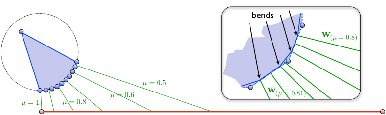
Figure 1: Two dimensional example of an SVM path with at least $\max(n_{+},n_{-})$ many bends. The green lines indicate the optimal solutions to the polytope distance problem (4), or equivalently the SVM formulations (2) and (3), for the indicated parameter value of $\mu$.

As $\mu$ decreases from $1$ down to $\frac{1}{2}$, the “left” end of the optimal distance vector, which is a multiple of the optimal $\mathbf{w}(\mu)$, walks through nearly all of the boundary faces of the blue class. More precisely, the number of bends in the path of the optimal $\mathbf{w}(\mu)$, for $1>\mu>\frac{1}{2}$, is at least twice the number of “inner” blue vertices, which is what we claimed above.

The above argument is not a formal proof, but it gives the main idea that will guide us in the high-dimensional construction. Going to higher dimensions will surprisingly not only allow us to prove a path complexity lower bound that is linear in the number of input points $n=n_{+}+n_{-}$, but even exponential in $n$ and also the dimension $d$ of the space containing the points.

4 The High-Dimensional Case

The idea is to spice up the two-dimensional example: we will construct two classes of $n_{+}=2d$ and $n_{-}=2$ points, respectively. The point sets will be in $\mathbb{R}^{d}$, but the construction ensures that for all relevant values of the parameter $\mu$, the two points of optimal distance are very close to the two-dimensional plane

$$\SS:=\{\mathbf{x}\in\mathbb{R}^{d}:x_{1}=\ldots=x_{d-2}=0\}.$$ (6)

The crucial feature of the construction is that the convex hull of the $n_{+}$ points intersects $\SS$ in a convex polygon with $2^{d}=2^{n_{+}/2}$ vertices and edges. Moreover, we “walk through” a constant fraction of them while changing the parameter $\mu$. We thus mimic the process depicted in Figure 1, except that the number of relevant bends is now exponential in $n_{+}$.

Our main technical tool is the well-known Goldfarb cube, a slightly deformed $d$-dimensional cube with $2d$ facets and $2^{d}$ vertices [2]. Its distinctive property is that all $2^{d}$ vertices are visible in the projection of the cube to $\SS$.

Taking the geometric dual of the Goldfarb cube (to be defined below), we obtain a $d$-dimensional polytope with $2d$ vertices and $2^{d}$ facets, all of which intersect our two-dimensional plane $\SS$. The $2d$ vertices of the dual Goldfarb cube then form our first point class, after applying a linear “stretching transform” that keeps our walk close to $\SS$.

4.1 Polytope Basics

Let us review some basic facts of polytope theory. For proofs, we refer to Ziegler’s standard textbook [53].

Every polytope can be defined in two ways: either as the convex hull of a finite set of points, or as the bounded solution set of finitely many linear inequalities. For a given polytope ${\cal P}$, an inequality $\mathbf{a}^{T}\mathbf{x}\leq b$ is called face-defining if $\mathbf{a}^{T}\mathbf{x}\leq b$ for all $\mathbf{x}\in{\cal P}$ and $\mathbf{a}^{T}\mathbf{x}=b$ for some $\mathbf{x}\in{\cal P}$. The set ${\cal F}=\{\mathbf{x}\in{\cal P}:\mathbf{a}^{T}\mathbf{x}=b\}$ is called the face of ${\cal P}$ defined by the inequality. If ${\cal P}$ has the origin in its interior, it suffices to consider inequalities of the form $\mathbf{a}^{T}\mathbf{x}\leq 1$. Faces of dimension $0$ are vertices, and faces of dimension $d-1$ are called facets. If ${\cal P}$ is full-dimensional, every vertex is the intersection of $d$ facets.

Every polytope is the convex hull of its vertices. More generally, every face ${\cal F}$ is the convex hull of the vertices contained in ${\cal F}$; in particular ${\cal F}$ is itself a polytope. This is implied by the following stronger property.

Lemma 1.

Let ${\cal P}=\mathop{{\rm conv}}({\cal V})\subseteq\mathbb{R}^{d}$ be a polytope with vertex set ${\cal V}$, and let ${\cal F}$ be a face of ${\cal P}$. For every point $\mathbf{p}\in{\cal P}$ and every convex combination

$$\mathbf{p}=\sum_{\mathbf{v}\in{\cal V}}\alpha_{\mathbf{v}}\mathbf{v},\quad\sum_{\mathbf{v}\in{\cal V}}\alpha_{\mathbf{v}}=1,\quad\alpha_{\mathbf{v}}\geq 0~{}\forall\mathbf{v}\in{\cal V},$$ (7)

the following two statements are equivalent.

• $\alpha_{\mathbf{v}}=0$ for all $\mathbf{v}\notin{\cal F}$.

• $\mathbf{p}\in{\cal F}$.

Proof.

Let $\mathbf{a}^{T}\mathbf{x}\leq b$ be some inequality that defines ${\cal F}$. If (i) holds, then (7) yields

$$\mathbf{a}^{T}\mathbf{p}=\sum_{\mathbf{v}\in{\cal V}\cap{\cal F}}\alpha_{\mathbf{v}}\underbrace{\mathbf{a}^{T}\mathbf{v}}_{=b}=b,$$

hence $\mathbf{p}\in{\cal F}$. For the other direction, let $\mathbf{p}\in{\cal F}$. We get

$$b=\mathbf{a}^{T}\mathbf{p}=\sum_{\mathbf{v}\in{\cal V}}\alpha_{\mathbf{v}}\underbrace{\mathbf{a}^{T}\mathbf{v}}_{\leq b}\leq\sum_{\mathbf{v}\in{\cal V}}\alpha_{\mathbf{v}}b=b,$$

where the inequality uses $\alpha_{\mathbf{v}}\geq 0~{}\forall\mathbf{v}\in{\cal V}$. It follows that the inequality is actually an equality, but this is possible only if $\alpha_{\mathbf{v}}=0$ whenever $\mathbf{a}^{T}\mathbf{v}<b\Leftrightarrow\mathbf{v}\notin{\cal F}$. ∎

4.2 The Goldfarb Cube

The $d$-dimensional Goldfarb cube is a slightly deformed variant of the cube $[-1,1]^{d}\subseteq\mathbb{R}^{d}$. More precisely, it is a polytope given as the solution set of the following $2d$ linear inequalities.

Definition 1.

For fixed $\epsilon$ and $\gamma$ such that $0<4\gamma<\epsilon<\frac{1}{2}$, the Goldfarb cube $\mathrm{Gol}_{d}$ is the set of points $\mathbf{x}=(x_{1},\ldots,x_{d})^{T}\in\mathbb{R}^{d}$ satisfying the $2d$ linear inequalities

$$\begin{array}[]{rcccl}-z_{1}&\leq&x_{1}&\leq&z_{1}:=1,\\ -z_{2}&\leq&x_{2}&\leq&z_{2}:=1-\epsilon-\epsilon x_{1},\\ -z_{k}&\leq&x_{k}&\leq&z_{k}:=1-\epsilon+\epsilon\gamma-\epsilon(x_{k-1}-\gamma x_{k-2}),\quad 3\leq k\leq d.\end{array}$$ (8)

We note that the “standard” Goldfarb cube as in [2] is defined differently but can be obtained from our variant by translation and scaling: under the coordinate transformation $x_{k}=2x^{\prime}_{k}-1$, (8) is equivalent to Amenta & Ziegler’s Goldfarb cube inequalities [2]. The Goldfarb cube was originally constructed to get a linear program on which the simplex algorithm with the shadow vertex pivot rule needs an exponential number of steps to find the optimal solution [20].

In the following, we state some important properties of the Goldfarb cube; proofs can be found in [2].

$\mathrm{Gol}_{d}$ is a full-dimensional polytope with $2d$ facets and the origin in its interior (this actually holds for all $\epsilon<1$). For each $k=1,\ldots,d$, the two inequalities $-z_{k}\leq x_{k}\leq z_{k}$ of (8) define two disjoint “opposite” facets. A vertex is therefore the intersection of exactly $d$ facets, one from each pair of opposite facets. In fact, every such choice of $d$ facets yields a distinct vertex which means that there are $2^{d}$ vertices that can be indexed by the set $\{-1,1\}^{d}$. An index vector $\sigma\in\{-1,1\}^{d}$ tells us for each pair $-z_{k}\leq x_{k}\leq z_{k}$ of inequalities whether the left one is tight at the vertex ($\sigma_{k}=-1$), or the right one ($\sigma_{k}=1$). We can therefore easily compute the vertices.

Lemma 2.

Let $\sigma\in\{-1,1\}^{d}$. The vector $\mathbf{x}=(x_{1},\ldots,x_{d})^{T}$ given by

$$\begin{array}[]{rcl}x_{1}&=&\sigma_{1},\\ x_{2}&=&\sigma_{2}(1-\epsilon-\epsilon x_{1}),\\ x_{k}&=&\sigma_{k}(1-\epsilon+\epsilon\gamma-\epsilon(x_{k-1}-\gamma x_{k-2})),\quad k=3,\ldots,d,\end{array}$$ (9)

is a vertex of $\mathrm{Gol}_{d}$ and will be denoted by $\mathbf{v}_{\sigma}$.

Corollary 3.

Fix $\sigma\in\{-1,1\}^{d}$ and consider the vertex $\mathbf{v}_{\sigma}=(v_{\sigma,1},\ldots,v_{\sigma,d})^{T}$. Then

$$\mathop{{\rm sign}}(v_{\sigma,k})=\sigma_{k},\quad 1\leq k\leq d.$$

Proof.

Since all the $\mathbf{v}_{\sigma}$’s are distinct, (9) shows that we must in particular have $v_{\sigma,k}\neq v_{\sigma^{\prime},k}$ if $\sigma^{\prime}$ differs from $\sigma$ in the $k$-th coordinate only. Writing the expression for $x_{k}$ in (9) as $x_{k}=\pm z_{k}$, we thus get

$$-z_{k}=\min(v_{\sigma,k},v_{\sigma^{\prime},k})<\max(v_{\sigma,k},v_{\sigma^{\prime},k})=z_{k},$$

showing that $z_{k}>0$. It follows that $\mathop{{\rm sign}}(v_{\sigma,k})=\mathop{{\rm sign}}(\sigma_{k}z_{k})=\mathop{{\rm sign}}(\sigma_{k})$. ∎

Now we are ready to state the crucial property of the Goldfarb cube (which is invariant under translation and scaling, hence it applies to our as well as the “standard” variant of the Goldfarb cube).

Theorem 4 (Theorem 4.4 in [2]).

Let $\pi:\mathbb{R}^{d}\rightarrow\mathbb{R}^{2}$ be the projection onto the last two coordinates, i.e.

$$\pi((x_{1},x_{2},\ldots,x_{d-2},x_{d-1},x_{d})^{T})=(x_{d-1},x_{d})^{T}.$$

The projection $\pi(\mathrm{Gol}_{d})=\{\pi(\mathbf{x}):\mathbf{x}\in\mathrm{Gol}_{d}\}$ is a convex polygon (two-dimensional polytope) with $2^{d}$ distinct vertices $\{\pi(\mathbf{v}_{\sigma}):\sigma\in\{-1,1\}^{d}\}$. In formulas, for every $\sigma\in\{-1,1\}^{d}$, there exists an inequality $\mathbf{a}^{T}\mathbf{x}\leq 1$ such that $\mathbf{a}\in\SS$ (recall that $\SS$ is the two-dimensional plane defined in (6)) and

$$\begin{array}[]{lclclcl}\mathbf{a}^{T}\mathbf{v}_{\sigma}&=&a_{d-1}v_{\sigma,d-1}&+&a_{d}v_{\sigma,d}&=&1,\\ \mathbf{a}^{T}\mathbf{x}&=&a_{d-1}x_{d-1}&+&a_{d}x_{d}&<&1,\quad\mathbf{x}\in\mathrm{Gol}_{d}\setminus\{\mathbf{v}_{\sigma}\}.\end{array}$$

This precisely means that the inequality

$$a_{d-1}x+a_{d}y\leq 1$$

defines the vertex $\pi(\mathbf{v}_{\sigma})=(v_{\sigma,d-1},v_{\sigma,d})^{T}$ of $\pi(\mathrm{Gol}_{d})=\{(x_{d-1},x_{d})^{T}:\mathbf{x}\in\mathrm{Gol}_{d}\}$.

The set $\pi(\mathrm{Gol}_{d})$ is the shadow of $\mathrm{Gol}_{d}$ under the projection $\pi$, and the theorem tells us that all Goldfarb cube vertices appear on the boundary of the shadow. “Usually”, the shadow of a polytope is of much smaller complexity, since many vertices project to its interior.

4.3 Geometric Duality

There is a natural bijective transformation ${\cal D}$ that maps points $\mathbf{p}=(p_{1},\ldots,p_{d})$ to inequalities strictly satisfied by $\mathbf{0}$:

$${\cal D}:(p_{1},p_{2},\ldots,p_{d})^{T}\mapsto\{\mathbf{x}\in\mathbb{R}^{d}:\mathbf{p}^{T}\mathbf{x}\leq 1\}.$$

Using ${\cal D}$, we can map every set ${\cal P}\subseteq\mathbb{R}^{d}$ to its dual (sometimes also called the polar set)

$${\cal P}^{\triangle}:=\bigcap_{\mathbf{p}\in{\cal P}}\{\mathbf{x}\in\mathbb{R}^{d}:\mathbf{p}^{T}\mathbf{x}\leq 1\}.$$

If ${\cal P}$ is a polytope with $\mathbf{0}\in\mathop{\rm int}({\cal P})$, given as the convex hull of a finite set of points ${\cal V}$, then it can be shown that

$${\cal P}^{\triangle}=\bigcap_{\mathbf{v}\in{\cal V}}\{\mathbf{x}\in\mathbb{R}^{d}:\mathbf{v}^{T}\mathbf{x}\leq 1\}.$$ (10)

This means, ${\cal P}^{\triangle}$ is also a polytope, given as the solution set of finitely many linear inequalities (boundedness follows from $\mathbf{0}\in\mathop{\rm int}({\cal P})$).

This duality transform has two interesting properties that we need.

Proposition 1.

Let ${\cal P}\subseteq\mathbb{R}^{d}$ be a polytope containing the origin in its interior, and let ${\cal P}^{\triangle}$ be its dual polytope.

• ${\cal P}=({\cal P}^{\triangle})^{\triangle}$, i.e. the dual of the dual is the original polytope.

• If ${\cal P}$ has $N$ vertices and $M$ facets, then ${\cal P}^{\triangle}$ has $M$ vertices and $N$ facets. More precisely, $\mathbf{v}$ is a vertex of one of the polytopes if and only if the inequality $\mathbf{v}^{T}\mathbf{x}\leq 1$ defines a facet of the other.

As simple examples, we may consider the three-dimensional platonic solids. The geometric dual of a tetrahedron is again a tetrahedron. A cube is dual to an octahedron, and a dodecahedron is dual to an icosahedron. The geometric dual of the $d$-dimensional unit cube is the cross-polytope, having $2d$ vertices and $2^{d}$ facets. The dual of the Goldfarb cube is therefore a perturbed version of the cross-polytope, see Figure 2.

4.4 The Dual Goldfarb Cube

We are now able to follow up on our initial idea outlined in the beginning of Section 4. By Proposition 1(ii), the dual Goldfarb cube $\mathrm{Gol}^{\triangle}_{d}$ has $2d$ vertices and $2^{d}$ facets. Moreover, we now easily see that all $2^{d}$ facets intersect the two-dimensional plane $\SS$ defined in (6). We in fact already know points of $\SS$ in each of these facets.

Corollary 5 (of Theorem 4).

Let $\sigma\in\{-1,1\}^{d}$. For the point $\mathbf{a}=:\mathbf{p}_{\sigma}\in\SS$ as constructed in Theorem 4, we have

$$\mathbf{p}_{\sigma} \in \mathrm{Gol}^{\triangle}_{d}\cap\SS,$$ (11)

$$\mathbf{p}_{\sigma}^{T}\mathbf{v}_{\sigma} = 1,$$ (12)

$$\mathbf{p}_{\sigma}^{T}\mathbf{v}_{\tau} < 1,\quad\tau\neq\sigma.$$ (13)

This means that $\mathbf{p}_{\sigma}$ is in the $\sigma$-facet of $\mathrm{Gol}^{\triangle}_{d}$ defined by the inequality $\mathbf{v}_{\sigma}^{T}\mathbf{x}\leq 1$, but not in any other facet.

Proof.

Theorem 4 readily guarantees $\mathbf{p}_{\sigma}\in\SS$. Now we use the other two properties of $\mathbf{p}_{\sigma}$ from the theorem:

$$\mathbf{p}_{\sigma}^{T}\mathbf{v}_{\sigma} = 1,$$

$$\mathbf{p}_{\sigma}^{T}\mathbf{x} < 1,\quad\mathbf{x}\in\mathrm{Gol}_{d}\setminus\{\mathbf{v}_{\sigma}\}.$$

The first one is (12), and using the second one with $\mathbf{x}=\mathbf{v}_{\tau}$ yields (13). Both properties together show that

$$\mathbf{p}_{\sigma}\in\mathrm{Gol}^{\triangle}_{d}=\bigcap_{\tau\in\{-1,1\}^{d}}\{\mathbf{x}\in\mathbb{R}^{d}:\mathbf{v}_{\tau}^{T}\mathbf{x}\leq 1\},$$

where we are using (10) and Proposition 1(ii). ∎

We will need the following fact about the polygon $\mathrm{Gol}^{\triangle}_{d}\cap\SS$.

Lemma 6.

Let $\mathbf{x}\in\mathrm{Gol}^{\triangle}_{d}\cap\SS$. Then $x_{d-1}\leq 1$.

Proof.

By applying the definition of the dual polytope for the choice of two particular vertices $\mathbf{v}_{\sigma}\in\mathrm{Gol}_{d}$ of the Goldfarb cube as defined in (9), we have that for all $\mathbf{x}\in\mathrm{Gol}^{\triangle}_{d}$,

$$\mathbf{v}_{(-1,\ldots,-1,1,-1)}^{T}\mathbf{x} = (-1,\ldots,-1,1,-1+2\epsilon)^{T}\mathbf{x}\leq 1,$$

$$\mathbf{v}_{(-1,\ldots,-1,1,+1)}^{T}\mathbf{x} = (-1,\ldots,-1,1,+1-2\epsilon)^{T}\mathbf{x}\leq 1.$$

Summing up both inequalities yields $(-2,\ldots,-2,2,0)^{T}\mathbf{x}\leq 2$, meaning that $x_{d-1}\leq 1$ if $\mathbf{x}\in\SS$. ∎

We will also need the vertices of the dual Goldfarb cube. By geometric duality, they are in one-to-one correspondence with the facets of $\mathrm{Gol}_{d}$. Both can be indexed by the set $\{1,\ldots,d\}\times\{-1,1\}$ as follows:

Definition 2.

For $(k,s)\in\{1,\ldots,d\}\times\{-1,1\}$, let $\mathbf{w}_{(k,s)}\in\mathbb{R}^{d}$ be the unique vector such that for $s=-1$, the inequality $-z_{k}\leq x_{k}$ in (8) and for $s=1$ the inequality $x_{k}\leq z_{k}$ assumes the form

$$\mathbf{w}_{(k,s)}^{T}\mathbf{x}\leq 1.$$

According to Proposition 1 (ii), the set

$$\{\mathbf{w}_{(k,s)}:1\leq k\leq d,~{}s\in\{-1,1\}\}$$

is exactly the set of the $2d$ vertices of the dual Goldfarb cube $\mathrm{Gol}^{\triangle}_{d}$.

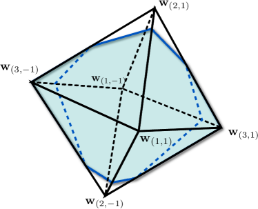
Figure 2: The dual of the Goldfarb cube in $3$ dimensions is the perturbed cross-polytope $\mathrm{Gol}^{\triangle}_{3}$. If we imagine the vertices $\mathbf{w}_{(2,1)}$ and $\mathbf{w}_{(2,-1)}$ lying just slightly behind the intersection plane $\SS$, and the vertices $\mathbf{w}_{(3,1)}$ and $\mathbf{w}_{(3,-1)}$ just slightly in front of $\SS$, then the plane $\SS$ intersects all $2^{3}=8$ triangular facets.

4.5 Stretching

Ideally, we would now like to use the vertices of the dual Goldfarb cube $\mathrm{Gol}^{\triangle}_{d}$ as our first class of $n_{+}=2d$ points, and make sure that the solution path “walks along” the exponentially many facets that intersect the two-dimensional plane $\SS$ according to Corollary 5. But for that, we need the walk to stay close to $\SS$. To achieve this, we still need to “stretch” $\mathrm{Gol}^{\triangle}_{d}$ such that its facets are almost orthogonal to $\SS$. The stretching transform scales all coordinates except the last two by some fixed number $L$ (considered large).

Definition 3.

For $\mathbf{x}=(x_{1},\ldots,x_{d})^{T}\in\mathbb{R}^{d}$ and $L\geq 0$ a real number, we define

$$\mathbf{x}(L)=(Lx_{1},\ldots,Lx_{d-2},x_{d-1},x_{d}).$$

For a set ${\cal P}\subseteq\mathbb{R}^{d}$,

$${\cal P}(L):=\{\mathbf{x}(L):\mathbf{x}\in{\cal P}\}$$

is the $L$-stretched version of ${\cal P}$.

The following is a straightforward consequence of this definition; we omit the proof.

Observation 1.

Let ${\cal P}$ be a polytope and ${\cal P}(L)$ its $L$-stretched version, $L\geq 0$.

• ${\cal P}\cap\SS={\cal P}(L)\cap\SS$, where $\SS$ is the two-dimensional plane defined in (6).

• For $L>0$, the inequality $\mathbf{a}^{T}\mathbf{x}\leq 1$ defines the face ${\cal F}$ of ${\cal P}$ if and only if the inequality $\mathbf{a}(1/L)^{T}\mathbf{x}\leq 1$ defines the face ${\cal F}(L)$ of ${\cal P}(L)$.

• For $L>0$, the point $\mathbf{v}$ is a vertex of ${\cal P}$ if and only if the point $\mathbf{v}(L)$ is a vertex of ${\cal P}(L)$.

The idea behind the stretching transform is that for $L$ large enough, the projection of any given point $\mathbf{q}\in\SS$ onto $\mathrm{Gol}^{\triangle}_{d}(L)$ is close to $\SS$. The following is the key lemma; $\ell$ assumes the role of $1/L$.

Lemma 7.

Let $\mathbf{a}\in\mathbb{R}^{d}$ such that $(a_{d-1},a_{d})\neq\mathbf{0}$. Fix a point $\mathbf{q}\in\SS$ such that $\mathbf{a}^{T}\mathbf{q}>1$. For a real number $\ell\geq 0$, let $\mathbf{p}^{(\ell)}$ be the projection (formally defined in the proof below) of $\mathbf{q}$ onto the equality $\mathbf{a}(\ell)^{T}\mathbf{x}=1$. Then

$$\lim_{\ell\rightarrow 0}\mathbf{p}^{(\ell)}=\mathbf{p}^{(0)}\in\SS.$$

Proof.

The projection $\mathbf{p}^{(\ell)}$ can be defined through the equations

$$\mathbf{a}(\ell)^{T}\mathbf{p}^{(\ell)}=1,\quad\mathbf{p}^{(\ell)}-\mathbf{q}=t~{}\mathbf{a}(\ell)\mbox{~{}~{}for some $t$}.$$ (14)

This is equivalent to

$$\mathbf{p}^{(\ell)}=C\frac{\mathbf{a}(\ell)}{\|\mathbf{a}(\ell)\|^{2}}+\mathbf{q},\mbox{~{}~{}with~{}~{}}C:=1-\mathbf{a}(\ell)^{T}\mathbf{q}=1-\mathbf{a}^{T}\mathbf{q}<0.$$ (15)

Now, since $\mathbf{a}(\ell)$ converges to $\mathbf{a}(0)$ and $\|\mathbf{a}(\ell)\|^{2}$ converges to $\|\mathbf{a}(0)\|^{2}\neq 0$, the claim follows; $\mathbf{p}^{(0)}\in\SS$ is a consequence of $\mathbf{q},\mathbf{a}(0)\in\SS$ and (15). ∎

4.6 Many Optimal Pairs

Let us now fix a sufficiently large stretch factor $L$ and its inverse $\ell=1/L$. The goal of this section is to construct a line ${\cal L}\subseteq\SS$, disjoint from $\mathrm{Gol}^{\triangle}_{d}(L)$, such that for exponentially many $\sigma\in\{-1,1\}^{d}$, we find a pair of points $({\mathbf{p}_{\sigma}^{(\ell)}},{\mathbf{q}_{\sigma}})$, ${\mathbf{p}_{\sigma}^{(\ell)}}\in\mathrm{Gol}^{\triangle}_{d}(L),{\mathbf{q}_{\sigma}}\in{\cal L}$, with the following properties.

• ${\mathbf{p}_{\sigma}^{(\ell)}}$ is in the $\sigma$-facet of the stretched dual Goldfarb cube, and in no other facet; and

• $({\mathbf{p}_{\sigma}^{(\ell)}},{\mathbf{q}_{\sigma}})$ is the unique pair of closest distance between the stretched dual Goldfarb cube and the ray $\{\mathbf{x}\in{\cal L}:x_{d}\geq q_{\sigma,d}\}$.

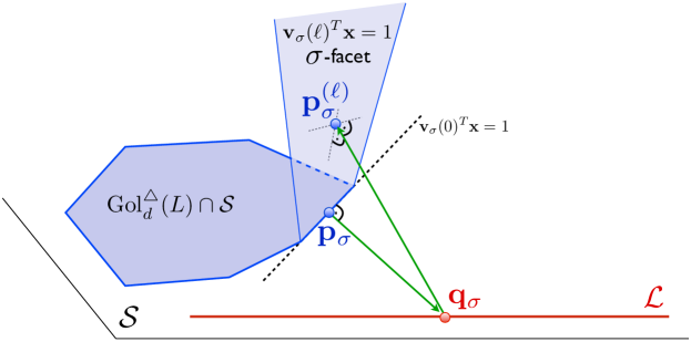
Figure 3: Obtaining the two points ${\mathbf{p}_{\sigma}^{(\ell)}}$ and ${\mathbf{q}_{\sigma}}$ by first “projecting” $\mathbf{p}_{\sigma}$ onto the line ${\cal L}$ and then back onto the $\sigma$-facet of the polytope $\mathrm{Gol}^{\triangle}_{d}(L)$.

4.6.1 The Line

The first step is to define the line ${\cal L}$. We choose

$${\cal L}:=\{(0,\ldots,0,2,y)^{T}:y\in\mathbb{R}\}\subseteq\SS.$$ (16)

This line is disjoint from $\mathrm{Gol}^{\triangle}_{d}(L)$ by Lemma 6.

4.6.2 The Point ${\mathbf{q}_{\sigma}}$

Let us now fix $\sigma\in\{-1,1\}^{d}$ such that $\sigma_{d-1}=1$. According to Corollary 3, the Goldfarb cube vertex $\mathbf{v}_{\sigma}$ satisfies $v_{\sigma,d-1}>0$.

We start with the point $\mathbf{p}_{\sigma}\in\mathrm{Gol}^{\triangle}_{d}\cap\SS$ constructed in Corollary 5. This point is in the $\sigma$-facet of $\mathrm{Gol}^{\triangle}_{d}$ defined by the inequality $\mathbf{v}_{\sigma}^{T}\mathbf{x}\leq 1$. We next find a point ${\mathbf{q}_{\sigma}}\in{\cal L}$ such that $\mathbf{p}_{\sigma}$ is the projection of ${\mathbf{q}_{\sigma}}$ onto the “vertical” inequality $\mathbf{v}_{\sigma}(0)^{T}\mathbf{x}\leq 1$. See also Figure 3 for an illustration. According to (15), ${\mathbf{q}_{\sigma}}$ must satisfy

$$\mathbf{p}_{\sigma}=C\frac{\mathbf{v}_{\sigma}(0)}{\|\mathbf{v}_{\sigma}(0)\|^{2}}+{\mathbf{q}_{\sigma}},\quad C=1-\mathbf{v}_{\sigma}(0)^{T}{\mathbf{q}_{\sigma}}<0.$$ (17)

To get ${\mathbf{q}_{\sigma}}$, we thus simply define

$${\mathbf{q}_{\sigma}}:=\mathbf{p}_{\sigma}-C\frac{\mathbf{v}_{\sigma}(0)}{\|\mathbf{v}_{\sigma}(0)\|^{2}}\in\SS,$$ (18)

where $C$ is chosen such that $q_{\sigma,d-1}=2$. This is possible since $v_{\sigma,d-1}\neq 0$. Premultiplying with $\mathbf{v}_{\sigma}(0)^{T}$ shows that

$$C=\underbrace{\mathbf{v}_{\sigma}(0)^{T}\mathbf{p}_{\sigma}}_{=\mathbf{v}_{\sigma}^{T}\mathbf{p}_{\sigma}=1}-\mathbf{v}_{\sigma}(0)^{T}{\mathbf{q}_{\sigma}}=1-\mathbf{v}_{\sigma}(0)^{T}{\mathbf{q}_{\sigma}},$$

as required. Also, by using Lemma 6 and the defining equation (18), we obtain that $C<0$, as a consequence of

$$q_{\sigma,d-1}=2=\underbrace{p_{\sigma,d-1}}_{\leq 1}-C\underbrace{v_{\sigma,d-1}}_{>0}.$$

4.6.3 The Point ${\mathbf{p}_{\sigma}^{(\ell)}}$

With ${\mathbf{q}_{\sigma}}$ as previously defined, we now define ${\mathbf{p}_{\sigma}^{(\ell)}}$ by projecting ${\mathbf{q}_{\sigma}}$ back onto the $\sigma$-facet of our polytope, the stretched dual Goldfarb cube, see also Figure 3. Formally we set

$${\mathbf{p}_{\sigma}^{(\ell)}}:=C\frac{\mathbf{v}_{\sigma}(\ell)}{\|\mathbf{v}_{\sigma}(\ell)\|^{2}}+{\mathbf{q}_{\sigma}},\quad C:=1-\mathbf{v}_{\sigma}(\ell)^{T}{\mathbf{q}_{\sigma}}=1-\mathbf{v}_{\sigma}(0)^{T}{\mathbf{q}_{\sigma}}<0.$$ (19)

By (15), ${\mathbf{p}_{\sigma}^{(\ell)}}$ is now the projection of ${\mathbf{q}_{\sigma}}$ onto the inequality $\mathbf{v}_{\sigma}(\ell)^{T}\mathbf{x}\leq 1$ defining the $\sigma$-facet of $\mathrm{Gol}^{\triangle}_{d}(L)$.

4.6.4 Optimality of $({\mathbf{p}_{\sigma}^{(\ell)}},{\mathbf{q}_{\sigma}})$

For the pair $({\mathbf{p}_{\sigma}^{(\ell)}},{\mathbf{q}_{\sigma}})$, items (i) and (ii) of the plan outlined in the beginning of Section 4.6 remain to be proved. We do this by the following main theorem, showing that the construction works for $1/4$ of all choices of $\sigma$’s.

Theorem 8.

For $\sigma\in\{-1,1\}^{d}$ such that $\sigma_{d-1}=\sigma_{d}=1$, let ${\mathbf{q}_{\sigma}}$ and ${\mathbf{p}_{\sigma}^{(\ell)}}$ be as defined in (18) and (19). For sufficiently small $\ell:=1/L>0$, the following two statements hold.

• ${\mathbf{p}_{\sigma}^{(\ell)}}\in\mathrm{Gol}^{\triangle}_{d}(L)$; in particular,

  $$\mathbf{v}_{\sigma}(\ell)^{T}{\mathbf{p}_{\sigma}^{(\ell)}} = 1,$$

  $$\mathbf{v}_{\tau}(\ell)^{T}{\mathbf{p}_{\sigma}^{(\ell)}} < 1,\quad\tau\neq\sigma.$$

• The pair $(\mathbf{x},\mathbf{x}^{\prime})=({\mathbf{p}_{\sigma}^{(\ell)}},{\mathbf{q}_{\sigma}})$ is the unique optimal solution of the optimization problem

  $$\begin{array}[]{ll}\mathop{{\rm minimize}}_{\mathbf{x},\mathbf{x}^{\prime}}&\|\mathbf{x}-\mathbf{x}^{\prime}\|\\ \mathop{{\rm subject~{}to}}&\mathbf{x}\in\mathrm{Gol}^{\triangle}_{d}(L)\\ &\mathbf{x}^{\prime}\in{\cal L}\\ &x^{\prime}_{d}\geq q_{\sigma,d}.\end{array}$$ (20)

Proof.

We have

$${\mathbf{p}_{\sigma}^{(\ell)}}^{T}\mathbf{v}_{\sigma}(\ell)=1$$

by definition of ${\mathbf{p}_{\sigma}^{(\ell)}}$, see (14). As a consequence of (13), the point $\mathbf{p}_{\sigma}\in\SS$ satisfies

$$\mathbf{p}_{\sigma}^{T}\mathbf{v}_{\tau}(0)=\mathbf{p}_{\sigma}^{T}\mathbf{v}_{\tau}<1,\quad\tau\neq\sigma.$$ (21)

Due to $\displaystyle\lim_{\ell\rightarrow 0}\mathbf{p}_{\sigma}^{(\ell)}=\mathbf{p}_{\sigma}$ (here we use $\mathbf{p}_{\sigma}^{(0)}=\mathbf{p}_{\sigma}$, see the “Ansatz” (17), and Lemma 7), we also have

$$\lim_{\ell\rightarrow 0}{\mathbf{p}_{\sigma}^{(\ell)}}^{T}\mathbf{v}_{\tau}(\ell)=\mathbf{p}_{\sigma}^{T}\mathbf{v}_{\tau}(0)<1,$$ (22)

hence ${\mathbf{p}_{\sigma}^{(\ell)}}^{T}\mathbf{v}_{\tau}(\ell)<1$ for sufficiently small $\ell$, and this proves part (i) of the theorem.

For the second part, we first observe that the problem (20) can be written as a quadratic program, the problem of minimizing a convex quadratic function subject to linear (in)equality constraints. Indeed, after squaring the objective function, we obtain the following equivalent program:

$$\begin{array}[]{lrcl}\mathop{{\rm minimize}}_{\mathbf{x},\mathbf{x}^{\prime}}&(\mathbf{x}-\mathbf{x}^{\prime})^{T}(\mathbf{x}-\mathbf{x}^{\prime})\\ \mathop{{\rm subject~{}to}}&\mathbf{v}_{\tau}(\ell)^{T}\mathbf{x}&\leq&1,\quad\tau\in\{-1,1\}^{d}\\ &x^{\prime}_{i}&=&0,\quad i=1,\ldots,d-2\\ &x^{\prime}_{d-1}&=&2\\ &x^{\prime}_{d}&\geq&q_{\sigma,d}.\end{array}$$ (23)

For quadratic programs, the Karush-Kuhn-Tucker optimality conditions [39] are necessary and sufficient for the existence of an optimal solution. Here, these conditions assume the following form: a feasible solution $(\mathbf{x},\mathbf{x}^{\prime})$ of (23) is optimal if and only if there exist real numbers $\lambda_{\tau}\geq 0,\tau\in\{-1,1\}^{d}$ and a vector $\mathbf{\Lambda}\in\mathbb{R}^{d}$, $\Lambda_{d}\leq 0$ such that

$$2(\mathbf{x}-\mathbf{x}^{\prime})+\sum_{\tau\in\{-1,1\}^{d}}\lambda_{\tau}\mathbf{v}_{\tau}(\ell) = 0$$ (24)

$$2(\mathbf{x}^{\prime}-\mathbf{x})+\mathbf{\Lambda} = 0$$ (25)

$$\lambda_{\tau}(\mathbf{v}_{\tau}(\ell)^{T}\mathbf{x}-1) = 0,\quad\tau\in\{-1,1\}^{d},$$ (26)

$$\Lambda_{d}(x^{\prime}_{d}-q_{\sigma,d}) = 0.$$ (27)

This easily yields that $(\mathbf{x},\mathbf{x}^{\prime})=({\mathbf{p}_{\sigma}^{(\ell)}},{\mathbf{q}_{\sigma}})$ is indeed an optimal pair. According to (19), ${\mathbf{p}_{\sigma}^{(\ell)}}-{\mathbf{q}_{\sigma}}$ is a negative multiple of $\mathbf{v}_{\sigma}(\ell)$, hence we may choose $\lambda_{\sigma}>0$ and $\lambda_{\tau}=0,\tau\neq\sigma$ such that (24) is satisfied. To satisfy (25), we simply set $\mathbf{\Lambda}=2({\mathbf{p}_{\sigma}^{(\ell)}}-{\mathbf{q}_{\sigma}})$ and observe that indeed $\Lambda_{d}\leq 0$ since $\Lambda_{d}=p_{d}-q_{\sigma,d}$ is a negative multiple of $v_{\sigma,d}(\ell)=v_{\sigma,d}>0$ by our choice of $\sigma_{d}=1$ and Corollary 3. The last two complementary slackness conditions (26) and (27) are satisfied due to $\mathbf{v}_{\sigma}(\ell)^{T}{\mathbf{p}_{\sigma}^{(\ell)}}=1$ and $\mathbf{x}^{\prime}={\mathbf{q}_{\sigma}}$.

It remains to show that $({\mathbf{p}_{\sigma}^{(\ell)}},{\mathbf{q}_{\sigma}})$ is the unique optimal pair. We actually prove a stronger property: $({\mathbf{p}_{\sigma}^{(\ell)}},{\mathbf{q}_{\sigma}})$ is the unique optimal solution of the following relaxed problem, obtained after dropping all inequalities $\mathbf{v}_{\tau}(\ell)^{T}\mathbf{x}\leq 1$ for $\tau\neq\sigma$.

$$\begin{array}[]{lrcl}\mathop{{\rm minimize}}_{\mathbf{x},\mathbf{x}^{\prime}}&(\mathbf{x}-\mathbf{x}^{\prime})^{T}(\mathbf{x}-\mathbf{x}^{\prime})\\ \mathop{{\rm subject~{}to}}&\mathbf{v}_{\sigma}(\ell)^{T}\mathbf{x}&\leq&1\\ &x^{\prime}_{i}&=&0,\quad i=1,\ldots,d-2\\ &x^{\prime}_{d-1}&=&2\\ &x^{\prime}_{d}&\geq&q_{\sigma,d}.\end{array}$$ (28)

First we prove that the relaxed problem has no other optimal solution of the form $(\mathbf{p},{\mathbf{q}_{\sigma}})$. Due to $\mathbf{v}_{\sigma}(\ell)^{T}{\mathbf{q}_{\sigma}}>1$, see (19), we cannot have $\mathbf{p}={\mathbf{q}_{\sigma}}$. Then, the Karush-Kuhn-Tucker conditions

$$2(\mathbf{x}-\mathbf{x}^{\prime})+\lambda_{\sigma}\mathbf{v}_{\sigma}(\ell)^{T} = 0,\quad\lambda_{\sigma}\geq 0$$

$$2(\mathbf{x}^{\prime}-\mathbf{x})+\mathbf{\Lambda} = 0,\quad\Lambda_{d}\leq 0$$

$$\lambda_{\sigma}(\mathbf{v}_{\sigma}(\ell)^{T}\mathbf{x}-1) = 0$$

$$\Lambda_{d}(x^{\prime}_{d}-q_{\sigma,d}) = 0$$

for the relaxed problem require $\mathbf{p}-{\mathbf{q}_{\sigma}}$ to be a strictly negative multiple of $\mathbf{v}_{\sigma}(\ell)$. Complementary slackness in turn implies $\mathbf{v}_{\sigma}(\ell)^{T}\mathbf{p}=1$, and according to (19), this already determines $\mathbf{p}={\mathbf{p}_{\sigma}^{(\ell)}}$, see the definition of projection (14). To rule out an optimal solution $(\mathbf{p},\mathbf{q})$ with $\mathbf{q}\neq{\mathbf{q}_{\sigma}}$, we observe that $q_{d}>q_{\sigma,d}$ implies $\Lambda_{d}=0$ in the Karush-Kuhn-Tucker conditions by complementary slackness. This in turn yields $p_{d}=q_{d}$ and hence $\lambda_{\sigma}=0$ because $v_{\sigma,d}(\ell)>0$. But then $\mathbf{p}=\mathbf{q}$ which cannot be a solution because of

$$\mathbf{v}_{\sigma}(\ell)^{T}\mathbf{q}=v_{\sigma,d-1}2+\underbrace{v_{\sigma,d}}_{>0}q_{d}\geq v_{\sigma,d-1}2+v_{\sigma,d}q_{\sigma,d}=\mathbf{v}_{\sigma}(\ell)^{T}{\mathbf{q}_{\sigma}}>1.\vspace{-1em}$$

∎

We still need to show that we have actually obtained “many different optimal pairs”. But his is easy now.

Corollary 9.

All points ${\mathbf{p}_{\sigma}^{(\ell)}}$ considered in Theorem 8 are pairwise distinct, and so are all the points ${\mathbf{q}_{\sigma}}$.

Proof.

Pairwise distinctness of the ${\mathbf{p}_{\sigma}^{(\ell)}}$ immediately follows from statetment (i) of Theorem 8. If we assume that $\mathbf{q}_{\sigma}=\mathbf{q}_{\sigma^{\prime}}$ for $\sigma\neq\sigma^{\prime}$, then $({\mathbf{p}_{\sigma}^{(\ell)}},{\mathbf{q}_{\sigma}})$ and $(\mathbf{p}_{\sigma^{\prime}}^{(\ell)},\mathbf{q}_{\sigma^{\prime}})$ are distinct optimal pairs for (20) which contradicts statement (ii) of Theorem 8. ∎

4.6.5 Constructing Support Vectors

As we have outlined in the introductory Section 2.1, it is standard that any solution to an SVM-like optimization problem can be expressed in two ways: either as an explicit vector solving the primal SVM problem (2) or the distance version (4), or secondly as a convex combination of the input points, if we consider the corresponding dual problem, which in our case is (3). The input points appearing with non-zero coefficient in such a convex combination are called the support vectors.

For polytope distance problems, these two representations are even easier to see and convert into each other, as a point is in a polytope if and only if it is a convex combination of the vertices of the polytope, see also the polytope basics in Section 4.1.

We will now show that when using the stretched dual Goldfarb cube $\mathrm{Gol}^{\triangle}_{d}(L)$ as one point class of a polytope distance problem, then the support vectors of the point ${\mathbf{p}_{\sigma}^{(\ell)}}$ as constructed in Section 4.6.3 are precisely the $d$ vertices $\mathbf{w}_{(k,\sigma_{k})}(L)$ of $\mathrm{Gol}^{\triangle}_{d}(L)$. This means that for every chosen $\sigma\in\{-1,1\}^{d}$, we will get a different set of support vectors for ${\mathbf{p}_{\sigma}^{(\ell)}}$. The following general lemma lets us express a point $\mathbf{p}\in\mathrm{Gol}^{\triangle}_{d}(L)$ as a unique convex combination of its support vectors. Due to Theorem 8, this lemma will in particular apply to our solution points ${\mathbf{p}_{\sigma}^{(\ell)}}$.

Lemma 10.

Let $\sigma\in\{-1,1\}^{d}$, and $\mathbf{p}\in\mathrm{Gol}^{\triangle}_{d}(L)$ such that

$$\mathbf{v}_{\sigma}(\ell)^{T}\mathbf{p} = 1,$$

$$\mathbf{v}_{\tau}(\ell)^{T}\mathbf{p} < 1,\quad\tau\neq\sigma,$$

where $\ell=1/L$. Then we can write $\mathbf{p}$ as a convex combination of exactly $d$ vertices, namely

$$\mathbf{p}=\sum_{k=1}^{d}\alpha_{(k,\sigma_{k})}\mathbf{w}_{(k,\sigma_{k})}(L),\quad\sum_{k=1}^{d}\alpha_{(k,\sigma_{k})}=1,\quad\alpha_{(k,\sigma_{k})}>0~{}\forall k.$$ (29)

Moreover, this convex combination is unique among all convex combinations of the $2d$ vertices $\mathbf{w}_{(k,s)}(L)$, for $k\in\{1,\dots,d\}$ and $s\in\{-1,1\}$.

Proof.

$\mathrm{Gol}^{\triangle}_{d}(L)$ is the convex hull of its $2d$ many vertices $\mathbf{w}_{(k,s)}(L)$, see Section 4.1, Definition 2 and Observation 1. This means that $\mathbf{p}$ can be written as some convex combination of the form

$$\mathbf{p}=\sum_{(k,s)}\alpha_{(k,s)}\mathbf{w}_{(k,s)}(L),\quad\sum_{(k,s)}\alpha_{(k,s)}=1,\quad\alpha_{(k,s)}\geq 0~{}\forall(k,s),$$ (30)

where $k\in\{1,\dots,d\}$ and $s\in\{-1,1\}$. Now Lemma 1 implies that all vertices $\mathbf{w}_{(k,s)}(L)$ not on the $\sigma$-facet — the ones for which

$$\mathbf{v}_{\sigma}(\ell)^{T}\mathbf{w}_{(k,s)}(L)=\mathbf{v}_{\sigma}^{T}\mathbf{w}_{(k,s)}<1$$

must have coefficient $\alpha_{(k,s)}=0$. By Definition 2, the inequalities $\mathbf{w}_{(k,s)}^{T}\mathbf{x}\leq 1$ define the Goldfarb cube, and we know from Section 4.2 that the vertex $\mathbf{v}_{\sigma}$ is on exactly the $d$ facets defined by the inequalities $\mathbf{w}_{(k,\sigma_{k})}^{T}\mathbf{x}\leq 1$. Hence $\mathbf{v}_{\sigma}^{T}\mathbf{w}_{(k,-\sigma_{k})}<1$, and $\alpha_{(k,-\sigma_{k})}=0$ $\forall k$ follows. This means our convex combination is actually of the desired form (29)

This also yields uniqueness of the $\alpha_{(k,s)}$: we know from (9) that the system of the $d$ equations

$$\mathbf{w}_{(k,\sigma_{k})}^{T}\mathbf{x}=1,\mbox{~{}for~{}}1\leq k\leq d$$

uniquely determines $\mathbf{v}_{\sigma}$, hence the $\mathbf{w}_{(k,\sigma_{k})}$ and then also the $\mathbf{w}_{(k,\sigma_{k})}(L)$ are linearly independent. Therefore it follows that the convex combination (30) must be unique (as we already know that all the $d$ coefficients $\alpha_{(k,-\sigma_{k})}$ must be zero anyway).

It remains to show that $\alpha_{(k,\sigma_{k})}>0$ $\forall k$. For this we suppose now that $\alpha_{(k,\sigma_{k})}=0$ for some $k$. We obtain $\sigma^{\prime}$ from $\sigma$ by negating the $k$-th coordinate. We now have $\alpha_{(k,-\sigma^{\prime}_{k})}=0$ for all $k$, and by applying the direction (i)$\Rightarrow$(ii) of Lemma 1 with ${\cal F}$ the $\sigma^{\prime}$-facet of $\mathrm{Gol}^{\triangle}_{d}(L)$, we see that $\mathbf{v}_{\sigma^{\prime}}(\ell)^{T}\mathbf{p}=1$, a contradiction to our assumptions on $\mathbf{p}$. So $\alpha_{(k,\sigma_{k})}>0$ $\forall k$. ∎

A consequence of Lemma 10 that we now see is that not only ${\mathbf{p}_{\sigma}^{(\ell)}}\in\mathop{{\rm conv}}({\cal P})$, but also ${\mathbf{p}_{\sigma}^{(\ell)}}\in\mathop{{\rm conv}}_{\mu}({\cal P})$ for $\mu$ sufficiently close to $1$. In the following, this will help us to show that our constructed pairs of points are also optimal for a distance problem between suitable reduced convex hulls.

Definition 4.

For $\sigma\in\{-1,1\}^{d}$, consider the unique positive coefficients $\alpha_{(k,\sigma_{k})}$ obtained from Lemma 10 for the point ${\mathbf{p}_{\sigma}^{(\ell)}}$, and define

$$\mu^{(\ell)}_{\sigma}:=\max_{k=1}^{d}\,\alpha_{(k,\sigma_{k})}<1.$$

(If $d\geq 2$ positive coefficients sum up to $1$, their maximum must be smaller than $1$).

4.7 The Solution Path

Let us summarize our findings so far: we have shown that there are exponentially many distinct pairs $({\mathbf{p}_{\sigma}^{(\ell)}},{\mathbf{q}_{\sigma}})$, each of them being the unique pair of shortest distance between the stretched dual Goldfarb cube and the ray $\{\mathbf{x}\in{\cal L}:x_{d}\geq q_{\sigma,d}\}$, as shown by our optimality Theorem 8.

We still need to show that for suitable point classes, all these pairs arise as solutions to the SVM distance problem (4), for varying values of the parameter $\mu$.

The first class of the SVM input points is given by the $n_{+}=2d$ vertices of the stretched dual Goldfarb cube $\mathrm{Gol}^{\triangle}_{d}(L)$, as constructed in the previous Sections, or formally

$${\cal P}^{+}:=\left\{\mathbf{w}_{(k,s)}(L)\,\vphantom{k\in\{1,\dots,d\},s\in\{-1,1\}}\right.\left|\vphantom{\mathbf{w}_{(k,s)}(L)}\,k\in\{1,\dots,d\},s\in\{-1,1\}\right\},$$ (31)

so that $\mathop{{\rm conv}}({\cal P}^{+})=\mathrm{Gol}^{\triangle}_{d}(L)$. The second class of input points will be defined following the same idea as in the first two-dimensional example given in Section 3: We define it as just $n_{-}=2$ suitable points on the line ${\cal L}$:

$${\cal P}^{-}:=\{\mathbf{u}_{\mathop{{\rm left}}},\mathbf{u}_{\mathop{{\rm right}}}\},$$ (32)

with

$$\mathbf{u}_{\mathop{{\rm left}}}:=\left(0,\ldots,0,2,u_{\mathop{{\rm left}},d}\right)^{T}~{},~{}~{}\mathbf{u}_{\mathop{{\rm right}}}:=\left(0,\ldots,0,2,u_{\mathop{{\rm right}},d}\right)^{T}.$$ (33)

where suitable constants $u_{\mathop{{\rm left}},d}<u_{\mathop{{\rm right}},d}$ will be fixed in the next section. The set ${\cal P}^{+}\cup{\cal P}^{-}$ consisting of $n=n_{+}+n_{-}=2d+2$ many input points is our constructed SVM instance.

Using these two point classes, we will now prove that as the regularization parameter $\mu$ changes, all our exponentially many constructed pairs $({\mathbf{p}_{\sigma}^{(\ell)}},{\mathbf{q}_{\sigma}})$ will indeed occur as optimal solutions on the solution path of the SVM problem (4), and therefore also on the solution path of the corresponding dual SVM (3).

Furthermore, we will also prove that we encounter exponentially many different sets of support vectors (in the first point class) while the parameter $\mu$ varies, by using the results of the previous section.

4.7.1 Bringing in the Regularization Parameter

In this section we will prove that for any chosen $\sigma$ with $\sigma_{d-1}=\sigma_{d}=1$, our constructed pair of solution points $({\mathbf{p}_{\sigma}^{(\ell)}},{\mathbf{q}_{\sigma}})$ will be the unique optimal solution to the SVM distance problem (4) for some value of the parameter $\mu$.

So far, we have constructed support vectors w.r.t. the full convex hull of the first point class ${\cal P}^{+}$. In the dual SVM formulation (3) and the distance problem (4), this corresponds to the case $\mu=1$ or in other words that the convex hulls are not reduced. In this small section we will prove that our constructed solutions and their corresponding support vectors of the first point class are actually valid for all $\mu$ sufficiently close to $1$, or formally that ${\mathbf{p}_{\sigma}^{(\ell)}}\in\mathop{{\rm conv}}_{\mu}({\cal P}^{+})$ for some $\mu<1$. This will enable us to transfer the optimality of our constructed pairs of solution points $({\mathbf{p}_{\sigma}^{(\ell)}},{\mathbf{q}_{\sigma}})$, as given by Theorem 8, also to the distance problem (4), each pair being optimal for some unique value of the parameter $\mu$.

Definition 5.

Let $\overline{\mu}\in\mathbb{R}$ be the largest coefficient when writing all the ${\mathbf{p}_{\sigma}^{(\ell)}}$ as their unique convex combination according to the “support vector” Lemma 10. Formally,

$$\overline{\mu}:=\max\left\{\frac{1}{2}\,,\,\max_{\sigma:\sigma_{d-1}=\sigma_{d}=1}\mu^{(\ell)}_{\sigma}\right\}<1,$$ (34)

see also Definition 4. Moreover, let $q_{\min},q_{\max}\in\mathbb{R}$ be the smallest and largest “horizontal position” (or in other words last coordinate) of any of our constructed points ${\mathbf{q}_{\sigma}}$, or formally

$$q_{\min}:=\min_{\sigma:\,\sigma_{d-1}=\sigma_{d}=1}~{}q_{\sigma,d}~{},~{}~{}~{}~{}~{}q_{\max}:=\max_{\sigma:\,\sigma_{d-1}=\sigma_{d}=1}~{}q_{\sigma,d}.$$ (35)

Note that $\frac{1}{2}\leq\overline{\mu}<1$ follows as the maximum is taken over $2^{d}/4$ many values which are all strictly smaller than $1$. Also, it must hold that

$$-\infty<q_{\min}<q_{\max}<\infty.$$ (36)

Here boundedness follows because also this minimum/maximum is over exactly $2^{d}/4$ many finite values, recall the definition of ${\mathbf{q}_{\sigma}}$ in (18) and the fact that $\|\mathbf{v}_{\sigma}(0)\|^{2}>0$ $\forall\sigma$ (that follows from Corollary 3, applied with $k=d-1,d$). Finally as the points ${\mathbf{q}_{\sigma}}$ are distinct, as explained in Corollary 9, we know that $q_{\min}<q_{\max}$.

Having computed $\overline{\mu}$ and the pair $q_{\min},q_{\max}$, we can now formally define the position of our two points $\mathbf{u}_{\mathop{{\rm left}}},\mathbf{u}_{\mathop{{\rm right}}}$ of the second point class. We choose their last coordinates as

$$u_{\mathop{{\rm left}},d}:=q_{\min}~{},~{}~{}~{}~{}u_{\mathop{{\rm right}},d}:=q_{\min}+\frac{q_{\max}-q_{\min}}{1-\overline{\mu}}.$$ (37)

The idea is that for this choice of the second class, and for a suitable value of $\mu$ (depending on the point $q$) , the polytope $\mathop{{\rm conv}}_{\mu}({\cal P}^{-})$ will be exactly the first part of the ray $\left\{\mathbf{x}\in{\cal L}\,\vphantom{x_{d}\geq q_{d}}\right.\left|\vphantom{\mathbf{x}\in{\cal L}}\,x_{d}\geq q_{d}\right\}\subseteq{\cal L}$, as illustrated in Figure 4 and formally proved in the following lemma.

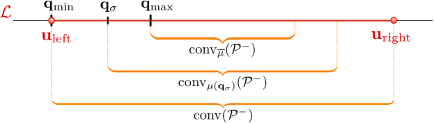
Figure 4: The second point class ${\cal P}^{-}=\{\mathbf{u}_{\mathop{{\rm left}}},\mathbf{u}_{\mathop{{\rm right}}}\}$, arranged on the line ${\cal L}$. The reduced convex hulls are indicated for the three values $\overline{\mu}\leq\mu({\mathbf{q}_{\sigma}})\leq 1$ of the regularization parameter $\mu$.

Lemma 11.

Let $\mathbf{q}$ be any point on the line ${\cal L}$ satisfying $q_{\min}\leq q_{d}\leq q_{\max}$, and define

$$\mu(\mathbf{q}):=1-\frac{(q_{d}-q_{\min})(1-\overline{\mu})}{q_{\max}-q_{\min}}~{}.$$ (38)

Then $\mu(q)\geq\overline{\mu}$, and the reduced convex hull of ${\cal P}^{-}$ is exactly equal to the following non-empty line segment of ${\cal L}$:

$$\textstyle\mathop{{\rm conv}}_{\mu(\mathbf{q})}({\cal P}^{-})=\left[\mathbf{q},\mathbf{u}_{\mathop{{\rm left}}}+\mathbf{u}_{\mathop{{\rm right}}}-\mathbf{q}\right]\subseteq\left\{\mathbf{x}\in{\cal L}\,\vphantom{x_{d}\geq q_{d}}\right.\left|\vphantom{\mathbf{x}\in{\cal L}}\,x_{d}\geq q_{d}\right\}.$$

Proof.

For arbitrary two points ${\cal P}^{-}=\{\mathbf{u}_{\mathop{{\rm left}}},\mathbf{u}_{\mathop{{\rm right}}}\}$, it is easy to see that the reduced convex hull for any reduction factor $1\geq\mu\geq\frac{1}{2}$ is given by the line segment $[\mu\mathbf{u}_{\mathop{{\rm left}}}+(1-\mu)\mathbf{u}_{\mathop{{\rm right}}},\ \mu\mathbf{u}_{\mathop{{\rm right}}}+(1-\mu)\mathbf{u}_{\mathop{{\rm left}}}]$. In our case, as $\mathbf{u}_{\mathop{{\rm left}}},\mathbf{u}_{\mathop{{\rm right}}}\in{\cal L}$, we are only interested in the $d$-th coordinate, and the calculation is slightly simplified if we write $\lambda:=\frac{1-\overline{\mu}}{q_{\max}-q_{\min}}$. We calculate the $d$-th coordinate of the left endpoint of the interval as

$$\mu(\mathbf{q})u_{\mathop{{\rm left}},d}+(1-\mu(\mathbf{q}))u_{\mathop{{\rm right}},d}=(1-(q_{d}-q_{\min})\lambda)q_{\min}+(q_{d}-q_{\min})\lambda\left(q_{\min}+\frac{1}{\lambda}\right)=q_{d},$$

and the right endpoint as

$$\mu(\mathbf{q})u_{\mathop{{\rm right}},d}+(1-\mu(\mathbf{q}))u_{\mathop{{\rm left}},d} = (1-(q_{d}-q_{\min})\lambda)\left(q_{\min}+\frac{1}{\lambda}\right)+(q_{d}-q_{\min})\lambda\,q_{\min}$$

$$= q_{\min}+\frac{1}{\lambda}+q_{\min}-q_{d}=u_{\mathop{{\rm right}},d}+u_{\mathop{{\rm left}},d}-q_{d}.$$

This proves our claim that

$$\textstyle\mathop{{\rm conv}}_{\mu(\mathbf{q})}({\cal P}^{-})=\left[\mathbf{q},\mathbf{u}_{\mathop{{\rm left}}}+\mathbf{u}_{\mathop{{\rm right}}}-\mathbf{q}\right]\subseteq\left\{\mathbf{x}\in{\cal L}\,\vphantom{x_{d}\geq q_{d}}\right.\left|\vphantom{\mathbf{x}\in{\cal L}}\,x_{d}\geq q_{d}\right\},$$

where inclusion in the line ${\cal L}$ is clear as all points are part of ${\cal L}$. However it remains to show that this interval is non-empty and lies on the right-hand side of $q$, or formally that $u_{\mathop{{\rm right}},d}+u_{\mathop{{\rm left}},d}-q_{d}\geq q_{d}$. Equivalently, the length of the interval is $u_{\mathop{{\rm right}},d}+u_{\mathop{{\rm left}},d}-q_{d}-q_{d}=\frac{q_{\max}-q_{\min}}{1-\overline{\mu}}-2(q_{d}-q_{\min})\geq 0$. Here the non-negativity follows from $1>\overline{\mu}\geq\frac{1}{2}$, so $\frac{1}{1-\overline{\mu}}\geq 2$, and $q_{d}\leq q_{\max}$ by the definition of $q_{\max}$. ∎

4.7.2 All Subsets of Support Vectors Do Appear Along the Path

Note that for any $\sigma\in\{-1,1\}^{d}$ such that $\sigma_{d-1}=\sigma_{d}=1$, we have now computed a distinct regularization value $\mu({\mathbf{q}_{\sigma}})$. We can now state the final theorem that for this parameter value, the same optimal solutions as in the optimality Theorem 8 are also optimal for the SVM distance problem (4), meaning that they realize the shortest distance between the two reduced convex hulls $\mathop{{\rm conv}}_{\mu({\mathbf{q}_{\sigma}})}({\cal P}^{+})$ and $\mathop{{\rm conv}}_{\mu({\mathbf{q}_{\sigma}})}({\cal P}^{-})$:

Theorem 12.

For every $\sigma\in\{-1,1\}^{d}$ such that $\sigma_{d-1}=\sigma_{d}=1$, let ${\mathbf{q}_{\sigma}}$ and ${\mathbf{p}_{\sigma}^{(\ell)}}$ be as defined in (18) and (19). Then for sufficiently small $\ell:=1/L>0$, the following two statements hold.

• The pair $({\mathbf{p}_{\sigma}^{(\ell)}},{\mathbf{q}_{\sigma}})$ is the unique optimal solution of the SVM optimization problem (4), which is

  $$\begin{array}[]{ll}\mathop{{\rm minimize}}_{\mathbf{p},\mathbf{q}}&\|\mathbf{p}-\mathbf{q}\|^{2}\\ \mathop{{\rm subject~{}to}}&\mathbf{p}\in\mathop{{\rm conv}}_{\mu({\mathbf{q}_{\sigma}})}\left({\cal P}^{+}\right)\\ &\mathbf{q}\in\mathop{{\rm conv}}_{\mu({\mathbf{q}_{\sigma}})}\left({\cal P}^{-}\right).\end{array}$$ (39)

• When considering the optimal solution to the dual SVM problem (3) for the regularization parameter value $\mu({\mathbf{q}_{\sigma}})$, the support vectors corresponding to the first point class ${\cal P}^{+}$ are uniquely determined, and given by the $d$ vectors

  $$\left\{\mathbf{w}_{(k,\sigma_{k})}(L)\,\vphantom{k\in\{1,\dots,d\}}\right.\left|\vphantom{\mathbf{w}_{(k,\sigma_{k})}(L)}\,k\in\{1,\dots,d\}\right\}\ ,$$

  which is a different set for every single one of the $2^{d}/4$ many possible $\sigma$.

Proof.

(i) By definition of the parameter $\mu({\mathbf{q}_{\sigma}})$, we have that

$$\textstyle{\mathbf{p}_{\sigma}^{(\ell)}}\in\mathop{{\rm conv}}_{\mu({\mathbf{q}_{\sigma}})}({\cal P}^{+})\subseteq\mathop{{\rm conv}}({\cal P}^{+})=\mathrm{Gol}^{\triangle}_{d}(L)$$

and from the previous Lemma 11 we know that

$$\textstyle{\mathbf{q}_{\sigma}}\in\mathop{{\rm conv}}_{\mu({\mathbf{q}_{\sigma}})}({\cal P}^{-})=\left[{\mathbf{q}_{\sigma}},\mathbf{u}_{\mathop{{\rm right}}}-{\mathbf{q}_{\sigma}}\right]\subseteq\left\{\mathbf{x}\in{\cal L}\,\vphantom{x_{d}\geq q_{\sigma,d}}\right.\left|\vphantom{\mathbf{x}\in{\cal L}}\,x_{d}\geq q_{\sigma,d}\right\}.$$

In other words the two feasible sets $\mathop{{\rm conv}}_{\mu({\mathbf{q}_{\sigma}})}({\cal P}^{+})$, $\mathop{{\rm conv}}_{\mu({\mathbf{q}_{\sigma}})}({\cal P}^{-})$ of the problem (39) are subsets of the feasible sets of the “artificial” distance problem (20), and the objective functions are the same. Also, we see that our pair of points $({\mathbf{p}_{\sigma}^{(\ell)}},{\mathbf{q}_{\sigma}})$ is feasible for both (20), but also the more restricted problem (39). Therefore $({\mathbf{p}_{\sigma}^{(\ell)}},{\mathbf{q}_{\sigma}})$ must be also optimal for the reduced hull problem (39), as Theorem 8 tells us that it is already optimal for (20).

For (ii), we apply the “support vector” Lemma 10 for ${\mathbf{p}_{\sigma}^{(\ell)}}$ to get uniqueness. Optimality for (3) follows from the first part which showed that ${\mathbf{p}_{\sigma}^{(\ell)}}$ is optimal for the equivalent primal problem (39). ∎

We have therefore established that exponentially many subsets of exactly $d$ support vectors out of $2d$ many input points occur as the regularization parameter $\mu$ changes between $1$ and $\overline{\mu}$. The exact number of distinct sets is $\frac{2^{d}}{4}$ when $d$ is the dimension of the space holding the input points, or $\frac{2^{n/2}}{8}$ if we express this complexity in the number of input points $n=n_{+}+n_{-}=2d+2$.

This also yields the same exponential lower bound for the number of bends in the solution path for $\mu\in[\overline{\mu},1]$, due to the following:

Lemma 13.

Let ${\mathbf{p}_{\sigma}^{(\ell)}}$ and $\mathbf{p}_{\sigma^{\prime}}^{(\ell)}$ with $\sigma\neq\sigma^{\prime}$ be two points on the solution path (restricted to the first point class). Then the path has a bend between ${\mathbf{p}_{\sigma}^{(\ell)}}$ and $\mathbf{p}_{\sigma^{\prime}}^{(\ell)}$.

Proof.

Suppose that the solution path includes the straight line segment connecting ${\mathbf{p}_{\sigma}^{(\ell)}}$ and $\mathbf{p}_{\sigma^{\prime}}^{(\ell)}$ (which are different by Corollary 9). Let $\mathbf{x}$ be some point in the relative interior of that line segment. Then it follows from Theorem 8(i) that

$$\mathbf{v}_{\tau}(\ell)^{T}\mathbf{x}<1$$

for all $\tau$ which means that $\mathbf{x}$ is not on the boundary of $\mathrm{Gol}^{\triangle}_{d}(L)$, a contradiction to $\mathbf{x}$ being on the solution path. ∎

5 Experiments

We have implemented the above Goldfarb cube construction using exact arithmetic, and could confirm the theoretical findings. We constructed the stretched dual of the Goldfarb cube $\mathrm{Gol}_{d}$ using Polymake by [17]. Figure 5 shows the two dimensional intersection of the dual Goldfarb cube $\mathrm{Gol}^{\triangle}_{d}$ with the plane $\SS$.

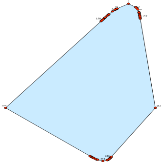
Figure 5: Example for $d=8$: The perturbed cross-polytope $\mathrm{Gol}^{\triangle}_{8}$ on 16 vertices intersected with the two dimensional plane $\SS$ has 256 vertices. Used command sequence in Polymake: Goldfarb gfarb.poly 8 1/3 1/12; center gcenter.poly gfarb.poly; polarize gpolar.poly gcenter.poly; intersection gint.poly gpolar.poly plane.poly; polymake gint.poly.

Having obtained the vertices $\{\mathbf{w}_{(k,s)}:1\leq k\leq d,~{}s\in\{-1,1\}\}$ of the polytope $\mathrm{Gol}^{\triangle}_{d}$ directly from Polymake, we then used the exact (rational arithmetic) quadratic programming solver of CGAL [1] to calculate the optimal distance vectors between the polytopes $\mathop{{\rm conv}}_{\mu}({\cal P}^{+})\subseteq\mathrm{Gol}^{\triangle}_{d}(L)$ and $\mathop{{\rm conv}}_{\mu}({\cal P}^{-})$ for some discrete values of the parameter $\mu$. Here we just manually set the stretching factor as $L:=20^{\prime}000$, and varied $\mu$ on a discrete grid within $[0.8,1]$.

For $d\leq 8$, in all cases we obtained strictly more than our lower bound of $\frac{2^{d}}{4}=\frac{1}{4}2^{\frac{n_{+}}{2}}$ bends in the path. We only counted a bend when the set of support vectors strictly changed when going from one discrete $\mu$ value to the next.

Note that it makes sense that the path complexity can be even higher than guaranteed by our lower bound from Theorem 12. This is because in our construction, we have only considered the exponentially many original facets of the point class $\mathop{{\rm conv}}({\cal P}^{+})$, and none of the additional reduced facets of the reduced convex hull $\mathop{{\rm conv}}_{\mu}({\cal P}^{+})$ that occur when some of the coordinates $\alpha_{p}$ attain their upper bounds $\alpha_{p}\leq\mu$ with equality, as the parameter $\mu$ becomes smaller.

6 Conclusion

We have shown that the worst case complexity of the solution path for SVMs — as representing one type of parameterized quadratic programs — is exponential both in the number of points $n$ and the dimension $d$. The example also shows that exponentially many (both in $n$ and $d$) distinct subsets of support vectors of the optimal solution occur as the regularization parameter changes.

We want to point out that our construction can also be interpreted as a general result in the theory of parameterized quadratic programs. Ignoring the fact that we constructed an SVM instance, we have shown that the idea of solving parameterized quadratic programs by tracking the solution path leads to an exponential-time algorithm in the worst case.

Our result also implies that the complexity of the exact solution paths is quite different from the complexity of a path of approximate solutions (of some prescribed approximation quality). For the SVM with $\ell_{2}$-loss, [18, 27] have shown that the complexity of such an approximate path is a constant depending only on the approximation quality. It is thus independent of $n$ and $d$, for all inputs, which is in very strong contrast to the worst-case complexity of the exact path as we proved here.

Acknowledgements.

This project has been supported by the Swiss National Science Foundation (SNF Project 20PA21-121957). Most of this work was done while M. Jaggi was at ETH Zurich, and C. Maria was visiting ETH Zurich. We would like to thank the anonymous reviewers for helpful comments and suggestions. We thank Joachim Giesen and Madhusudan Manjunath for stimulating discussions.

References

- [1] CGAL, Computational Geometry Algorithms Library. http://www.cgal.org.
- [2] Nina Amenta and Günter M Ziegler. Deformed Products and Maximal Shadows of Polytopes. Collection, 1996.
- [3] Francis Bach, David Heckerman, and Eric Horvitz. Considering Cost Asymmetry in Learning Classifiers. The Journal of Machine Learning Research, 7:1713–1741, 2006.
- [4] B Bank, J Guddat, D Klatte, B Kummer, and K Tammer. Non-linear parametric optimization. Birkhäuser, Basel; Boston, 1983.
- [5] Kristin P Bennett and Erin J Bredensteiner. Duality and geometry in SVM classifiers. ICML ’00: Proceedings of the 17nd International Conference on Machine Learning, 2000.
- [6] Marshall Bern and David Eppstein. Optimization over zonotopes and training support vector machines. Workshop on Algorithms and Data Structures, 2001.
- [7] Karl Heinz Borgwardt. The simplex method: a probabilistic analysis. Springer, 1987.
- [8] Christopher Burges. A Tutorial on Support Vector Machines for Pattern Recognition. Data Mining and Knowledge Discovery, 2(2):121–167, 1998.
- [9] Chih-Chung Chang and Chih-Jen Lin. Training -Support Vector Classifiers: Theory and Algorithms. Neural Computation, 13:2119–2147, 2001.
- [10] Pai-Hsuen Chen, Chih-Jen Lin, and Bernhard Schölkopf. A tutorial on -support vector machines. Applied Stochastic Models in Business and Industry, 21(2):111–136, 2005.
- [11] David J Crisp and Christopher J C Burges. A Geometric Interpretation of -SVM Classifiers. NIPS ’00: Advances in Neural Information Processing Systems 12, 2000.
- [12] Bradley Efron, Trevor Hastie, Iain Johnstone, and Robert Tibshirani. Least angle regression. Annals of Statistics, 32(2):407–499, 2004.
- [13] Mario A T Figueiredo, Robert D Nowak, and Stephen J Wright. Gradient Projection for Sparse Reconstruction: Application to Compressed Sensing and Other Inverse Problems. IEEE Journal of Selected Topics in Signal Processing, 1(4):586–597, 2007.
- [14] Carlos García, David Prett, and Manfred Morari. Model predictive control: Theory and practice - A survey. Automatica, 25(3):335–348, 1989.
- [15] Bernd Gärtner, Joachim Giesen, Martin Jaggi, and Torsten Welsch. A Combinatorial Algorithm to Compute Regularization Paths. arXiv.org, cs.LG, 2009.
- [16] Saul Gass and Thomas Saaty. The computational algorithm for the parametric objective function. Naval Research Logistics Quarterly, 2(1-2):39–45, 1955.
- [17] Ewgenij Gawrilow and Michael Joswig. Geometric Reasoning with polymake. arXiv, math.CO, 2005.
- [18] Joachim Giesen, Martin Jaggi, and Sören Laue. Approximating Parameterized Convex Optimization Problems. In Algorithms – ESA 2010, LNCS, pages 524–535. 2010.
- [19] Joachim Giesen, Jens Müller, Soeren Laue, and Sascha Swiercy. Approximating Concavely Parameterized Optimization Problems. In NIPS 2012: Advances in Neural Information Processing Systems 25, to appear, 2012.
- [20] Donald Goldfarb. Worst case complexity of the shadow vertex simplex algorithm. Technical report, Columbia University, 1983.
- [21] Donald Goldfarb. On the Complexity of the Simplex Method. In Advances in optimization and numerical analysis, Proc. 6th Workshop on Optimization and Numerical Analysis, January 1992, pages 25–38, Oaxaca, Mexico, 1994.
- [22] Ben Goodrich, David Albrecht, and Peter Tischer. Algorithms for the Computation of Reduced Convex Hulls. In AI 2009: Advances in Artificial Intelligence, pages 230–239. 2009.
- [23] Bin Gu, Jian-Dong Wang, Guan-Sheng Zheng, and Yue-Cheng Yu. Regularization Path for -Support Vector Classification. IEEE Transactions on Neural Networks and Learning Systems, 23(5):800–811, 2012.
- [24] Lacey Gunter and Ji Zhu. Computing the Solution Path for the Regularized Support Vector Regression. NIPS ’05: Advances in Neural Information Processing Systems 18, 2005.
- [25] Arash Hassibi, Jonathan How, and Stephen P Boyd. A path-following method for solving BMI problems in control. In American Control Conference, pages 1385–1389 vol.2. IEEE, 1999.
- [26] Trevor Hastie, Saharon Rosset, Robert Tibshirani, and Ji Zhu. The Entire Regularization Path for the Support Vector Machine. The Journal of Machine Learning Research, 5:1391–1415, 2004.
- [27] Martin Jaggi. Sparse Convex Optimization Methods for Machine Learning. PhD thesis, ETH Zürich, 2011.
- [28] Seung-Jean Kim, K Koh, M Lustig, Stephen P Boyd, and D Gorinevsky. An Interior-Point Method for Large-Scale l1-Regularized Least Squares. Selected Topics in Signal Processing, IEEE Journal of, 1(4):606–617, 2007.
- [29] Gyemin Lee and Clayton D Scott. The One Class Support Vector Machine Solution Path. ICASSP 2007. IEEE International Conference on Acoustics, Speech and Signal Processing, 2:II–521 – II–524, 2007.
- [30] Yoonkyung Lee and Zhenhuan Cui. Characterizing the solution path of multicategory support vector machines. Statistica Sinica, 2006.
- [31] Gaëlle Loosli, Gilles Gasso, and Stéphane Canu. Regularization Paths for -SVM and -SVR. ISNN, International Symposium on Neural Networks, LNCS, 4493:486, 2007.
- [32] Julien Mairal and Bin Yu. Complexity Analysis of the Lasso Regularization Path. In ICML 2012: Proceedings of the 29th International Conference on Machine Learning, May 2012.
- [33] Dmitry M Malioutov, Müjdat Cetin, and Alan S Willsky. Homotopy continuation for sparse signal representation. In ICASSP ’05 - IEEE International Conference on Acoustics, Speech, and Signal Processing, pages 733–736 Vol. 5, 2005.
- [34] Harry Markowitz. Portfolio Selection. The Journal of Finance, 7(1):77–91, 1952.
- [35] Katta G Murty. Linear Complementarity, Linear and Nonlinear Programming. University of Michigan, 1988.
- [36] Chong-Jin Ong, Shiyun Shao, and Jianbo Yang. An Improved Algorithm for the Solution of the Regularization Path of Support Vector Machine. IEEE Transactions on Neural Networks, 21(3):451–462, 2010.
- [37] Michael R Osborne. An effective method for computing regression quantiles. IMA Journal of Numerical Analysis, 12(2):151–166, 1992.
- [38] Michael R Osborne, Brett Presnell, and Berwin A Turlach. A new approach to variable selection in least squares problems. IMA Journal of Numerical Analysis, 20(3):389–403, 2000.
- [39] Anthony L Peressini, Francis E Sullivan, and J Jerry Uhl. The mathematics of nonlinear programming. Undergraduate texts in mathematics. Springer-Verlag, 1988.
- [40] Klaus Ritter. Ein Verfahren zur Lösung parameter-abhängiger, nicht-linearer Maximum-Probleme. Unternehmensforschung, 6:149–166, 1962.
- [41] Klaus Ritter. On Parametric Linear and Quadratic Programming Problems. Mathematical Programming: Proceedings of the International Congress on Mathematical Programming. Rio de Janeiro, 6-8 April, 1981 / ed.: R. W. Cottle, M. L. Kelmanson, B. H. Korte, pages 307–335, 1984.
- [42] Saharon Rosset and Ji Zhu. Piecewise linear regularized solution paths. The Annals of Statistics, 35(3):1012–1030, 2007.
- [43] Bernhard Schölkopf, Joachim Giesen, and Simon Spalinger. Kernel Methods for Implicit Surface Modeling. In NIPS ’04: Advances in Neural Information Processing Systems 17, 2004.
- [44] Alex J Smola and Bernhard Schölkopf. A tutorial on support vector regression. Statistics and Computing, 14:199–222, 2004.
- [45] Robert Tibshirani. Regression Shrinkage and Selection via the Lasso. Journal of the Royal Statistical Society. Series B (Methodological), pages 267–288, 1996.
- [46] Ivor W Tsang, James T Kwok, and Pak-Ming Cheung. Core Vector Machines: Fast SVM Training on Very Large Data Sets. Journal of Machine Learning Research, 6:363–392, 2005.
- [47] Gang Wang. A New Solution Path Algorithm in Support Vector Regression. IEEE Transactions on Neural Networks, 2008.
- [48] Gang Wang, Tao Chen, Dit-Yan Yeung, and Frederick H Lochovsky. Solution Path for Semi-Supervised Classification with Manifold Regularization. ICDM ’06: Sixth International Conference on Data Mining, pages 1124–1129, 2006.
- [49] Gang Wang, Dit-Yan Yeung, and Frederick H Lochovsky. Two-dimensional solution path for support vector regression. ICML ’06: Proceedings of the 23rd International Conference on Machine Learning, pages 993–1000, 2006.
- [50] Gang Wang, Dit-Yan Yeung, and Frederick H Lochovsky. A kernel path algorithm for support vector machines. ICML ’07: Proceedings of the 24th International Conference on Machine Learning, 2007.
- [51] Gang Wang, DY Yeung, and Frederick H Lochovsky. The Kernel Path in Kernelized LASSO. International Conference on Artificial Intelligence and Statistics, 2007.
- [52] Zhi-li Wu, Aijun Zhang, Chun-hung Li, and Agus Sudjianto. Trace Solution Paths for SVMs via Parametric Quadratic Programming. KDD ’08 DMMT Workshop, 2008.
- [53] Günter M Ziegler. Lectures on Polytopes, volume 152 of Graduate Texts in Mathematics. Springer Verlag, 1995.