A partial fraction decomposition of the Fermi function

Abstract

A partial fraction decomposition of the Fermi function resulting in a finite sum over simple poles is proposed. This allows for efficient calculations involving the Fermi function in various contexts of electronic structure or electron transport theories. The proposed decomposition converges in a well-defined region faster than exponential and is thus superior to the standard Matsubara expansion.

1 Introduction

Many problems in electronic structure and electron transport calculations involve the evaluation of integrals containing the Fermi function. These are in general difficult to compute and therefore several approximation schemes have been developed [1, 2, 3, 4, 5, 6]. Among them the Sommerfeld expansion [1] and the Matsubara expansion [2] being the most prominent ones. While the former is by construction useful for low temperatures, the latter provides in principle a way to cover the range from low to high temperatures. Moreover, it turns out that the expansion in a (finite) sum of simple poles is particularly suitable for evaluating the integrals by making use of the residue theorem. For example, finite temperature charge density calculations only require the evaluation of a Green’s function at a finite set of energies [7, 8] given by the poles of the expansion. Recently the same concept was used for the auxiliary density matrix propagation in the context of time-resolved electron transport in molecular wires [9]. The major disadvantage of the Matsubara expansion consists in its poor convergence behavior, the error decreasing only linearly with the number of terms in the expansion. Here we derive an expansion of the Fermi function in terms of simple poles with particularly simple coefficients. We will show that it converges very rapidly with increasing order of the expansion in a well-defined region which is found to increase linearly with the order.

For the following discussion it is convenient to write the Fermi function $f(\varepsilon)$ in terms of a dimensionless variable $x$,

$$f(x)=\frac{1}{1+e^{x}}\quad\mbox{with}\quad x=\frac{\varepsilon-\mu}{kT}\;,$$ (1)

where $\mu$ is the chemical potential, $T$ is the temperature, $k$ is the Boltzmann factor and $\varepsilon$ denotes the energy. The expansion consists in finding a partial fraction decomposition with simple poles of the form

$$f(x)=\frac{1}{2}-\sum_{p=-\infty}^{\infty}\frac{A_{p}}{x-x_{p}}\;,$$ (2)

where $A_{p}$ are expansion coefficients and $x_{p}$ are (possibly complex) poles. For practical purposes the sum over $p$ is truncated and the Fermi function is approximated by $f(x)\approx f_{N}(x)$ with $N$ being the number of terms in the expansion.

For example, the well-known Matsubara expansion [2] is given in terms of the purely imaginary zeros $x_{n}$ of the denominator in Eq. (1), $x_{p}=\imath\pi(2p{-}1)$, which yields coefficients $A_{p}=1$ and gives

$$f_{N}(x)=\frac{1}{2}-\sum_{p=1}^{N}\left(\frac{1}{x+\imath\pi(2p{-}1)}+\frac{1}{x-\imath\pi(2p{-}1)}\right)\;.$$ (3)

For $N\rightarrow\infty$ in Eq. (3) the expansion becomes exact. However, the convergence is very slow, which renders the application of this expansion impractical especially for low temperatures.

2 Partial Fraction Decomposition

The proposed partial fraction decomposition (PFD) is obtained by firstly writing Eq. (1) as [5]

$$f(x)=\frac{1}{2}-\frac{1}{2}\tanh(x/2)=\frac{1}{2}-\frac{\sinh(x/2)}{2\cosh(x/2)}\;,$$ (4)

and secondly by expanding numerator and denominator in a power series, truncating the respective sums, such that the degree of the polynomial in the denominator is larger than the degree of the numerator polynomial. This procedure gives

$$f_{N}(x)=\frac{1}{2}-\frac{1}{2}\frac{P_{N{-}1}(x/2)}{Q_{N}(x/2)}\;,$$ (5)

with polynomials

$$P_{N}(x)=\sum\limits_{m=0}^{N}\frac{x^{2m+1}}{(2m{+}1)!}\qquad\mbox{and}\qquad Q_{N}(x)=\sum\limits_{m=0}^{N}\frac{x^{2m}}{(2m)!}\;.$$ (6)

This construction allows for a PFD, i. e. an expansion of the form

$$\frac{P_{N{-}1}(x/2)}{Q_{N}(x/2)}=\sum_{p=1}^{N}\left(\frac{A_{p}}{x/2-x_{p}}+\frac{B_{p}}{x/2+x_{p}}\right).$$ (7)

Here, $\pm x_{p}$ are the zeros of the polynomial $Q_{N}$, which appear in pairs since $Q_{N}$ contains only even powers of $x/2$. It can be shown that the zeros can be obtained as $x_{p}=\sqrt{z_{p}}$, whereby the $z_{p}$ are the eigenvalues of the following matrix [5],

$$Z_{ij}=2i(2i{-}1)\delta_{j,i+1}-2N(2N{-}1)\delta_{iN},\quad i,j=1,\ldots,N.$$ (8)

The eigenvalues can be efficiently calculated using standard methods. In Fig. 1 we have plotted the poles of Eq. (7), given as $\pm 2x_{p}{=}\pm 2\sqrt{z_{p}}$, for three sets of eigenvalues $z_{p}$ for different sizes $N{\times}N$ of the matrix $Z_{ij}$. As can be seen from the figure some of the poles $\pm 2x_{p}$ arising from the PFD are purely imaginary and are close to the Matsubara poles. On the other hand there are also poles with a non-vanishing real part, which display an irregular distribution. These very poles improve considerably the approximation for the Fermi function as we show below.

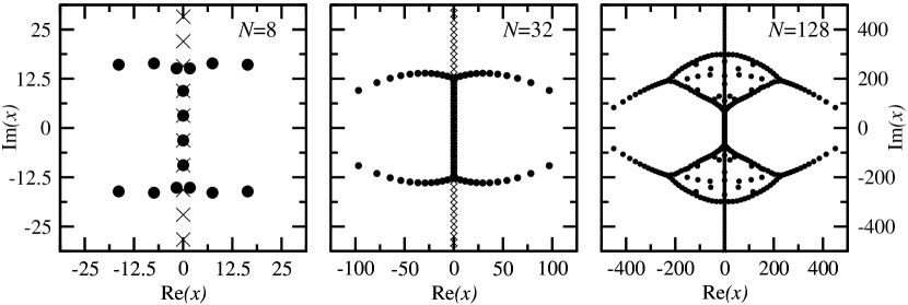
Figure 1: Poles (symbol $\bullet$) of the PFD expansion, i. e. $\pm 2\sqrt{z_{p}}$, with $z_{p}$ the eigenvalues of matrix (8) for various orders $N$. For comparison the purely imaginary poles (symbol $\times$) of the Matsubara expansion (3) are shown as well. Note the different scales of the three graphs.

It remains to determine the corresponding expansion coefficients $A_{p}$ and $B_{p}$ in Eq. (7). Multiplying both sides of this equation by $(x/2-x_{k})$ and letting $x\to 2x_{k}$ leaves on the right side of Eq. (7) only the term $A_{k}$, which is thus given as

$$A_{k}=\lim\limits_{x\to 2x_{k}}(x/2{-}x_{k})\frac{P_{N-1}(x/2)}{Q_{N}(x/2)}=\lim\limits_{\eta\to 0}\frac{\eta\>P_{N-1}(x_{k}{+}\eta)}{Q_{N}(x_{k}{+}\eta)}\;.$$ (9)

By means of the definitions (6) one finds from this limit $A_{k}\equiv 1$ and similarly $B_{k}\equiv 1$. Thus we arrive at the main result of this paper: The Fermi function can be approximated by the finite sum

$$f_{N}(x)=\frac{1}{2}-\sum_{p=1}^{N}\left(\frac{1}{x+2\sqrt{z_{p}}}+\frac{1}{x-2\sqrt{z_{p}}}\right)\;,$$ (10)

with $z_{p}$ the eigenvalues of matrix (8).

Figure 2: Approximated Fermi function $f_{N}(x)$ for expansion orders $N=2,8,32,128$ (full lines). Panel a: Matsubara expansion Eq. (3), panel b: partial fraction decomposition Eq. (10). The curves are shown for $x<0$ only and are vertically shifted by $0.2$ for better visibility. The exact Fermi function Eq. (1) is denoted by dotted lines.

The formal structure of this approximation is similar to the Matsubara expansion (3). However, taking advantage of having complex rather than purely imaginary poles makes the PFD for given order $N$ of the expansion vastly superior to the Matsubara expansion. This can be seen in Fig. 2, where we have shown both expansions for different orders $N$. Whereas the Matsubara expansion (3) in Fig. 2a does not give a reasonable representation for any of the orders shown, the PFD expansion (10) in Fig. 2b improves rapidly with increasing order.

3 Convergence properties

From Fig. 2 it becomes clear that the PFD is indeed converging faster than the Matsubara expansion. In the following we will quantify the rate of convergence as $N\rightarrow\infty$ and give a range for $x$ where this convergence behavior can be expected. To this end we define the deviation of the finite expansion from the exact function as

$$\delta f_{N}(x)=f(x)-f_{N}(x).$$ (11)

Regarding the PFD one makes two observations: First, in terms of the scaled variable $y=x/4N$ one finds in the limit of large $N$,

$$\lim_{N\to\infty}\delta f_{N}(x{=}y4N)=\left\{\begin{array}[]{llll}0&&\mbox{for}&\frac{x}{4N}{=}y\geq-1\\ \frac{1}{2}\left(1+\frac{4N}{x}\right)=\frac{1}{2}\left(1+\frac{1}{y}\right)&&\mbox{for}&\frac{x}{4N}{=}y\leq-1\\ \end{array}\right.$$ (12)

The asymptotic function (12) is shown along with deviations $\delta f_{N}(y)$ for various finite $N$ in Fig. 3a. Second, in the range $-4N\leq x$, i. e. $-1<y$, the rate of convergence is given by the asymptotic expression

$$\delta f_{N}(x{=}y4N)\approx\frac{(x/2)^{2N}}{(2N)!}=\frac{(y2N)^{2N}}{(2N)!},$$ (13)

which due to the factorial in the denominator decreases faster than exponential. Eqs. (12) and (13) are the main results of this section. They corroborate the statement that the PFD is expected to yield a better convergence and allow to estimate the error in actual calculations.

Figure 3: Deviation $\delta f_{N}$ of the approximated Fermi function form the exact one as defined in Eq. (11). Left panel: $\delta f_{N}$ as a function of the scaled argument $y=x/4N$ for $N=2,\>8,\>32,\>128$ (solid lines) and the asymptotic expression (dashed line) as given by Eq. (12). The dotted line shows $\delta f_{128}$ for the Matsubara expansion. Right panel:$\delta f_{N}$ as a function of the expansion order $N$ for three arguments $x=-5,\>-25,\>-125$. We compare the Matsubara expansion (dotted lines) and PFD (solid lines). For the latter case we show also the asymptotic behavior according to Eq. (13) by dashed lines.

In the remaining part of this section we will justify and discuss Eqs. (12) and (13). Considering the case $y<-1$, one finds from Eq. (10), that a finite expansion behaves as $f_{N}(x)\propto 1/x$ for $x\to-\infty$. Since the Fermi function gives $f(x)=1$ for $x\to-\infty$ one expects qualitatively the behavior given in Eq. (12). This holds true for any expansion resulting in a finite sum over simple poles including the Matsubara expansion, which is shown for $N=128$ as dotted line in Fig. 3a. In order to verify that this behavior is indeed restricted to $y<-1$, or equivalently to $x\leq-4N$, we write the polynomial $Q_{N}$ from Eq. (6) explicitly as

$$Q_{N}(x/2)=Q_{N}(y2N)=\sum\limits_{m=0}^{N}q_{mN}(y)\qquad\mbox{with}\quad q_{mN}(y)=\frac{(2N)^{2m}}{(2m)!}y^{2m}.$$ (14)

Assuming $y<-1$, we see that the ratio of two successive terms

$$\frac{q_{m\,N}(y)}{q_{m-1\,N}(y)}=y^{2}\frac{(2N)^{2}}{2m(2m{-}1)}$$ (15)

is always larger than $1$; the terms are monotonically increasing. Thus terms with $m\gg 1$ dominate the sum and we replace the coefficients in $q_{mN}$ by the coefficient from $q_{NN}$, i.e. instead of the sum (14) we define

$$\tilde{Q}_{N}(y2N)=\sum\limits_{m=0}^{N}\tilde{q}_{mN}(y)\qquad\mbox{with}\quad\tilde{q}_{mN}(y)=\frac{(2N)^{2N}}{(2N)!}y^{2m}.$$ (16)

It turns out that in the limit $N\to\infty$ this sum becomes equal to $Q_{N}(y2N)$, which can be seen by considering the difference of the newly defined terms in Eq. (16) from the original terms in Eq. (14). For $m=N-n$ one gets

$$1-\frac{q_{N-n,N}(y)}{\tilde{q}_{N-n,N}(y)}=1-(2N)^{-2n}\frac{(2N)!}{(2N{-}2n)!}=\frac{n/2{-}n^{2}}{N}+{\cal O}\left(\frac{1}{N^{2}}\right).$$ (17)

This expression vanishes for $n=0$ and can be made arbitrarily small by increasing $N$ for all $n\ll N$. Terms with larger $n$ can be neglected because they are exponentially small compared to those with smaller $n$. Since the sum (16) is a geometric series we obtain

$$Q_{N}(y2N)=\tilde{Q}_{N}(y2N)=\frac{y^{2}}{y^{2}{-}1}\>q_{NN}(y)\qquad\mbox{for}\quad N\to\infty.$$ (18)

Analogous considerations for the other polynomial from Eqs. (6) yield

$$P_{N{-}1}(y2N)\approx\frac{(2N)^{2N{-}1}}{(2N{-}1)!}\>\frac{y^{2N+1}}{y^{2}-1}=\frac{y^{2}}{y^{2}{-}1}\>p_{N-1,N}(y)$$ (19)

with $p_{mN}(y)=(y2N)^{2m+1}/(2m{+}1)!$ and we get as an approximation for the ratio, once again using $N\gg 1$,

$$\frac{P_{N{-}1}(y2N)}{Q_{N}(y2N)}\approx\frac{1}{y}=\frac{4N}{x},$$ (20)

which explains the asymptotic behavior of $\delta f_{N}(x)$ in Eq. (12) for $x<-4N$.

Turning now to the case $y>-1$, we firstly note that there is a crossover for the ratio (15) at $|y|N$; whereas for $m<|y|N$ the terms are increasing, they decrease for $m>|y|N$. Thus, for large $N$ the polynomial expression (5) converges to the exact expression (4) and the deviation $\delta f_{N}(x)$ vanishes as given by Eq. (12) for $x>-4N$. In order to quantify the rate of convergence it is useful to define complementary sums to $P_{N}$ and $Q_{N}$, namely

$$\bar{P}_{N}(x)=\sum\limits_{m=N{+}1}^{\infty}\frac{x^{2m+1}}{(2m{+}1)!}\qquad\mbox{and}\qquad\bar{Q}_{N}(x)=\sum\limits_{m=N{+}1}^{\infty}\frac{x^{2m}}{(2m)!}\;.$$ (21)

Therewith the deviation reads

$$\delta f_{N}(y4N) = \frac{\sinh(y2N)-\bar{P}_{N{-}1}(y2N)}{2\cosh(y2N)-2\bar{Q}_{N}(y2N)}-\frac{\sinh(y2N)}{2\cosh(y2N)}$$ (22)

$$\approx e^{-y2N}\left(\bar{Q}_{N}(y2N)-\bar{P}_{N{-}1}(y2N)\right)\;.$$

The approximation in the second line applies to large values of $N$. We can choose, for any given $y<0$, $N$ sufficiently large such that $\exp(-y2N){\gg}\exp(+y2N)$. The infinite sums defined in (21) become small compared to the exponentials, $\bar{Q}_{N}(y2N){\ll}1{\ll}\exp(-y2N)$ and $\bar{P}_{N{-}1}(y2N){\ll}1{\ll}\exp(-y2N)$. It remains to estimate their behavior for large $N$ which can be done in analogy to the considerations for $Q_{N}$ and $P_{N}$, cf. Eqs. (18) and (19). Here the ratio of successive terms as defined in Eq. (15) is always smaller than $1$ and the first terms in the sum can be used to estimate the sums. One gets

$$\bar{P}_{N}(y2N)\approx\frac{1}{1{-}y^{2}}p_{N,N}(y)\qquad\mbox{and}\qquad\bar{Q}_{N}(y2N)\approx\frac{1}{1{-}y^{2}}q_{N+1,N}(y).$$ (23)

This directly leads to Eq. (13) and concludes the derivation.

Fig. 3b shows this estimate along with the numerically calculated deviation $\delta f_{N}$ as a function of the expansion order $N$ for selected values of $x$. Even for small values of $N$ an overall good agreement is found. Moreover, one sees that the deviation $\delta f_{N}$ is of order $1$ as long as $N<-x/4$. However, for $N>-x/4$ (this is where the dashed lines start) it decreases very rapidly due to the factorial in the denominator in Eq. (13).

4 Conclusions

We have proposed the expansion (10) of the Fermi function (1) by using a partial fraction decomposition. Its application requires only the diagonalization of a matrix, given in Eq. (8), which has the same dimension $N$ as the expansion. The expansion converges faster than exponential with increasing order $N$ for arguments $|x|<4N$. In other words, the approximation becomes not only more accurate for higher orders, it can also be used for a wider range of arguments. An estimate for the error is explicitly given by Eq. (13). Due to the beneficial convergence properties and the straightforward implementation we expect the PFD to be of great value in any application based on an expansion of the Fermi function as sum of over simples poles. Finally, we would like to notice that an analogous expansion can be found for the Bose-Einstein distribution.

References

- [1] N. W. Ashcroft, N. D. Mermin, Solid state physics, Saunders College, 1976.
- [2] G. D. Mahan, Many Particle Physics, 2nd Edition, Plenum, New York, 1990.
- [3] S. Goedecker, Integral representation of the Fermi distribution and its applications in electronic-structure calculations, Phys. Rev. B 48 (1993) 17573.
- [4] D. M. C. Nicholson, X.-G. Zhang, Approximate occupation functions for density-functional calculations, Phys. Rev. B 56 (1997) 12805.
- [5] F. Gagel, Finite-temperature evaluation of the Fermi density operator, J. Comp. Phys. 139 (1998) 399.
- [6] T. Ozaki, Continued fraction representation of the Fermi-Dirac function for large-scale electronic structure calculations, Phys. Rev. B 75 (2007) 035123.
- [7] K. Wildberger, P. Lang, R. Zeller, P. H. Dederichs, Fermi-Dirac distribution in ab initio Green’s-function calculations, Phys. Rev. B 52 (1995) 11502.
- [8] M. J. Watrous, L. Wilets, J. J. Rehr, Green’s-function calculation of electron screening in a plasma, Phys. Rev. E 59 (1999) 3554.
- [9] S. Welack, M. Schreiber, U. Kleinekathöfer, The influence of ultrafast laser pulses on electron transfer in molecular wires studied by a non-markovian density-matrix approach, J. Chem. Phys. 124 (2006) 044712.