Technical Report # KU-EC-09-3:
A Probabilistic Characterization of Random Proximity Catch Digraphs and the Associated Tools

Abstract

Proximity catch digraphs (PCDs) are based on proximity maps which yield proximity regions and are special types of proximity graphs. PCDs are based on the relative allocation of points from two or more classes in a region of interest and have applications in various fields. In this article, we provide auxiliary tools for and various characterizations of PCDs based on their probabilistic behavior. We consider the cases in which the vertices of the PCDs come from uniform and non-uniform distributions in the region of interest. We also provide some of the newly defined proximity maps as illustrative examples.

Keywords: class cover catch digraph (CCCD); central similarity PCD; Delaunay triangulation; domination number; proportional-edge PCD; proximity graph; random graph; relative arc density

1 Introduction

The proximity catch digraphs (PCDs) are a special type of proximity graphs which are based on proximity maps and are used in disciplines where shape and structure are crucial. Examples include computer vision (dot patterns), image analysis, pattern recognition (prototype selection), geography and cartography, visual perception, biology, etc. Proximity graphs were first introduced by Toussaint, (1980), who called them relative neighborhood graphs. The notion of relative neighborhood graph has been generalized in several directions and all of these graphs are now called proximity graphs. From a mathematical and algorithmic point of view, proximity graphs fall under the category of computational geometry.

In recent years, a new classification and spatial pattern analysis approach which is based on the relative positions of the data points from various classes has been developed. Priebe et al., (2001) introduced the class cover catch digraphs (CCCDs) and gave the exact and the asymptotic distribution of the domination number of the CCCD based on two data sets $\mathcal{X}_{n}$ and $\mathcal{Y}_{m}$ both of which are random samples from uniform distribution on a compact interval in $\mathbb{R}$. DeVinney et al., (2002), Marchette and Priebe, (2003), Priebe et al., 2003b , Priebe et al., 2003a , and DeVinney and Priebe, (2006) applied the concept in higher dimensions and demonstrated relatively good performance of CCCD in classification. The employed methods involve data reduction (condensing) by using approximate minimum dominating sets as prototype sets, since finding the exact minimum dominating set is in general an NP-hard problem — in particular, for CCCD — (see DeVinney, (2003)). Furthermore, the exact and the asymptotic distribution of the domination number of the CCCDs are not analytically tractable in higher dimensions. Ceyhan, (2004) extended the concept of CCCDs by introducing PCDs, which do not suffer from some of the shortcomings of CCCDs in higher dimensions. In particular, two new types of PCDs (namely, proportional-edge and central similarity PCDs) are introduced; distribution of the domination number of proportional-edge PCDs is calculated, and is applied in testing spatial patterns of segregation and association (Ceyhan and Priebe, (2005, 2007)). The distributions of the relative arc density of these PCD families are also derived and used for the same purpose (Ceyhan et al., (2006) and Ceyhan et al., (2007)).

A general definition of proximity graphs is as follows: Let $V$ be any finite or infinite set of points in $\mathbb{R}^{d}$. Each (unordered) pair of points $(p,q)\in V\times V$ is associated with a neighborhood $\mathfrak{N}(p,q)\subseteq\mathbb{R}^{d}$. Let $\mathfrak{P}$ be a property defined on $\mathfrak{N}=\{\mathfrak{N}(p,q):\;(p,q)\in V\times V\}$. A proximity (or neighborhood) graph $G_{\mathfrak{N},\mathfrak{P}}(V,E)$ defined by the property $\mathfrak{P}$ is a graph with the set of vertices $V$ and the set of edges $E$ such that $(p,q)\in E$ iff $\mathfrak{N}(p,q)$ satisfies property $\mathfrak{P}$. Examples of most commonly used proximity graphs are the Delaunay tessellation, the boundary of the convex hull, the Gabriel graph, relative neighborhood graph, Euclidean minimum spanning tree, and sphere of influence graph of a finite data set. See, e.g., Jaromczyk and Toussaint, (1992).

The relative allocation of the data points are used to construct a proximity digraph. A digraph is a directed graph, i.e., a graph with directed edges from one vertex to another based on a binary relation. Then the pair $(p,q)\in V\times V$ is an ordered pair and $(p,q)$ is an arc (directed edge) denoted $pq$ to reflect its difference from an edge. For example, the nearest neighbor (di)graph in Paterson and Yao, (1992) is a proximity digraph. The nearest neighbor digraph, denoted $NND(V)$, has the vertex set $V$ and $pq$ an arc iff $d(p,q)=\min_{v\in V\setminus\{p\}}d(p,v)$. That is, $pq$ is an arc of $NND(V)$ iff $q$ is a nearest neighbor of $p$. Note that if $pq$ is an arc in $NND(V)$, then $(p,q)$ is an edge in $RNG(V)$. Our PCDs are based on the property $\mathfrak{P}$ that is determined by the following mapping which is defined in a more general space than $\mathbb{R}^{d}$. Let $(\Omega,\mathcal{M})$ be a measurable space. The proximity map $N(\cdot)$ is given by $N:\Omega\rightarrow\wp(\Omega)$, where $\wp(\cdot)$ is the power set functional, and the proximity region of $x\in\Omega$, denoted $N(x)$, is the image of $x\in\Omega$ under $N(\cdot)$. The points in $N(x)$ are thought of as being “closer” to $x\in\Omega$ than are the points in $\Omega\setminus N(x)$. Proximity maps are the building blocks of the proximity graphs of Toussaint, (1980); an extensive survey is available in Jaromczyk and Toussaint, (1992).

The PCD $D=(\mathcal{V},\mathcal{A})$ has the vertex set $\mathcal{V}=\bigl{\{}p_{1},p_{2},\ldots,p_{n}\bigr{\}}$ and the arc set $\mathcal{A}$ is defined by $p_{i}p_{j}\in\mathcal{A}$ iff $p_{j}\in N(p_{i})$ for $i\not=j$. Notice that $D$ depends on the proximity map $N(\cdot)$, and if $p_{j}\in N(p_{i})$, then $N(p_{i})$ is said to catch $p_{j}$. Hence the name proximity catch digraph. If arcs of the form $p_{i}p_{i}$ (i.e., loops) were allowed, $D$ would have been called a pseudodigraph according to some authors (see, e.g., Chartrand and Lesniak, (1996)).

In this article, we provide a probabilistic characterization of the proximity maps, and the associated regions and PCDs, and introduce auxiliary tools for the PCDs. We define the proximity maps and data-random PCDs in Section 2, describe the auxiliary tools (such as edge and vertex regions) for the construction of PCDs in Section 3, provide $\Gamma_{1}$-regions and the related concepts for proximity maps in Section 4, discuss the examples of proximity maps in Delaunay triangles in Section 6, and provide the transformations preserving uniformity on triangles in $\mathbb{R}^{2}$ in Section 5. We investigate the characterization of proximity regions and the associated PCDs in Section 7, introduce $\Gamma_{k}$-regions for proximity maps in $T\left(\mathcal{Y}_{3}\right)$ in Section 8, $\kappa$-values for the proximity maps in $T\left(\mathcal{Y}_{3}\right)$ in Section 9, and provide discussion and conclusions in Section 10.

2 Proximity Maps and Data-Random PCDs

Let $\mathcal{X}_{n}=\bigl{\{}X_{1},X_{2},\ldots,X_{n}\bigr{\}}$ and $\mathcal{Y}_{m}=\bigl{\{}Y_{1},Y_{2},\ldots,Y_{m}\bigr{\}}$ be two data sets from classes $\mathcal{X}$ and $\mathcal{Y}$ of $\Omega$-valued random variables whose joint pdf is $f_{X,Y}$. Let $d(\cdot,\cdot):\Omega\times\Omega\rightarrow[0,\infty)$ be a distance function. The class cover problem for a target class, say $\mathcal{X}_{n}$, refers to finding a collection of neighborhoods, $N(X_{i})$ around $X_{i}\in\mathcal{X}_{n}$ such that (i) $\mathcal{X}_{n}\subset\bigl{(}\bigcup_{i}N(X_{i})\bigr{)}$ and (ii) $\mathcal{Y}_{m}\cap\bigl{(}\bigcup_{i}N(X_{i})\bigr{)}=\emptyset$. A collection of neighborhoods satisfying both conditions is called a class cover. A cover satisfying condition (i) is a proper cover of class $\mathcal{X}$ while a collection satisfying condition (ii) is a pure cover relative to class $\mathcal{Y}$. From a practical point of view, for example for classification, of particular interest are the class covers satisfying both (i) and (ii) with the smallest collection of neighborhoods, i.e., minimum cardinality cover. This class cover problem is a generalization of the set cover problem in Garfinkel and Nemhauser, (1972) that emerged in statistical pattern recognition and machine learning, where an edited or condensed set (prototype set) is selected from $\mathcal{X}_{n}$ (see, e.g., Devroye et al., (1996)).

In particular, we construct the proximity regions using data sets from two classes. Given $\mathcal{Y}_{m}\subseteq\Omega$, the proximity map $N_{\mathcal{Y}}(\cdot)$ associates a proximity region $N_{\mathcal{Y}}(x)\subseteq\Omega$ with each point $x\in\Omega$. The region $N_{\mathcal{Y}}(x)$ is defined in terms of the distance between $x$ and $\mathcal{Y}_{m}$. More specifically, our proximity maps will be based on the relative position of points from class $\mathcal{X}$ with respect to the Delaunay tessellation of the class $\mathcal{Y}$. See Okabe et al., (2000) and Ceyhan, (2009) for more on Delaunay tessellations.

If $\mathcal{X}_{n}$ is a set of $\Omega$-valued random variables then $N_{\mathcal{Y}}(X_{i})$ are random sets. If $X_{i}$ are independent identically distributed then so are the random sets $N_{\mathcal{Y}}(X_{i})$. We define the data-random PCD $D=(\mathcal{V},\mathcal{A})$ — associated with $N_{\mathcal{Y}}(\cdot)$ — with vertex set $\mathcal{V}=\mathcal{X}_{n}$ and arc set $\mathcal{A}$ by $X_{i}X_{j}\in\mathcal{A}\iff X_{j}\in N_{\mathcal{Y}}(X_{i})$. Since this relationship is not symmetric, a digraph is needed rather than a graph. The random digraph $D$ depends on the (joint) distribution of the $X_{i}$ and on the map $N_{\mathcal{Y}}(\cdot)$.

The PCDs are closely related to the proximity graphs of Jaromczyk and Toussaint, (1992) and might be considered as a special case of covering sets of Tuza, (1994) and intersection digraphs of Sen et al., (1989). This data random proximity digraph is a vertex-random proximity digraph which is not of standard type. The randomness of the PCDs lies in the fact that the vertices are random with joint pdf $f_{X,Y}$, but arcs $X_{i}X_{j}$ are deterministic functions of the random variable $X_{j}$ and the set $N_{\mathcal{Y}}(X_{i})$.

For example, the CCCD of Priebe et al., (2001) can be viewed as an example of PCD with $N_{\mathcal{Y}}(x)=B(x,r(x))$, where $r(x):=\min_{\mathsf{y}\in\mathcal{Y}_{m}}d(x,\mathsf{y})$. The CCCD is the digraph of order $n$ with vertex set $\mathcal{X}_{n}$ and an arc from $X_{i}$ to $X_{j}$ iff $X_{j}\in B(X_{i},r(X_{i}))$. That is, there is an arc from $X_{i}$ to $X_{j}$ iff there exists an open ball centered at $X_{i}$ which is “pure” (or contains no elements) of $\mathcal{Y}_{m}$, and simultaneously contains (or “catches”) point $X_{j}$.

3 Auxiliary Tools for the Construction of PCDs in $\mathbb{R}^{d}$

Recall the proximity map (associated with CCCD) in $\mathbb{R}$ is defined as $B(x,r(x))$ where $r(x)=\min_{y\in\mathcal{Y}_{m}}d(x,y)$ with $d(x,y)$ being the Euclidean distance between $x$ and $y$ (Priebe et al., (2001)). Our goal is to extend this idea to higher dimensions and investigate the associated digraph. Now let $\mathcal{Y}_{m}=\left\{\mathsf{y}_{1},\mathsf{y}_{2},\ldots,\mathsf{y}_{m}\right\}\subset\mathbb{R}^{d}$. For $d=1$ the proximity map associated with CCCD is defined as the open ball $N_{S}(x):=B(x,r(x))$ for all $x\in\mathbb{R}\setminus\mathcal{Y}_{m}$ and for $x\in\mathcal{Y}_{m}$, define $N_{S}(x)=\{x\}$. Furthermore, dependence on $\mathcal{Y}_{m}$ is through $r(x)$. Hence $N_{S}(x)$ is based on the intervals $I_{i-1}=\left(\mathsf{y}_{(i-1):m},\mathsf{y}_{i:m}\right)$ for $i=1,2,\ldots,(m+1)$ with $\mathsf{y}_{0:m}=-\infty$ and $\mathsf{y}_{(m+1):m}=\infty$ where $\mathsf{y}_{i:m}$ is the $i^{th}$ order statistic in $\mathcal{Y}_{m}$. This intervalization can be viewed as a tessellation since it partitions $C_{H}\left(\mathcal{Y}_{m}\right)$, the convex hull of $\mathcal{Y}_{m}$. For $d>1$, a natural tessellation that partitions $C_{H}\left(\mathcal{Y}_{m}\right)$ is the Delaunay tessellation (see Okabe et al., (2000) and Ceyhan, (2009)). Let $\mathcal{T}_{i}$ for $i=1,2,\ldots,J$ be the $i^{th}$ Delaunay cell in the Delaunay tessellation of $\mathcal{Y}_{m}$. In $\mathbb{R}$, we implicitly use the cell that contains $x$ to define the proximity map.

A natural extension of the proximity region $N_{S}(x)$ to multiple dimensions (i.e., to $\mathbb{R}^{d}$ with $d>1$) is obtained by the same definition as above; that is, $N_{S}(x):=B(x,r(x))$ where $r(x):=\min_{\mathsf{y}\in\mathcal{Y}_{m}}d(x,\mathsf{y})$. Notice that a ball is a sphere in higher dimensions, hence the name spherical proximity map and the notation $N_{S}$. The spherical proximity map $N_{S}(x)$ is well-defined for all $x\in\mathbb{R}^{d}$ provided that $\mathcal{Y}_{m}\not=\emptyset$. Extensions to $\mathbb{R}^{2}$ and higher dimensions with the spherical proximity map — with applications in classification — are investigated in DeVinney et al., (2002), DeVinney and Wierman, (2003), Marchette and Priebe, (2003), Priebe et al., 2003a , Priebe et al., 2003b , and DeVinney and Priebe, (2006). However, finding the minimum dominating set of the PCD associated with $N_{S}(\cdot)$ is an NP-hard problem and the distribution of the domination number is not analytically tractable for $d>1$ (Ceyhan, (2004)). This drawback has motivated us to define new types of proximity maps in higher dimensions. Note that for $d=1$, such problems do not occur. Ceyhan, (2009) states some appealing properties of the proximity map $N_{S}(x)=B(x,r(x))$ in $\mathbb{R}$ and uses them as guidelines for extending proximity maps to higher dimensions and defining new proximity maps. After a slight modification, the spherical proximity maps gives rise to arc-slice proximity maps which is defined as $N_{AS}(x):=B(x,r(x))\cap T\left(\mathcal{Y}_{3}\right)$ for $x\in T\left(\mathcal{Y}_{3}\right)$ (i.e., when the arc-slice proximity region is the spherical proximity region restricted to the Delaunay triangle $x$ lies in). However, for $x\not\in C_{H}(\mathcal{Y}_{m})$ (i.e., $x$ is not in any of the Delaunay triangles based on $\mathcal{Y}_{m}$), $N_{AS}(x)$ is not defined.

For $x\in I_{i}$, $N_{S}(x)=I_{i}$ iff $x=\left(\mathsf{y}_{(i-1):m}+\mathsf{y}_{i:m}\right)/2$. We define an associated region for such points in the general context.

Definition 3.1.

The superset region for any proximity map $N(\cdot)$ in $\Omega$ is defined to be $\mathscr{R}_{S}(N):=\bigl{\{}x\in\Omega:N(x)=\Omega\bigr{\}}$. When $X$ is $\Omega$-valued random variable, then we assume $X\in\mathscr{R}_{S}(N)$ if $N(X)=\Omega$ a.s. $\square$

For example, for $\Omega=I_{i}\subsetneq\mathbb{R}$ with $i=1,2,\ldots,(m-1)$, $\mathscr{R}_{S}(N_{S}):=\{x\in I_{i}:N_{S}(x)=I_{i}\}=\left\{\left(\mathsf{y}_{(i-1):m}+\mathsf{y}_{i:m}\right)/2\right\}$, and for $i=0,m$ (i.e., $\Omega=I_{0}$ or $\Omega=I_{m}$, then $\mathscr{R}_{S}(N_{S})=\emptyset$ since $N_{S}(x)\subsetneq I_{i}$ for all $x\in I_{i}$ for $i=0,m$. More generally for $\Omega=\mathcal{T}_{i}\subsetneq\mathbb{R}^{d}$ (i.e., $i^{th}$ Delaunay cell), $\mathscr{R}_{S}(N_{S}):=\{x\in\mathcal{T}_{i}:N_{S}(x)=\mathcal{T}_{i}\}$. Note that for $x\in I_{i}$, $\lambda(N_{S}(x))\leq\lambda(I_{i})$ and $\lambda(N_{S}(x))=\lambda(I_{i})$ iff $x\in\mathscr{R}_{S}(N_{S})$ where $\lambda(\cdot)$ is the Lebesgue measure on $\mathbb{R}$ (also called as $\mathbb{R}$-Lebesgue measure). So the proximity region of a point in $\mathscr{R}_{S}(N_{S})$ has the largest $\mathbb{R}$-Lebesgue measure. Note that for $\mathcal{Y}_{m}=\left\{\mathsf{y}_{1},\mathsf{y}_{2},\ldots,\mathsf{y}_{m}\right\}\subset\mathbb{R}$ (i.e. $\Omega=\mathbb{R}$), $\mathscr{R}_{S}(N_{S})=\emptyset$, since $N_{S}(x)\subseteq I_{i}$ for all $x\in I_{i}$ so $N_{S}(x)\subsetneq\mathbb{R}$ for all $x\in\mathbb{R}$. Note also that given $\mathcal{Y}_{m}$, $\mathscr{R}_{S}(N_{S})$ is not a random set, but $\mathbf{I}(X\in\mathscr{R}_{S}(N_{S}))$ is a random variable.

3.1 Vertex and Edge Regions

In $\mathbb{R}$, the spherical proximity maps are defined as open intervals where one of the endpoints is in $\mathcal{Y}_{m}$. In particular, for $x\in I_{i}=(\mathsf{y}_{i:m},\mathsf{y}_{(i+1):m})$ for $i=1,2,\ldots,m$, $N_{S}(x)=(\mathsf{y}_{i:m},\mathsf{y}_{i:m}+2r(x))$ for all $x\in(\mathsf{y}_{i:m},\mathsf{y}_{(i-1):m}+\mathsf{y}_{i:m})/2)$ where $r(x)=d(x,\mathsf{y}_{i:m})$ and $N_{S}(x)=(\mathsf{y}_{(i+1):m},\mathsf{y}_{(i+1):m}-2r(x))$ for all $x\in(\mathsf{y}_{(i-1):m}+\mathsf{y}_{i:m})/2,\mathsf{y}_{(i+1):m})$ where $r(x)=d(x,\mathsf{y}_{(i+1):m})$. Hence there are two subinterval in $I_{i}$ each touching an edge and the midpoint of the interval, and $N_{S}(x)$ depends on which of these regions $x$ lies in.

In $\mathbb{R}^{d}$ with $d>1$, intervals become Delaunay tessellations, and our proximity maps are based on the Delaunay cell $\mathcal{T}_{i}$ that contains $x$. The region $N_{\mathcal{Y}}(x)$ will also depend on the location of $x$ in $\mathcal{T}_{i}$ with respect to the vertices or faces (edges in $\mathbb{R}^{2}$) of $\mathcal{T}_{i}$. Hence for $N_{\mathcal{Y}}(x)$ to be well-defined, the vertex or face of $\mathcal{T}_{i}$ associated with $x$ should be uniquely determined. This will give rise to two new concepts: vertex regions and face regions (edge regions in $\mathbb{R}^{2}$).

Let $\mathcal{Y}_{3}=\{\mathsf{y}_{1},\mathsf{y}_{2},\mathsf{y}_{3}\}$ be three non-collinear points in $\mathbb{R}^{2}$ and $T\left(\mathcal{Y}_{3}\right)=T(\mathsf{y}_{1},\mathsf{y}_{2},\mathsf{y}_{3})$ be the triangle with vertices $\mathcal{Y}_{3}$. To define new proximity regions based on some sort of distance or dissimilarity relative to the vertices $\mathcal{Y}_{3}$, we associate each point in $T\left(\mathcal{Y}_{3}\right)$ to a vertex of $T\left(\mathcal{Y}_{3}\right)$. This gives rise to the concept of vertex regions.

Definition 3.2.

The connected regions that partition the triangle, $T\left(\mathcal{Y}_{3}\right)$, (in the sense that the pairwise intersections of the regions have zero $\mathbb{R}^{2}$-Lebesgue measure) such that each region has one and only one vertex of $T\left(\mathcal{Y}_{3}\right)$ on its boundary are called vertex regions. $\square$

This definition implies that we have three vertex regions. In fact, we can describe the vertex regions starting with a point $M\in\mathbb{R}^{2}\setminus\mathcal{Y}_{3}$ as follows. Join the point $M$ to a point on each edge by a curve such that the resultant regions satisfy the above definition. We call such regions $M$-vertex regions and denote the vertex region associated with vertex $\mathsf{y}$ as $R_{M}(\mathsf{y})$ for $\mathsf{y}\in\mathcal{Y}_{3}$. Vertex regions can be defined using any point $M\in\mathbb{R}^{2}\setminus\mathcal{Y}_{3}$ by joining $M$ to a point on each edge. In particular, we use a center of $T\left(\mathcal{Y}_{3}\right)$ as the starting point $M$ for vertex regions. See the discussion of triangle centers in (Ceyhan, (2009)) with relevant references. We think of the points in $R_{M}(\mathsf{y})$ as being “closer” to $\mathsf{y}$ than to the other vertices. It is reasonable to require that the area of the region $R_{M}(\mathsf{y})$ gets larger as $d(M,\mathsf{y})$ increases. Unless stated otherwise, $M$-vertex regions will refer to regions constructed by joining $M$ to the edges with straight line segments. Vertex regions with circumcenter, incenter, and center of mass are investigated in Ceyhan, (2009). For example $M$-vertex regions can be constructed with $M\in T\left(\mathcal{Y}_{3}\right)^{o}$ by using the extensions of the line segments joining $\mathsf{y}$ to $M$ for all $\mathsf{y}\in\mathcal{Y}_{3}$. See Figure 1 (left) with $M=M_{C}$.

Figure 1: The $CM$-vertex regions (left) and $CM$-edge regions (right) with median lines.

We can also view the endpoints of the interval $I_{i}$ as the edges of the interval which suggests the concept of edge regions.

Definition 3.3.

The connected regions that partition the triangle, $T\left(\mathcal{Y}_{3}\right)$, in such a way that each region has one and only one edge of $T\left(\mathcal{Y}_{3}\right)$ on its boundary, are called edge regions. $\square$

This definition implies that we have exactly three edge regions. In fact, we can describe the edge regions starting with $M$ in $T\left(\mathcal{Y}_{3}\right)^{o}$, the interior of $T\left(\mathcal{Y}_{3}\right)$. Join the point $M$ to the vertices by curves such that the resultant regions satisfy the above definition. We call such regions $M$-edge regions and denote the region for edge $e$ as $R_{M}(e)$ for $e\in\{e_{1},e_{2},e_{3}\}$. Unless stated otherwise, $M$-edge regions will refer to the regions constructed by joining $M$ to the vertices by straight lines. In particular, we use a center of $T\left(\mathcal{Y}_{3}\right)$ for the starting point $M$ as the edge regions. See Figure 1 (right) with $M=M_{C}$. We can also consider the points in $R_{M}(e)$ to be “closer” to $e$ than to the other edges. Furthermore, it is reasonable to require that the area of the region $R_{M}(e)$ gets larger as $d(M,e)$ increases. Moreover, in higher dimensions, the corresponding regions are called “face regions”.

Edge regions for incenter, center of mass, and orthocenter are investigated in (Ceyhan, (2009)).

4 $\Gamma_{1}$-Regions for Proximity Maps and the Related Concepts

For any set $B\subseteq\Omega$, the $\Gamma_{1}$-region of $B$ associated with $N(\cdot)$, is defined to be the region $\Gamma_{1}(B,N):=\{z\in\Omega:B\subseteq N(z)\}$. For $x\in\Omega$, we denote $\Gamma_{1}\bigl{(}\{x\},N\bigr{)}$ as $\Gamma_{1}(x,N)$. Note that $\Gamma_{1}$-region is based on the proximity region $N(\cdot)$. If $\mathcal{X}_{n}=\bigl{\{}X_{1},X_{2},\ldots,X_{n}\bigr{\}}$ is a set of $\Omega$-valued random variables, then $\Gamma_{1}\left(X_{i},N\right)$, $i=1,2,\ldots,n$ are random sets. If the $X_{i}$ are independent and identically distributed, then so are the random sets $\Gamma_{1}\left(X_{i},N\right)$. Additionally, $\Gamma_{1}\left(\mathcal{X}_{n},N\right)$ is also a random set.

In a digraph $D=(\mathcal{V},\mathcal{A})$, a vertex $v\in\mathcal{V}$ dominates itself and all vertices of the form $\{u:(v,u)\in\mathcal{A}\}$. A dominating set $S_{D}$ for the digraph $D$ is a subset of $\mathcal{V}$ such that each vertex $v\in\mathcal{V}$ is dominated by a vertex in $S_{D}$. A minimum dominating set $S^{*}_{D}$ is a dominating set of minimum cardinality and the domination number $\gamma(D)$ is defined as $\gamma(D):=|S^{*}_{D}|$ (see, e.g., Lee, (1998)) where $|\cdot|$ denotes the set cardinality functional.

For $X_{1},X_{2},\ldots,X_{n}\stackrel{{\scriptstyle iid}}{{\sim}}F$ the domination number of the associated data-random PCD, denoted $\gamma_{n}(N)$, is the minimum number of points that dominate all points in $\mathcal{X}_{n}$. Note that, $\gamma_{n}(N)=1$ iff $\mathcal{X}_{n}\cap\Gamma_{1}\left(\mathcal{X}_{n},N\right)\not=\emptyset$. Hence the name $\Gamma_{1}$-region. Suppose $\mu$ is a measure on $\Omega$. Following are some general results about $\Gamma_{1}(\cdot,N)$.

Proposition 4.1.

For any proximity map $N$ and set $B\subseteq\Omega$, $\mathscr{R}_{S}(N)\subseteq\Gamma_{1}(B,N)$.

Proof: For $x\in\mathscr{R}_{S}(N)$, $N(x)=\Omega$, so $B\subseteq N(x)$ since $B\subseteq\Omega$. Then $x\in\Gamma_{1}(B,N)$, hence $\mathscr{R}_{S}(N)\subseteq\Gamma_{1}(B,N)$. $\blacksquare$

Lemma 4.2.

For any proximity map $N$ and $B\subseteq\Omega$, $\Gamma_{1}(B,N)=\bigcap_{x\in B}\Gamma_{1}(x,N)$.

Proof: Given a proximity map $N$ and subset $B\subseteq\Omega$, $y\in\Gamma_{1}(B,N)$ iff $B\subseteq N(y)$ iff $x\in N(y)$ for all $x\in B$ iff $y\in\Gamma_{1}(x,N)$ for all $x\in B$ iff $y\in\bigcap_{x\in B}\Gamma_{1}(x,N)$. Hence the result follows. $\blacksquare$

Corollary 4.3.

For any proximity map $N$ and a realization $\mathcal{X}_{n}=\bigl{\{}x_{1},x_{2},\ldots,x_{n}\bigr{\}}$ from $F$ with support $\mathcal{S}(F)\subseteq\Omega$, $\Gamma_{1}\left(\mathcal{X}_{n},N\right)=\bigcap_{i=1}^{n}\Gamma_{1}\left(x_{i},N\right)$.

A problem of interest is finding, if possible, a subset of $B$, say $G\subseteq B$, such that $\Gamma_{1}(B,N)=\bigcap_{x\in G}\Gamma_{1}(x,N)$. This implies that only the points in $G$ are used in determining $\Gamma_{1}(B,N)$.

Definition 4.4.

An active set of points $S_{A}(B)\subseteq\Omega$ for determining $\Gamma_{1}(B,N)$ is defined to be a subset of $B$ such that $\Gamma_{1}(B,N)=\bigcap_{x\in S_{A}(B)}\Gamma_{1}(x,N)$. $\square$

This definition allows $B$ to be an active set, which always holds by Lemma 4.2. If $B$ is a set of finitely many points, so is the associated active set. Among the active sets, we seek an active set of minimum cardinality.

Definition 4.5.

Let $B$ be a set of finitely many points. An active subset of $B\subset\Omega$ is called a minimal active subset, denoted $S_{\mu}(B)$, if there is no other active subset $S_{A}$ of $B$ such that $S_{A}(B)\subsetneq S_{\mu}(B)$. The minimum cardinality among the active subsets of $B$ is called the $\eta$-value and denoted as $\eta(B,N)$. An active subset of cardinality $\eta(B,N)$ is called a minimum active subset denoted as $S_{M}(B)$; that is, $\eta(B,N):=|S_{M}(B)|$. $\square$

Note that Definitions 4.4 and 4.5 can be extended for any subset $B\subseteq\Omega$, in a similar fashion. Moreover, a minimal active set of minimum cardinality is a minimum active set. We will suppress the dependence on $B$ for $S_{A}(B)$, $S_{\mu}(B)$, and $S_{M}(B)$ if there is no ambiguity. In particular, if $B=\mathcal{X}_{n}$ is a set of $\Omega$-valued random variables, then $S_{A}$ and $S_{M}$ are random sets and $\eta_{n}(N)$ is a random quantity.

For example, in $\mathbb{R}$ with $\mathcal{Y}_{2}=\{0,1\}$, and $\mathcal{X}_{n}$ a random sample (i.e., set of iid random variables) of size $n>1$ from $F$ whose support is in $(0,1)$, $\displaystyle\Gamma_{1}\left(\mathcal{X}_{n},N_{S}\right)=\left(\frac{X_{n:n}}{2},\frac{1+X_{1:n}}{2}\right)$, where $X_{i:n}$ is the $i^{th}$ largest value in $\mathcal{X}_{n}$. So the extrema (minimum and maximum) of the set $\mathcal{X}_{n}$ are sufficient to determine the $\Gamma_{1}$-region; i.e., $S_{M}=\bigl{\{}X_{1:n},X_{n:n}\bigr{\}}$. Then $\eta_{n}\left(N_{S}\right)=1+\mathbf{I}(n>1)$ a.s. for $\mathcal{X}_{n}$ being a random sample from a continuous distribution with support in $(0,1)$.

In the multidimensional case there is no natural extension of ordering that yields natural extrema such as minimum or maximum. Some extensions of ordering are proposed under the title of “statistical depth” (see for example Liu et al., (1999)) which is not pursued here. To get the minimum active sets associated with our proximity maps, we will resort to some other type of extrema, such as, the closest points to edges or vertices in $T\left(\mathcal{Y}_{3}\right)$.

For any proximity map $N$ and $\mathcal{X}_{n}$, $\eta_{n}(N)\leq n$ follows trivially, since

$$\eta_{n}(N):=\min_{A\subseteq\mathcal{X}_{n}}\left\{|A|:\Gamma_{1}(\mathcal{X}_{n},N)=\bigcap_{Z\in A}\Gamma_{1}(Z)\right\}.$$

Lemma 4.6.

Given a sequence of $\Omega$-valued random variables $X_{1},X_{2},\ldots$ from distribution $F$, let $\mathcal{X}(n):=\mathcal{X}(n-1)\cup\{X_{n}\}$ for $n=0,1,2,\ldots$ with $\mathcal{X}(0):=\emptyset$. Then $\Gamma_{1}\left(\mathcal{X}(n),N\right)$ is non-increasing in $n$ in the sense that $\Gamma_{1}\left(\mathcal{X}(n+1),N\right)\subseteq\Gamma_{1}\left(\mathcal{X}(n),N\right)$.

Proof: Given a particular type of proximity map $N$ and a data set $\mathcal{X}(n)=\bigl{\{}X_{1},X_{2},\ldots,X_{n}\bigr{\}}$, by Lemma 4.2, $\Gamma_{1}\left(\mathcal{X}(n),N\right)=\bigcap_{i=1}^{n}\Gamma_{1}\left(X_{i},N\right)$ and by definition, $\mathcal{X}(n+1)=\mathcal{X}(n)\cup\{X_{n+1}\}$. So,

$$\Gamma_{1}\left(\mathcal{X}(n+1),N\right)=\bigcap_{i=1}^{n+1}\Gamma_{1}\left(X_{i},N\right)=\\ \left[\bigcap_{i=1}^{n}\Gamma_{1}\left(X_{i},N\right)\right]\bigcap\Gamma_{1}\left(X_{n+1},N\right)=\Gamma_{1}\left(\mathcal{X}(n),N\right)\cap\Gamma_{1}\left(X_{n+1},N\right)\subseteq\Gamma_{1}\left(\mathcal{X}(n),N\right).$$

Thus we have shown that $\Gamma_{1}\left(\mathcal{X}(n),N\right)$ is non-increasing in $n$; i.e., $\Gamma_{1}\left(\mathcal{X}(n+1),N\right)\subseteq\Gamma_{1}\left(\mathcal{X}(n),N\right)$. $\blacksquare$

Remark 4.7.

By monotone sequential continuity from above (Billingsley, (1995)), the sequence $\bigl{\{}\Gamma_{1}\left(\mathcal{X}(n),N\right)\bigr{\}}_{n=1}^{\infty}$ has a limit

$$G_{1} := \bigcap_{j=1}^{\infty}\Gamma_{1}\left(\mathcal{X}(j),N\right)=\lim_{m\rightarrow\infty}\bigcap_{j=1}^{m}\Gamma_{1}\left(\mathcal{X}(j),N\right)=\lim_{m\rightarrow\infty}\Gamma_{1}\left(\mathcal{X}(m),N\right)$$

$$= \lim_{m\rightarrow\infty}\bigcap_{i=1}^{m}\Gamma_{1}\left(X_{i},N\right)=\bigcap_{i=1}^{\infty}\Gamma_{1}\left(X_{i},N\right).\;\;\square$$

Theorem 4.8.

Given a sequence of random variables $X_{1},X_{2},\ldots$ which are identically distributed as $F$ on $\Omega$, let $\mathcal{X}(n):=\mathcal{X}(n-1)\cup\{X_{n}\}$ with $\mathcal{X}(0):=\emptyset$. Then $\Gamma_{1}\left(\mathcal{X}(n),N\right)\downarrow\mathscr{R}_{S}(N)$, as $n\rightarrow\infty$ a.s. in the sense that $\Gamma_{1}\left(\mathcal{X}(n+1),N\right)\subseteq\Gamma_{1}\left(\mathcal{X}(n),N\right)$ and $\mu(\Gamma_{1}\left(\mathcal{X}(n),N\right)\setminus\mathscr{R}_{S}(N))\downarrow 0$ a.s.

Proof: By Lemma 4.6, and by monotone sequential continuity from above, $\{\Gamma_{1}\left(\mathcal{X}(n),N\right)\}_{n=1}^{\infty}$ has a limit, namely, $G_{1}$ in Equation (4.7). We claim that $G_{1}=\mathscr{R}_{S}(N)$ a.s.

Suppose $\mathscr{R}_{S}(N)\subsetneq\Omega$, since if $\mathscr{R}_{S}(N)=\Omega$ then $N(x)=\Omega$ for all $x\in\Omega$, so $\Gamma_{1}\left(\mathcal{X}(n),N\right)=\Omega$ for all $x$ hence the result would follow trivially. Since $\mathscr{R}_{S}(N)\subseteq\Gamma_{1}\left(\mathcal{X}(n),N\right)$ for all $n$, $\mathscr{R}_{S}(N)\subseteq G_{1}$. From Proposition 5.6. in Karr, (1992), $Y_{n}\xrightarrow{a.s.}Y\text{ iff }\forall\,\varepsilon>0,\;\;\lim_{n\rightarrow\infty}P\left(\sup_{k\geq n}|Y_{k}-Y|>\varepsilon\right)=0.$ Let $\varepsilon>0$. Then

$$P\left(\sup_{k\geq n}\mu\left(\bigcap_{i=1}^{k}\Gamma_{1}\left(X_{i},N\right)\setminus\mathscr{R}_{S}(N)\right)\leq\varepsilon\right)=P\left(\mu\left(\bigcap_{i=1}^{n}\Gamma_{1}\left(X_{i},N\right)\setminus\mathscr{R}_{S}(N)\right)\leq\varepsilon\right)\rightarrow 1$$

as $n\rightarrow\infty$, because if $\Gamma_{1}\left(\mathcal{X}(n),N\right)\setminus\mathscr{R}_{S}(N)$ had positive measure, then for each $y\in\Gamma_{1}\left(\mathcal{X}(n),N\right)\setminus\mathscr{R}_{S}(N)$, $\Omega\setminus N(y)$ will contain data points from $\mathcal{X}(k)$ with positive probability for sufficiently large $k\geq n$. So $y$ can not be in $\Gamma_{1}\left(\mathcal{X}(n),N\right)$, which is a contradiction. Hence the desired result follows. $\blacksquare$

Note however that $\Gamma_{1}\left(\mathcal{X}_{n},N\right)$ is neither strictly decreasing nor non-increasing provided that $\mathscr{R}_{S}(N)\not=\Omega$ for all $\mathcal{X}_{n}$, because we might have $\Gamma_{1}\left(\mathcal{X}_{n},N\right)\subsetneq\Gamma_{1}\left(\mathcal{X}_{m},N\right)$ for some $m>n$. Nevertheless, the following two results hold.

Proposition 4.9.

Suppose $\Omega\setminus\mathscr{R}_{S}(N)$ has positive measure. For positive integers $m>n$, let $\mathcal{X}_{n}\}$ and $\mathcal{X}_{m}$ be two samples from $F$ on $\Omega$. Then $\mu(\Gamma_{1}\left(\mathcal{X}_{m},N\right))\leq^{ST}\mu(\Gamma_{1}\left(\mathcal{X}_{n},N\right))$.

Proof: Recall that for $X\sim F$ and $Y\sim G$, $X\leq^{ST}Y$ if $F(x)\geq G(x)$ for all $x$ with strict inequality holding for at least one $x$.

Let $m>n$ and $\mathcal{X}_{n}$ and $\mathcal{X}_{m}$ be two samples from $F$. Then $\mu(\Gamma_{1}\left(\mathcal{X}_{m},N\right))$ is more often smaller than $\mu(\Gamma_{1}\left(\mathcal{X}_{n},N\right))$. Hence $P[\mu(\Gamma_{1}\left(\mathcal{X}_{m},N\right))\leq\mu(\Gamma_{1}\left(\mathcal{X}_{n},N\right))]\geq 1/2$ which only shows stochastic precedence (Boland et al., (2004)).

Now, let $\displaystyle t\in\left(\mu(\mathscr{R}_{S}(N)),\mu(\Omega)\right)$, then $\displaystyle\mu(\Gamma_{1}\left(\mathcal{X}_{m},N\right))\leq t$ happens more often than $\displaystyle\mu(\Gamma_{1}\left(\mathcal{X}_{n},N\right))\leq t$, hence $\displaystyle P\left(\mu(\Gamma_{1}\left(\mathcal{X}_{m},N\right))\leq t\right)\geq P\left(\mu(\Gamma_{1}\left(\mathcal{X}_{n},N\right))\leq t\right)$; that is, $F_{m}(t)\geq F_{n}(t)$, where $F_{i}(\cdot)$ is the distribution function for $\mu(\Gamma_{1}\left(\mathcal{X}_{i},N\right))$ for $i=m,n$. For $t<\mu(\mathscr{R}_{S}(N))$ or $t>\mu(\Omega)$, $F_{i}(t)=0$ for $i=m,n$. Letting $N_{n}:=|\mathcal{X}_{n}\setminus\mathscr{R}_{S}(N)|$ and $N_{m}:=|\mathcal{X}_{m}\setminus\mathscr{R}_{S}(N)|$, then $P(N_{n}\not=N_{m})>0$ since $\mu(\Omega\setminus\mathscr{R}_{S}(N))>0$. In fact, $P(N_{m}>N_{n})\geq 1/2$. But if $F_{m}(t)=F_{n}(t)$ for all $t$ were the case, then $P(N_{n}=N_{m})=1$ would hold, which is a contradiction. $\blacksquare$

Theorem 4.10.

Let $\{\mathcal{X}_{n}\}_{n=1}^{\infty}$ be a sequence of samples of size $n$ from distribution $F$ with support on $\Omega$. Then $\Gamma_{1}\left(\mathcal{X}_{n},N\right)\stackrel{{\scriptstyle p}}{{\longrightarrow}}\mathscr{R}_{S}(N)$ in the sense that $\mu(\Gamma_{1}\left(\mathcal{X}_{n},N\right)\setminus\mathscr{R}_{S}(N))\stackrel{{\scriptstyle p}}{{\longrightarrow}}0$ as $n\rightarrow\infty$.

Proof: Given a sequence $\{\mathcal{X}_{n}\}_{n=1}^{\infty}$ as in the theorem. By Proposition 4.1, $\mathscr{R}_{S}(N)\subseteq\Gamma_{1}\left(\mathcal{X}_{n},N\right)$ for each $n$. If $\Gamma_{1}\left(\mathcal{X}_{n},N\right)\setminus\mathscr{R}_{S}(N)$ has zero measure as $n\rightarrow\infty$ then result follows trivially. Otherwise, if $\Gamma_{1}\left(\mathcal{X}_{n},N\right)\setminus\mathscr{R}_{S}(N)$ had positive measure in the limit, for each $y\in\lim_{n\rightarrow\infty}\Gamma_{1}\left(\mathcal{X}_{n},N\right)\setminus\mathscr{R}_{S}(N)$, $\Omega\setminus N(y)$ would have positive measure with positive probability, then $\mathcal{X}_{n}\cap[\Omega\setminus N(y)]\not=\emptyset$ with positive probability for sufficiently large $n$, then $y\notin\Gamma_{1}\left(\mathcal{X}_{n},N\right)$, which is a contradiction. $\blacksquare$

Since $\Gamma_{1}\left(\mathcal{X}_{n},N\right)=\bigcap_{i=1}^{n}\,\Gamma_{1}\left(X_{i},N\right)$ for a given realization of the data set $\mathcal{X}_{n}$, first we describe the region $\Gamma_{1}(X,N)$ for $X\in\mathcal{X}_{n}$, and then describe the region $\Gamma_{1}\left(\mathcal{X}_{n},N\right)$.

Theorem 4.11.

If the superset region for any type of proximity map $N$ has positive measure (i.e., $\mu(\mathscr{R}_{S}(N))>0$), then $P(\gamma_{n}(N)=1)\rightarrow 1$ as $n\rightarrow\infty$.

Proof: Notice that if there is at least one data point in $\mathscr{R}_{S}(N)$ then $\gamma_{n}(N)=1$, because any point $x\in\mathscr{R}_{S}(N)$ will have $N(x)=\Omega$, so $P(\text{there is at least 1 point in $\mathscr{R}_{S}(N)$})\leq P(\gamma_{n}(N)=1)$. Now, $\displaystyle P(\text{there is at least 1 point in $\mathscr{R}_{S}(N)$})=1-P(\mathcal{X}_{n}\cap\mathscr{R}_{S}=\emptyset)=1-\left(\frac{\mu(\Omega)-\mu(\mathscr{R}_{S}(N))}{\mu(\Omega)}\right)^{n}$, which goes to 1 as $n\rightarrow\infty$. Hence $P(\gamma_{n}(N)=1)\rightarrow 1$ as $n\rightarrow\infty$. $\blacksquare$

The relative arc density of a digraph $D=(\mathcal{V},\mathcal{A})$ of order $|\mathcal{V}|=n$, denoted as $\rho(D)$, is defined as $\displaystyle\rho(D)=\frac{|\mathcal{A}|}{n(n-1)}$ where $|\cdot|$ denotes the cardinality of sets (Janson et al., (2000)). Thus $\rho(D)$ represents the ratio of the number of arcs in the digraph $D$ to the number of arcs in the complete symmetric digraph of order $n$, which is $n(n-1)$.

Theorem 4.12.

If support of the joint distribution of $\mathcal{X}_{n}$ is subset of the superset region for any type of proximity map, then relative arc density $\rho(\mathcal{X}_{n})=1$ a.s.

Proof: Suppose the support of $\mathcal{X}_{n}$ is a subset of the superset region, then the corresponding digraph is complete with $n(n-1)$ arcs. Hence the relative arc density is 1 with probability 1. $\blacksquare$

5 Transformations Preserving Uniformity on Triangles in $\mathbb{R}^{2}$

The proximity regions and hence the corresponding PCDs are based on the Delaunay tessellation of $\mathcal{Y}_{m}$, which partitions $C_{H}(\mathcal{Y}_{m})$. So, suppose the set $\mathcal{X}_{n}$ is a set of iid uniform random variables on the convex hull of $\mathcal{Y}_{m}$; i.e., a random sample from $\mathcal{U}(\mathcal{C}_{H}\left(\mathcal{Y}_{m}\right))$. In particular, conditional on $|\mathcal{X}_{n}\cap T_{i}|>0$ being fixed, $\mathcal{X}_{n}\cap T_{i}$ will also be a set of iid uniform random variables on $T_{i}$ for $i\in\{1,2,\ldots,J\}$, where $T_{i}$ is the $i^{th}$ Delaunay cell and $J$ is the total number of Delaunay cells. Reducing the cell (triangle in $\mathbb{R}^{2}$) $T_{i}$ as much as possible while preserving uniformity and the probabilities related to PCDs will simplify the notation and calculations. For simplicity we consider $\mathbb{R}^{2}$ only.

Let $\mathcal{Y}_{3}=\{\mathsf{y}_{1},\mathsf{y}_{2},\mathsf{y}_{3}\}\subset\mathbb{R}^{2}$ be three non-collinear points and $T\left(\mathcal{Y}_{3}\right)$ be the triangle (including the interior) with vertices $\mathsf{y}_{1},\mathsf{y}_{2},\mathsf{y}_{3}$. Let $X_{i}\stackrel{{\scriptstyle iid}}{{\sim}}\;\mathcal{U}(T\left(\mathcal{Y}_{3}\right))$, the uniform distribution on $T\left(\mathcal{Y}_{3}\right)$, for $i=1,2,\ldots,n$. The probability density function (pdf) of $\mathcal{U}(T\left(\mathcal{Y}_{3}\right))$ is

$$f(u)=\frac{1}{A(T\left(\mathcal{Y}_{3}\right))}\mathbf{I}(u\in T\left(\mathcal{Y}_{3}\right)),$$

where $A(\cdot)$ is the area functional.

The triangle $T\left(\mathcal{Y}_{3}\right)$ can be carried into the first quadrant by a composition of transformations (scaling, translation, rotation, and reflection) in such a way that the largest edge has unit length and lies on the $x$-axis, and the $x$-coordinate of the vertex nonadjacent to largest edge is less than $1/2$. We call the resultant triangle the basic triangle and denote it as $T_{b}$ where $T_{b}=\bigl{(}(0,0),(1,0),(c_{1},c_{2})\bigr{)}$ with $0<c_{1}\leq 1/2$, and $c_{2}>0$ and $(1-c_{1})^{2}+c_{2}^{2}\leq 1$. The transformation from any triangle to $T_{b}$ is denoted by $\phi_{b}$. See Ceyhan, (2009) for a detailed description of $\phi_{b}$. Notice that $T\left(\mathcal{Y}_{3}\right)$ is transformed into $T_{b}$, then $T\left(\mathcal{Y}_{3}\right)$ is similar to $T_{b}$ and $\phi_{b}\left(T\left(\mathcal{Y}_{3}\right)\right)=T_{b}$. Thus the random variables $X_{i}\stackrel{{\scriptstyle iid}}{{\sim}}\mathcal{U}(T\left(\mathcal{Y}_{3}\right))$ transformed along with $T\left(\mathcal{Y}_{3}\right)$ in the described fashion by $\phi_{b}$ satisfy $\phi_{b}(X_{i})\stackrel{{\scriptstyle iid}}{{\sim}}\mathcal{U}(T_{b})$. So, without loss of generality, we can assume $T\left(\mathcal{Y}_{3}\right)$ to be $T_{b}$ for uniform data. The functional form of $T_{b}$ is

$$T_{b}=\left\{(x,y)\in\mathbb{R}^{2}:y\geq 0;\;y\leq(c_{2}\,x)/c_{1};\;y\leq c_{2}\,(1-x)/(1-c_{1})\right\}.$$

There are other transformations that preserve uniformity of the random variable, but not similarity of the triangles. We only describe the transformation that maps $T_{b}$ to the standard equilateral triangle, $T_{e}=T\left((0,0),(1,0),\left(1/2,\sqrt{3}/2\right)\right)$ for exploiting the symmetry in calculations using $T_{e}$.

Let $\phi_{e}:\,(x,y)\rightarrow(u,v)$, where $\displaystyle u(x,y)=x+\frac{1-2\,c_{1}}{\sqrt{3}}\,y$ and $\displaystyle v(x,y)=\frac{\sqrt{3}}{2\,c_{2}}\,y$. Then $\mathsf{y}_{1}$ is mapped to $(0,0)$, $\mathsf{y}_{2}$ is mapped to $(1,0)$, and $\mathsf{y}_{3}$ is mapped to $\left(1/2,\sqrt{3}/2\right)$. See also Figure 2.

Figure 2: The description of $\phi_{e}(x,y)$ for $(x,y)\in T_{b}$ (left) and the equilateral triangle $\phi_{e}(T_{b})=T_{e}$ (right).

Note that the inverse transformation is $\phi_{e}^{-1}(u,v)=\bigl{(}x(u,v),y(u,v)\bigr{)}$ where $\displaystyle x(u,v)=u-\frac{(1-2\,c_{1})}{\sqrt{3}}\,v$ and $\displaystyle y(u,v)=\frac{2\,c_{2}}{\sqrt{3}}\,u$. Then the Jacobian is given by

$$J(x,y) = \left|\begin{array}[]{cc}\frac{\partial{x}}{\partial{u}}&\frac{\partial{x}}{\partial{v}}\vspace{.1 in}\\ \frac{\partial{y}}{\partial{u}}&\frac{\partial{y}}{\partial{v}}\end{array}\right|=\left|\begin{array}[]{cc}1&\frac{2\,c_{1}-1}{\sqrt{3}}\vspace{.1 in}\\ 0&\frac{2\,c_{2}}{\sqrt{3}}\end{array}\right|=\frac{2\,c_{2}}{\sqrt{3}}.$$

So $\displaystyle f_{U,V}(u,v)=f_{X,Y}(\phi_{e}^{-1}(u,v))\,|J|=\frac{4}{\sqrt{3}}\,\mathbf{I}\bigl{(}(u,v)\in T_{e}\bigr{)}$. Hence uniformity is preserved.

Remark 5.1.

The probabilities for uniform data in $T\left(\mathcal{Y}_{3}\right)$ involve the ratio of the event region to $A(T\left(\mathcal{Y}_{3}\right))$. If such ratios is not preserved under $\phi_{e}$, then the probability content for $N$ depends on the geometry of $T\left(\mathcal{Y}_{3}\right)$. In particular, the probability content for uniform data for $N_{S}$ and $N_{AS}$ depend on the geometry of the triangle, hence is not geometry invariant (Ceyhan, (2009)). For example, $P(X\in N_{S}(Y))$ and $P(X\in N_{AS}(Y,M))$ depends on $(c_{1},c_{2})$, hence one has to do the computations for all of (uncountably many) of these triangles. Hence we do not investigate $N_{S}$ and $N_{AS}$ further in this article. $\square$

6 Sample Proximity Maps in $\mathbb{R}^{d}$

Let $\mathcal{Y}_{m}=\left\{\mathsf{y}_{1},\mathsf{y}_{2},\ldots,\mathsf{y}_{m}\right\}$ be $m$ points in general position in $\mathbb{R}^{d}$ and $\mathcal{T}_{i}$ be the $i^{th}$ Delaunay cell for $i=1,2,\ldots,J$, where $J$ is the number of Delaunay cells. Let $\mathcal{X}_{n}$ be a random sample from a distribution $F$ in $\mathbb{R}^{d}$ with support $\mathcal{S}(F)\subseteq\mathcal{C}_{H}\left(\mathcal{Y}_{m}\right)$.

In particular, for illustrative purposes, we focus on $\mathbb{R}^{2}$, where a Delaunay tessellation is a triangulation, provided that no more than three points in $\mathcal{Y}_{m}$ are cocircular. Furthermore, for simplicity, let $\mathcal{Y}_{3}=\{\mathsf{y}_{1},\mathsf{y}_{2},\mathsf{y}_{3}\}$ be three non-collinear points in $\mathbb{R}^{2}$ and $T\left(\mathcal{Y}_{3}\right)=T(\mathsf{y}_{1},\mathsf{y}_{2},\mathsf{y}_{3})$ be the triangle with vertices $\mathcal{Y}_{3}$. Let $\mathcal{X}_{n}$ be a random sample from $F$ with support $\mathcal{S}(F)\subseteq T\left(\mathcal{Y}_{3}\right)$. In this section, we will describe two families of triangular proximity regions.

6.1 Proportional-Edge Proximity Maps

The first type of triangular proximity map we introduce is the proportional-edge proximity map. For this proximity map, the asymptotic distribution of domination number and the relative density of the corresponding PCD will have mathematical tractability.

For $r\in[1,\infty]$, define $N_{PE}^{r}(\cdot,M):=N(\cdot,M;r,\mathcal{Y}_{3})$ to be the proportional-edge proximity map with $M$-vertex regions as follows (see also Figure 3 with $M=M_{C}$ and $r=2$). For $x\in T\left(\mathcal{Y}_{3}\right)\setminus\mathcal{Y}_{3}$, let $v(x)\in\mathcal{Y}_{3}$ be the vertex whose region contains $x$; i.e., $x\in R_{M}(v(x))$. If $x$ falls on the boundary of two $M$-vertex regions, we assign $v(x)$ arbitrarily. Let $e(x)$ be the edge of $T\left(\mathcal{Y}_{3}\right)$ opposite $v(x)$. Let $\ell(v(x),x)$ be the line parallel to $e(x)$ through $x$. Let $d(v(x),\ell(v(x),x))$ be the Euclidean (perpendicular) distance from $v(x)$ to $\ell(v(x),x)$. For $r\in[1,\infty)$, let $\ell_{r}(v(x),x)$ be the line parallel to $e(x)$ such that

$$d(v(x),\ell_{r}(v(x),x))=r\,d(v(x),\ell(v(x),x))\text{ and }d(\ell(v(x),x),\ell_{r}(v(x),x))<d(v(x),\ell_{r}(v(x),x)).$$

Let $T_{r}(x)$ be the triangle similar to and with the same orientation as $T\left(\mathcal{Y}_{3}\right)$ having $v(x)$ as a vertex and $\ell_{r}(v(x),x)$ as the opposite edge. Then the proportional-edge proximity region $N_{PE}^{r}(x,M)$ is defined to be $T_{r}(x)\cap T\left(\mathcal{Y}_{3}\right)$. Notice that $\ell(v(x),x)$ divides the edges of $T_{r}(x)$ (other than $\ell_{r}(v(x),x)$) proportionally with the factor $r$. Hence the name proportional edge proximity region.

Notice that $r\geq 1$ implies $x\in N_{PE}^{r}(x,M)$. Furthermore, $\lim_{r\rightarrow\infty}N_{PE}^{r}(x,M)=T\left(\mathcal{Y}_{3}\right)$ for all $x\in T\left(\mathcal{Y}_{3}\right)\setminus\mathcal{Y}_{3}$, so we define $N_{PE}^{\infty}(x,M)=T\left(\mathcal{Y}_{3}\right)$ for all such $x$. For $x\in\mathcal{Y}_{3}$, we define $N_{PE}^{r}(x,M)=\{x\}$ for all $r\in[1,\infty]$.

Notice that $X_{i}\stackrel{{\scriptstyle iid}}{{\sim}}F$, with the additional assumption that the non-degenerate two-dimensional probability density function $f$ exists with support $\mathcal{S}(F)\subseteq T\left(\mathcal{Y}_{3}\right)$, implies that the special case in the construction of $N_{PE}^{r}$ — $X$ falls on the boundary of two vertex regions — occurs with probability zero. Note that for such an $F$, $N_{PE}^{r}(X)$ is a triangle a.s.

Figure 3: Construction of proportional edge proximity region, $N_{PE}^{2}(x)$ (shaded region).

The functional form of $N_{PE}^{r}(x,M)$ for $x=(x_{0},y_{0})\in T_{b}$ is given in Ceyhan, (2009). Of particular interest is $N_{PE}^{r}(x,M)$ with any $M$ and $r\in\{\sqrt{2},\,3/2,2\}$. For $r=\sqrt{2}$, $\ell(v(x),x)$ divides $T_{\sqrt{2}}(x)$ into two regions of equal area, hence $N_{PE}^{\sqrt{2}}(x,M)$ is also referred to as double-area proximity region. For $r=2$, $\ell(v(x),x)$ divides the edges of $T_{2}(x)$ —other than $\ell_{r}(v(x),x)$ — into two segments of equal length, hence $N_{PE}^{2}(x,M)$ is also referred to as double-edge proximity region. For $r<3/2$, $\mathscr{R}_{S}(N_{PE}^{r},M_{C})=\emptyset$, and for $r>3/2$, $\mathscr{R}_{S}(N_{PE}^{r},M_{C})$ has positive area; for $r=3/2$, $\mathscr{R}_{S}(N_{PE}^{r},M_{C})=\{M_{C}\}$. Therefore, $r=3/2$ is the threshold for the superset region to be nonempty. Furthermore, $r=3/2$ will be the value at which the asymptotic distribution of the domination number of the PCD based on $N_{PE}^{r}(\cdot,M_{C})$ is nondegenerate (Ceyhan and Priebe, (2005)).

Figure 4: Superset region $\mathscr{R}_{S}\left(N_{PE}^{2},M_{CC}\right)$ in an acute triangle (left), superset region, $\mathscr{R}_{S}^{\perp}(N_{PE}^{2},M_{I})$ (right)

Let $\mathscr{R}_{S}^{\perp}\left(N_{PE}^{r},M\right)$ be the superset region for $N_{PE}^{r}$ based on $M$-vertex regions with orthogonal projections. Then the superset region with the incenter $\mathscr{R}_{S}^{\perp}\left(N_{PE}^{2},M_{I}\right)$ is as in Figure 4 (right). Let $M_{i}$ be the midpoint of edge $e_{i}$ for $i=1,2,3$. Then $T(M_{1},M_{2},M_{3})\subseteq\mathscr{R}_{S}^{\perp}(N_{PE}^{2},M_{I})$ for all $T\left(\mathcal{Y}_{3}\right)$ with equality holding when $T\left(\mathcal{Y}_{3}\right)$ is an equilateral triangle.

For $N_{PE}^{2}(\cdot,M_{C})$ constructed using the median lines $\mathscr{R}_{S}\left(N_{PE}^{2},M_{C}\right)=T(M_{1},M_{2},M_{3})$, and for $N_{PE}^{2}(\cdot,M_{C})$ constructed by the orthogonal projections, $\mathscr{R}_{S}^{\perp}\left(N_{PE}^{2},M_{C}\right)\supseteq T(M_{1},M_{2},M_{3})$ with equality holding when $T\left(\mathcal{Y}_{3}\right)$ is an equilateral triangle.

In $T\left(\mathcal{Y}_{3}\right)$, drawing the lines $\xi_{i}(r,x)$ such that $d(\mathsf{y}_{i},e_{i})=r\,d(\xi_{i}(r,x),\mathsf{y}_{i})$ for $j\in\{1,2,3\}$ yields a triangle, $\mathscr{T}^{r}$, for $r<3/2$ . See Figure 5 for $\mathscr{T}^{r}$ with $r=\sqrt{2}$.

The functional form of $\mathscr{T}^{r}$ in $T_{b}$ is

$$\mathscr{T}^{r}=\left\{(x,y)\in T_{b}:y\geq\frac{c_{2}\,(r-1)}{r};\;y\leq\frac{c_{2}\,(1-r\,x)}{r\,(1-c_{1})};\;y\leq\frac{c_{2}\,(r\,(x-1)+1)}{r\,c_{1}}\right\}$$ (3)

$$=T\Biggl{(}\left(\frac{(r-1)\,(1+c_{1})}{r},\frac{c_{2}\,(r-1)}{r}\right),\left(\frac{2-r+c_{1}\,(r-1)}{r},\frac{c_{2}\,(r-1)}{r}\right),\left(\frac{c_{1}\,(2-r)+r-1}{r},\frac{c_{2}\,(r-2)}{r}\right)\Biggr{)}.$$

There is a crucial difference between $\mathscr{T}^{r}$ and $T(M_{1},M_{2},M_{3})$: $T(M_{1},M_{2},M_{3})\subseteq\mathscr{R}_{S}\left(N_{PE}^{r},M\right)$ for all $M$ and $r\geq 2$, but $(\mathscr{T}^{r})^{o}$ and $\mathscr{R}_{S}\left(N_{PE}^{r},M\right)$ are disjoint for all $M$ and $r$.

So if $M\in(\mathscr{T}^{r})^{o}$, then $\mathscr{R}_{S}\left(N_{PE}^{r},M\right)=\emptyset$; if $M\in\partial(\mathscr{T}^{r})$, then $\mathscr{R}_{S}\left(N_{PE}^{r},M\right)=\{M\}$; and if $M\not\in\mathscr{T}^{r}$, then $\mathscr{R}_{S}\left(N_{PE}^{r},M\right)$ has positive area. The triangle $\mathscr{T}^{r}$ defined above plays a crucial role in the analysis of the distribution of the domination number of the PCD based on proportional-edge proximity maps. The superset region $\mathscr{R}_{S}\left(N_{PE}^{r},M\right)$ will be important for both the domination number and the relative density of the corresponding PCDs.

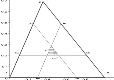
Figure 5: The triangle $\mathscr{T}^{r=\sqrt{2}}$.

The functional forms of the superset region, $\mathscr{R}_{S}\left(N_{PE}^{r},M\right)$, and $T(M_{1},M_{2},M_{3})$ in $T_{b}$ are provided in Ceyhan, (2009).

$N_{PE}^{r}(\cdot,M)$ is geometry invariant if $M$-vertex regions are constructed with $M\in T\left(\mathcal{Y}_{3}\right)^{o}$ by using the extensions of the line segments joining $\mathsf{y}$ to $M$ for all $\mathsf{y}\in\mathcal{Y}_{3}$. But when the vertex regions are constructed by orthogonal projections, $N_{PE}^{r}(\cdot,M)$ is not geometry invariant (Ceyhan, (2009)), hence such vertex regions are not considered here.

6.1.1 Extension of $N_{PE}^{r}$ to Higher Dimensions

The extension to $\mathbb{R}^{d}$ for $d>2$ is straightforward. The extension with $M=M_{C}$ is given her, but the extension for general $M$ is similar. Let $\mathcal{Y}_{d+1}=\{\mathsf{y}_{1},\mathsf{y}_{2},\ldots,\mathsf{y}_{d+1}\}$ be $d+1$ points that do not lie on the same $d-1$-dimensional hyperplane. Denote the simplex formed by these $d+1$ points as $\mathfrak{S}(\mathcal{Y}_{d+1})$. A simplex is the simplest polytope in $\mathbb{R}^{d}$ having $d+1$ vertices, $d\,(d+1)/2$ edges and $d+1$ faces of dimension $(d-1)$. For $r\in[1,\infty]$, define the proximity map as follows. Given a point $x$ in $\mathfrak{S}(\mathcal{Y}_{d+1})$, let $v:=\operatorname{argmin}_{\mathsf{y}\in\mathcal{Y}_{d+1}}\mbox{V}(Q_{\mathsf{y}}(x))$ where $Q_{\mathsf{y}}(x)$ is the polytope with vertices being the $d\,(d+1)/2$ midpoints of the edges, the vertex $v$ and $x$ and $\mbox{V}(\cdot)$ is the $d$-dimensional volume functional. That is, the vertex region for vertex $v$ is the polytope with vertices given by $v$ and the midpoints of the edges. Let $v(x)$ be the vertex in whose region $x$ falls. If $x$ falls on the boundary of two vertex regions, $v(x)$ is assigned arbitrarily. Let $\varphi(x)$ be the face opposite to vertex $v(x)$, and $\Upsilon(v(x),x)$ be the hyperplane parallel to $\varphi(x)$ which contains $x$. Let $d(v(x),\Upsilon(v(x),x))$ be the (perpendicular) Euclidean distance from $v(x)$ to $\Upsilon(v(x),x)$. For $r\in[1,\infty)$, let $\Upsilon_{r}(v(x),x)$ be the hyperplane parallel to $\varphi(x)$ such that

$$d(v(x),\Upsilon_{r}(v(x),x))=r\,d(v(x),\Upsilon(v(x),x))\text{ and }d(\Upsilon(v(x),x),\Upsilon_{r}(v(x),x))<d(v(x),\Upsilon_{r}(v(x),x)).$$

Let $\mathfrak{S}_{r}(x)$ be the polytope similar to and with the same orientation as $\mathfrak{S}$ having $v(x)$ as a vertex and $\Upsilon_{r}(v(x),x)$ as the opposite face. Then the proximity region $N_{PE}^{r}(x,M_{C}):=\mathfrak{S}_{r}(x)\cap\mathfrak{S}(\mathcal{Y}_{d+1})$. Notice that $r\geq 1$ implies $x\in N_{PE}^{r}(x,M_{C})$.

6.1.2 $\Gamma_{1}$-Regions for Proportional-Edge Proximity Maps

For $N_{PE}^{r}(\cdot,M)$, the $\Gamma_{1}$-region is constructed as follows; see also Figure 6. Let $\xi_{i}(r,x)$ be the line parallel to $e_{i}$ such that $\xi_{i}(r,x)\cap T\left(\mathcal{Y}_{3}\right)\not=\emptyset$ and $r\,d(\mathsf{y}_{i},\xi_{i}(r,x))=d(\mathsf{y}_{i},\ell(\mathsf{y}_{i},x))$ for $i\in\{1,2,3\}$. Then

$$\Gamma_{1}\left(x,N_{PE}^{r},M\right)=\bigcup_{i=1}^{3}\bigl{[}\Gamma_{1}\left(x,N_{PE}^{r},M\right)\cap R_{M}(\mathsf{y}_{i})\bigr{]}$$

where

$$\Gamma_{1}\left(x,N_{PE}^{r},M\right)\cap R_{M}(\mathsf{y}_{i})=\{z\in R_{M}(\mathsf{y}_{i}):d(\mathsf{y}_{i},\ell(\mathsf{y}_{i},z))\geq d(\mathsf{y}_{i},\xi_{i}(r,x)\}\text{ for }i\in\{1,2,3\}.$$

Notice that $r\geq 1$ implies $x\in\Gamma_{1}\left(x,N_{PE}^{r},M\right)$. Furthermore, $\lim_{r\rightarrow\infty}\Gamma_{1}\left(x,N_{PE}^{r},M\right)=T\left(\mathcal{Y}_{3}\right)$ for all $x\in T\left(\mathcal{Y}_{3}\right)\setminus\mathcal{Y}_{3}$ and so we define $\Gamma_{1}\left(x,N_{PE}^{r=\infty},M\right)=T\left(\mathcal{Y}_{3}\right)$ for all such $x$. For $x\in\mathcal{Y}_{3}$, $\Gamma_{1}\left(x,N_{PE}^{r},M\right)=\{x\}$ for all $r\in[1,\infty]$.

Figure 6: Construction of the $\Gamma_{1}$-region, $\Gamma_{1}\left(x,N_{PE}^{r=2},M_{C}\right)$ (shaded region).

The functional form of $\Gamma_{1}\left(x=(x_{0},y_{0}),N_{PE}^{r},M\right)$ in the basic triangle $T_{b}$ is given by

$$\Gamma_{1}\left(x=(x_{0},y_{0}),N_{PE}^{r},M\right)=\bigcup_{i=1}^{3}\left[\Gamma_{1}\left(x=(x_{0},y_{0}),N_{PE}^{r},M\right)\cap R_{M}(y_{i})\right]$$

where

$$\Gamma_{1}\left(x=(x_{0},y_{0}),N_{PE}^{r},M\right)\cap R_{M}(\mathsf{y}_{1}) =\left\{(x,y)\in R_{M}(\mathsf{y}_{1}):y\geq\frac{y_{0}}{r}-\frac{c_{2}\,(r\,x-x_{0})}{(1-c_{1})\,r}\right\},$$

$$\Gamma_{1}\left(x=(x_{0},y_{0}),N_{PE}^{r},M\right)\cap R_{M}(\mathsf{y}_{2}) =\left\{(x,y)\in R_{M}(\mathsf{y}_{1}):y\geq\frac{y_{0}}{r}-\frac{c_{2}\,(r\,(x-1)+1-x_{0}}{c_{1}\,r}\right\},$$

$$\Gamma_{1}\left(x=(x_{0},y_{0}),N_{PE}^{r},M\right)\cap R_{M}(\mathsf{y}_{3}) =\left\{(x,y)\in R_{M}(\mathsf{y}_{1}):y\leq\frac{y_{0}-c_{2}\,(1-r)}{r}\right\}.$$

Notice that $\Gamma_{1}\left(x,N_{PE}^{r},M_{C}\right)$ is a convex hexagon for all $r\geq 2$ and $x\in T\left(\mathcal{Y}_{3}\right)\setminus\mathcal{Y}_{3}$, (since for such an $x$, $\Gamma_{1}\left(x,N_{PE}^{r},M_{C}\right)$ is bounded by $\xi_{i}(r,x)$ and $e_{i}$ for all $i\in\{1,2,3\}$, see also Figure 6) else it is either a convex hexagon or a non-convex polygon depending on the location of $x$ and the value of $r$.

Furthermore, in $\mathbb{R}^{d}$ with $d>2$ let $\zeta_{i}(x)$ be the hyperplane such that $\zeta_{i}(x)\cap\mathfrak{S}\left(\mathcal{Y}_{m}\right)\not=\emptyset$ and $r\,d(\mathsf{y}_{i},\zeta_{i}(x))=d(\mathsf{y}_{i},\eta(\mathsf{y}_{i},x))$ for $i=1,2,\ldots,(d+1)$. Then $\Gamma_{1}\left(x,N_{PE}^{r}\right)\cap R_{CM}(\mathsf{y}_{i})=\{z\in R_{CM}(\mathsf{y}_{i}):d(\mathsf{y}_{i},\eta(\mathsf{y}_{i},z))\geq d(\mathsf{y}_{i},\zeta_{i}(x)\}$, for $i=1,2,3$. Hence $\Gamma_{1}\left(x,N_{PE}^{r}\right)=\bigcup_{i=1}^{d+1}(\Gamma_{1}\left(x,N_{PE}^{r}\right)\cap R_{CM}(\mathsf{y}_{i}))$. Notice that $r\geq 1$ implies $x\in N_{PE}^{r}(x)$ and $x\in\Gamma_{1}\left(x,N_{PE}^{r}\right)$.

So far, we have described the $\Gamma_{1}$-region for a point in $x\in T\left(\mathcal{Y}_{3}\right)$. For a set $\mathcal{X}_{n}$ of size $n$ in $T\left(\mathcal{Y}_{3}\right)$, the region $\Gamma_{1}\left(\mathcal{X}_{n},N_{PE}^{r},M\right)$ can be exactly described by the edge extrema.

Definition 6.1.

The (closest) edge extrema of a set $B$ in $T\left(\mathcal{Y}_{3}\right)$ are the points closest to the edges of $T\left(\mathcal{Y}_{3}\right)$, denoted $x_{e_{i}}$ for $i\in\{1,2,3\}$; that is, $x_{e_{i}}\in\operatorname{arginf}_{x\in B}d(x,e_{i})$.

Note that if $B=\mathcal{X}_{n}$ is a random sample of size $n$ from $F$ then the edge extrema, denoted $X_{e_{i}}(n)$, are random variables.

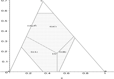
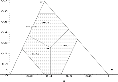
Figure 7: $\Gamma_{1}\left(x,N_{PE}^{2},M_{CC}\right)$ with $x\in R_{CC}(\mathsf{y}_{3})$ (left), $x\in R^{\perp}_{IC}(\mathsf{y}_{3})$ (right).

Proposition 6.2.

Let $B$ be any set of $n$ distinct points in $T\left(\mathcal{Y}_{3}\right)$ and $x_{e_{i}}\in\operatorname{arginf}_{x\in B}d(x,e_{i})$. For proportional-edge proximity maps with $M$-vertex regions, $\Gamma_{1}\left(B,N_{PE}^{r},M\right)=\bigcap_{i=1}^{3}\,\Gamma_{1}\left(x_{e_{i}},N_{PE}^{r},M\right)$.

Proof: Given $B=\{x_{1},x_{2},\ldots,x_{n}\}$ in $T\left(\mathcal{Y}_{3}\right)$. Note that

$$\Gamma_{1}\left(B,N_{PE}^{r},M\right)\cap R_{M}(\mathsf{y}_{i})=\left[\bigcap_{i=1}^{n}\,\Gamma_{1}\left(x_{i},N_{PE}^{r},M\right)\right]\cap R_{M}(\mathsf{y}_{i}),$$

and if $d(\mathsf{y}_{i},\ell(\mathsf{y}_{i},x))\leq d(\mathsf{y}_{i},\ell(\mathsf{y}_{i},x^{\prime}))$ then $N_{PE}^{r}(x,M)\subseteq N_{PE}^{r}(x^{\prime},M)$ for all $x,x^{\prime}\in R_{M}(y_{i})$. Further, by definition $x_{e_{i}}\in\operatorname{argmax}_{x\in B}d(\mathsf{y}_{i},\xi_{i}(r,x))$, so

$$\Gamma_{1}\left(B,N_{PE}^{r},M\right)\cap R_{M}(\mathsf{y}_{i})=\Gamma_{1}\left(x_{e_{i}},N_{PE}^{r},M\right)\cap R_{M}(\mathsf{y}_{i})\text{ for }i\in\{1,2,3\}.$$

Furthermore, $\Gamma_{1}\left(B,N_{PE}^{r},M\right)=\bigcup_{i=1}^{3}\bigl{[}\Gamma_{1}\left(x_{e_{i}},N_{PE}^{r},M\right)\cap R_{M}(\mathsf{y}_{i})\bigr{]}$, and

$$\Gamma_{1}\left(x_{e_{i}},N_{PE}^{r},M\right)\cap R_{M}(\mathsf{y}_{i})=\left[\bigcap_{j=1}^{3}\Gamma_{1}\left(x_{e_{j}},N_{PE}^{r},M\right)\right]\cap R_{M}(\mathsf{y}_{i})\text{ for }i\in\{1,2,3\}.$$

Combining these two results, we obtain $\Gamma_{1}\left(B,N_{PE}^{r},M\right)=\bigcap_{j=1}^{3}\,\Gamma_{1}\left(x_{e_{j}},N_{PE}^{r},M\right)$. $\blacksquare$

From the above proposition, we see that the $\Gamma_{1}$-region for $B$ as in the proposition can also be written as the union of three regions of the form

$$\Gamma_{1}\left(B,N_{PE}^{r},M\right)\cap R_{M}(\mathsf{y}_{i})=\{z\in R_{M}(\mathsf{y}_{i}):\;d(\mathsf{y}_{i},\ell(\mathsf{y}_{i},z))\geq d(\mathsf{y}_{i},\xi_{i}(r,x_{e_{i}}))\}\text{ for }i\in\{1,2,3\}.$$

Corollary 6.3.

Let $\mathcal{X}_{n}$ be a random sample from a continuous distribution $F$ on $T\left(\mathcal{Y}_{3}\right)$. For proportional-edge proximity maps with $M$-vertex regions, $\eta_{n}\left(N_{PE}^{r}\right)\leq 3$ with equality holding with positive probability for $n\geq 3$.

Proof: From Proposition 6.2, $\eta_{n}\left(N_{PE}^{r}\right)\leq 3$. Furthermore, $X_{e}(n)$ is unique for each edge $e$ a.s. since $F$ is continuous, and there are three distinct edge extrema with positive probability. Hence $P(\eta_{n}\left(N_{PE}^{r}\right)=3)>0$ for $n\geq 3$. $\blacksquare$

Then $\Gamma_{1}\left(\mathcal{X}_{n},N_{PE}^{r},M\right)=\bigcap_{i=1}^{3}\Gamma_{1}\left(X_{e_{i}},N_{PE}^{r}\right)$, where $e_{i}$ is the edge opposite vertex $\mathsf{y}_{i}$, for $i=1,2,3$. So $\Gamma_{1}\left(\mathcal{X}_{n},N_{PE}^{r},M\right)\cap R_{M}(\mathsf{y}_{i})=\{z\in R_{M}(\mathsf{y}_{i}):\;d(\mathsf{y}_{i},\ell(\mathsf{y}_{i},z))\geq d(\mathsf{y}_{i},\xi_{i}(r,x_{e_{i}}))\}$, for $i=1,2,3$.

Note that $P(\eta_{n}\left(N_{PE}^{r}\right)=3)\rightarrow 1$ as $n\rightarrow\infty$ for $\mathcal{X}_{n}$ a random sample from $\mathcal{U}(T\left(\mathcal{Y}_{3}\right))$, since edge extrema are distinct with probability 1 as $n\rightarrow\infty$ as shown in the following theorem.

Theorem 6.4.

Let $\mathcal{X}_{n}$ be a random sample from $\mathcal{U}(T\left(\mathcal{Y}_{3}\right))$ and let $E_{c,3}(n)$ be the event that (closest) edge extrema are distinct. Then $P(E_{c,3}(n))\rightarrow 1$ as $n\rightarrow\infty$.

Proof: Using the uniformity preserving transformation $\phi_{e}$ without loss of generality, one can assume $\mathcal{X}_{n}$ is a random sample from $\mathcal{U}(T_{e})$. Observe also that the edge extrema in $T_{b}$ are mapped into the edge extrema in $T_{e}$. Note that the probability of edge extrema all being equal to each other is $P(X_{e_{1}}(n)=X_{e_{2}}(n)=X_{e_{3}}(n))=\mathbf{I}(n=1)$. Let $E_{c,2}(n)$ be the event that there are only two distinct (closest) edge extrema. Then for $n>1$,

$$P(E_{c,2}(n))=P(X_{e_{1}}(n)=X_{e_{2}}(n))+P(X_{e_{1}}(n)=X_{e_{3}}(n))+P(X_{e_{2}}(n)=X_{e_{3}}(n))$$

since the intersection of events $X_{e_{1}}(n)=X_{e_{2}}(n))$, $X_{e_{1}}(n)=X_{e_{3}}(n)$, and $X_{e_{2}}(n)=X_{e_{3}}(n)$ is equivalent to the event $X_{e_{1}}(n)=X_{e_{2}}(n)=X_{e_{3}}(n)$. Notice also that $P(E_{c,2}(n=2))=1$. So, for $n>2$, there are two or three distinct edge extrema with probability 1; i.e., $P(E_{c,3}(n))+P(E_{c,2}(n))=1$ for $n>2$.

We will show that $P(E_{c,2}(n))\rightarrow 0$ as $n\rightarrow\infty$, which will imply the desired result.

First consider $P(X_{e_{1}}(n)=X_{e_{2}}(n))$. The event $X_{e_{1}}(n)=X_{e_{2}}(n)=X_{e}=(X,Y)$ is equivalent to the event that $\mathcal{X}_{n}\subset\{U\in T_{e}:\;d(\mathsf{y}_{1},\ell(\mathsf{y}_{1},U))\leq d(\mathsf{y}_{1},\ell(\mathsf{y}_{1},X_{e})),\;d(\mathsf{y}_{2},\ell(\mathsf{y}_{2},U))\leq d(\mathsf{y}_{2},\ell(\mathsf{y}_{2},X_{e}))\}$. For example, if given $X_{e_{1}}(n)=X_{e_{2}}(n)=(x,y)$ the remaining $n-1$ points will lie in the shaded region in Figure 8 (left). For other pairs of edge extrema, see Figures 8 (right) and 9.

The pdf of such $X_{e}=(X,Y)$ is $f(x,y)=n\,\left(4/\sqrt{3}\right)\,\left(y^{2}/\sqrt{3}\right)^{n-1}$. Let $\varepsilon>0$, by Markov’s inequality, $P\left(\sqrt{3}/2-Y>\varepsilon\right)\leq\mathbf{E}\,\left[\sqrt{3}/2-Y\right]/\varepsilon$. But,

$$\mathbf{E}\,\left[\sqrt{3}/2-Y\right] = \int_{0}^{1/2}\int_{0}^{\sqrt{3}\,x}\left(\sqrt{3}/2-y\right)\,n\,\left(y^{2}/\sqrt{3}\right)^{n-1}\,\left(4/\sqrt{3}\right)dy\,dx$$

$$+\int_{1/2}^{1}\int_{0}^{\sqrt{3}\,(1-x)}\left(\sqrt{3}/2-y\right)\,n\,\left(y^{2}/\sqrt{3}\right)^{n-1}\,\left(4/\sqrt{3}\right)dy\,dx$$

$$= 4\,\left(\sqrt{3}/4\right)^{n}\frac{1}{n\,(4\,n^{2}-1)},$$

which converges to 0 as $n\rightarrow\infty$. So if $X_{e_{1}}(n)=X_{e_{2}}(n)$ were the case, then geometric locus of this point goes to $\mathsf{y}_{3}$. That is, for each $\varepsilon>0$, $P\left(\sqrt{3}/2-Y>\varepsilon\right)\rightarrow 0$ as $n\rightarrow\infty$. Hence $P(X_{e_{1}}(n)=X_{e_{2}}(n)\not=\mathsf{y}_{3})\rightarrow 0$ as $n\rightarrow\infty$. Furthermore, $P(X_{e_{1}}(n)=X_{e_{2}}(n)=\mathsf{y}_{3})\leq P(X_{e_{2}}(n)\in e_{2})=0$ for all $n\geq 1$. So $P(X_{e_{1}}(n)=X_{e_{2}}(n))\rightarrow 0$ as $n\rightarrow\infty$.

Likewise, by symmetry, it follows that $\lim_{n\rightarrow\infty}P(X_{e_{1}}(n)=X_{e_{3}}(n))=\lim_{n\rightarrow\infty}P(X_{e_{2}}(n)=X_{e_{3}}(n))=0$. Hence $P(E_{c,2}(n))\rightarrow 0$ as $n\rightarrow\infty$. Thus $P(E_{c,3}(n))\rightarrow 1$ as $n\rightarrow\infty$. $\blacksquare$

The above theorem implies that the asymptotic distribution of $\eta_{n}\left(N_{PE}^{r}\right)$ is degenerate with $P(\eta_{n}\left(N_{PE}^{r}\right)=3)\rightarrow 1$ as $n\rightarrow\infty$. But for finite $n$, $\eta_{n}\left(N_{PE}^{r}\right)$ for $X_{i}\stackrel{{\scriptstyle iid}}{{\sim}}\mathcal{U}(T\left(\mathcal{Y}_{3}\right))$ has the following non-degenerate distribution.

$$\eta_{n}\left(N_{PE}^{r}\right)~{}=~{}\left\{\begin{array}[]{ll}2{}{}{}&\mbox{wp $\pi_{2}(n)$}\\[4.30554pt] 3&\mbox{wp $\pi_{3}(n)=1-\pi_{2}(n)$,}\end{array}\right.$$

where $\pi_{2}(n)\in(0,1)$ is the probability of edge extrema for any two distinct edges being concurrent.

Figure 8: The figure for $X_{e_{1}}(n)=X_{e_{2}}(n)=(x,y)$ (left) and $X_{e_{2}}(n)=X_{e_{3}}(n)=(x,y)$ (right).

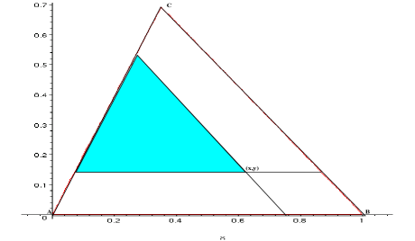
Figure 9: The figure for $X_{e_{1}}(n)=X_{e_{3}}(n)=(x,y)$.

Remark 6.5.

If $\mathcal{X}_{n}$ is a random sample from $F$ such that $\mathcal{S}(F)\cap\{x\in T\left(\mathcal{Y}_{3}\right):\;d(x,e_{i})\leq\varepsilon_{1}\}$ has positive measure and $\mathcal{S}(F)\cap B(\mathsf{y}_{i},\varepsilon_{2})=\emptyset$ for some $\varepsilon_{1},\varepsilon_{2}>0$, then $P(E_{c,3}(n))\rightarrow 1$ as $n\rightarrow\infty$ follows trivially. However, the case that $F$ has positive density around the vertices $\mathcal{Y}_{3}$ requires more work to prove as shown below. $\square$

Theorem 6.6.

Let $\mathcal{X}_{n}$ be a random sample from $F$ such that $B(\mathsf{y}_{i},\varepsilon)\subseteq\mathcal{S}(F)$ for some $\varepsilon>0$ and for each $i=1,2,3$, then $P(E_{c,3}(n))\rightarrow 1$ as $n\rightarrow\infty$.

Proof: Using the transformation $\phi_{e}:\,(x,y)\rightarrow(u,v)$, above, we can without loss of generality assume $\mathcal{X}_{n}$ is a random sample from $F$ with support $\mathcal{S}(F)\subseteq T_{e}$. After $\phi_{e}$ is applied, suppose $F$ becomes $F_{e}$, then $\phi_{e}(\mathcal{X}_{n})$ becomes a random sample from $F_{e}$ such that $B(\phi_{e}(\mathsf{y}_{i}),\varepsilon_{e})\subseteq\mathcal{S}(F_{e})$ for some $\varepsilon_{e}>0$ and for each $i=1,2,3$. First consider $P(X_{e_{1}}=X_{e_{3}})$. Given $X_{e_{1}}=X_{e_{3}}=(x,y)$ the remaining $n-1$ points will lie in the shaded region in Figure 8 (right). $X_{e_{1}}=X_{e_{3}}=(X,Y)$ is equivalent to the event that

$$\mathcal{X}_{n}\subset S_{R}(X,Y):=\{(U,W)\in T_{e}:\;\ell(\mathsf{y}_{1},(U,W))\leq\ell(\mathsf{y}_{1},(X,Y)),\;\ell(\mathsf{y}_{3},(U,W))\leq\ell(\mathsf{y}_{3},(X,Y))\}.$$

The pdf of such $(X,Y)$ is $f(x,y)=n\,G(x,y)^{n-1}\,f(x,y)$ where $G(u,v):=P_{F}(X\in S_{R}(u,v))$. Note that $P(X_{e_{2}}=X_{e_{3}}=\mathsf{y}_{1})=0$ for all $n$, and $X_{e_{2}}=X_{e_{3}}\not=\mathsf{y}_{1}$ is equivalent to $d((X,Y),\mathsf{y}_{1})>0$. Let $\varepsilon>0$, by Markov’s inequality, $P(d((X,Y),\mathsf{y}_{1})>\varepsilon)\leq\mathbf{E}\,\left[d((X,Y),\mathsf{y}_{1})\right]/\varepsilon=\mathbf{E}\,\left[\sqrt{X^{2}+Y^{2}}\right]/\varepsilon$. Switching to the polar coordinates as $X=R\,\cos\theta$ and $Y=R\,\sin\theta$, we get $\sqrt{X^{2}+Y^{2}}=R$. But, $\displaystyle\mathbf{E}\,[R]=\int_{0}^{\varepsilon}\int_{0}^{\pi/3}n\,r\,G(r,\theta)^{n-1}\,f(r,\theta)r\,dr\,d\theta$. Integrand is critical at $r=0$, since for $r>0$ it converges to zero as $n\rightarrow\infty$. So we use the Taylor series expansion around $r=0$ as

$$f(r,\theta) =f(0,\theta)+\frac{\partial{f(0,\theta)}}{\partial r}r+O\left(r^{2}\right),$$

$$G(r,\theta) =G(0,\theta)+\frac{\partial{G(0,\theta)}}{\partial r}r+O\left(r^{2}\right)=1+\frac{\partial{G(0,\theta)}}{\partial r}r+O\left(r^{2}\right).$$

Note that $\displaystyle\frac{\partial{G(0,\theta)}}{\partial r}<0$, since area of $S_{R}(u,v)$ decreases as $r$ increases for fixed $\theta$. So let $r=w/n$, then

$$\mathbf{E}\,[R] \sim \int_{0}^{n\,\varepsilon}\int_{0}^{\pi/3}n\,\frac{w}{n}\,\left(1+\frac{\partial{G(0,\theta)}}{\partial r}\frac{w}{n}+O\left(n^{-2}\right)\right)^{n-1}\,\left(f(0,\theta)+\frac{\partial{f(0,\theta)}}{\partial r}\frac{w}{n}+O\left(n^{-2}\right)\right)\frac{w}{n^{2}}\,dw\,d\theta$$

$$= \frac{1}{n^{2}}\int_{0}^{\infty}\int_{0}^{\pi/3}w^{2}\,\exp\left(\frac{\partial{G(0,\theta)}}{\partial r}w\right)\,f(0,\theta)w\,dw\,d\theta=O\left(n^{-2}\right).$$

Hence $P(X_{e_{2}}=X_{e_{3}}\not=\mathsf{y}_{1})\rightarrow 0$ as $n\rightarrow\infty$. Then $P(X_{e_{2}}=X_{e_{3}})\rightarrow 0$ as $n\rightarrow\infty$.

Likewise, it follows that $\lim_{n\rightarrow\infty}P(X_{e_{1}}=X_{e_{2}})=\lim_{n\rightarrow\infty}P(X_{e_{1}}=X_{e_{3}})=0$. Hence $P(E_{c,2}(n))\rightarrow 0$ as $n\rightarrow\infty$. Thus $P(E_{c,3}(n))\rightarrow 1$ as $n\rightarrow\infty$. $\blacksquare$

Notice that Theorem 6.4 follows as a corollary from Theorem 6.6. For $r\geq 3/2$ and $M\in\mathbb{R}^{2}\setminus\mathcal{Y}_{3}$, $\Gamma_{1}\left(\mathcal{X}_{n},N_{PE}^{r},M\right)\not=\emptyset$ a.s., since $\mathscr{R}_{S}\left(N_{PE}^{r},M\right)\not=\emptyset$ and $\mathscr{R}_{S}\left(N_{PE}^{r},M\right)\subseteq\Gamma_{1}\left(\mathcal{X}_{n},N_{PE}^{r},M\right)$.

Now, for $n>1$, let $X_{e_{i}}(n)=x_{e_{i}}=(u_{i},w_{i})$ be given for $i\in\{1,2,3\},$ be the edge extrema in a given realization of $\mathcal{X}_{n}$. Then the functional form of $\Gamma_{1}$-region in $T_{b}$ is given by

$$\Gamma_{1}\left(\mathcal{X}_{n},N_{PE}^{r},M\right)=\bigcup_{i=1}^{3}\bigl{[}\Gamma_{1}\left(\mathcal{X}_{n},N_{PE}^{r},M\right)\cap R_{M}(\mathsf{y}_{i})\bigr{]}$$

where

$$\Gamma_{1}\left(\mathcal{X}_{n},N_{PE}^{r},M\right)\cap R_{M}(\mathsf{y}_{1}) =\left\{(x,y)\in R_{M}(\mathsf{y}_{1}):y\geq\frac{w_{1}}{r}-\frac{c_{2}\,(r\,x-u_{1})}{(1-c_{1})\,r}\right\},$$

$$\Gamma_{1}\left(\mathcal{X}_{n},N_{PE}^{r},M\right)\cap R_{M}(\mathsf{y}_{2}) =\left\{(x,y)\in R_{M}(\mathsf{y}_{1}):y\geq\frac{w_{2}}{r}-\frac{c_{2}\,(r\,(x-1)+1-u_{2}}{c_{1}\,r}\right\},$$

$$\Gamma_{1}\left(\mathcal{X}_{n},N_{PE}^{r},M\right)\cap R_{M}(\mathsf{y}_{3}) =\left\{(x,y)\in R_{M}(\mathsf{y}_{1}):y\leq\frac{w_{3}-c_{2}\,(1-r)}{r}\right\}.$$

See Figure 10 for $\Gamma_{1}\left(\mathcal{X}_{n},N_{PE}^{2},M\right)$ with $n\geq 3$ where $M$-vertex regions for $M=M_{CC}$ and $M=M_{I}$ with orthogonal projections are used. Note that only the edge extrema are shown in Figure 10 (right).

Figure 10: $\Gamma_{1}\left(\mathcal{X}_{n},N_{PE}^{2},M\right)$ for $M=M_{CC}$ (left) and $M=M_{I}$ (right) with three distinct edge extrema.

Note that, for $\mathcal{X}_{n}$ a random sample from $\mathcal{U}(T\left(\mathcal{Y}_{3}\right))$, $P(\eta_{n}\left(N_{PE}^{r}\right)=3)\rightarrow 1$ as $n\rightarrow\infty$, since the edge extrema are distinct with probability 1 as $n\rightarrow\infty$. However, for $r<3/2$, the region $\Gamma_{1}\left(x,N_{PE}^{r},M\right)\cap R_{M}(\mathsf{y}_{i})$ might be empty for some $i\in\{1,2,3\}$. Furthermore, if $M\in(\mathscr{T}^{r})^{o}$ (see Equation (3) for $\mathscr{T}^{r}$) with $r<3/2$, then $\Gamma_{1}\left(\mathcal{X}_{n},N_{PE}^{r},M\right)$ will be empty with probability 1 as $n\rightarrow\infty$. In such a case, there is no $\Gamma_{1}$-region to construct. But the definition of the $\eta$-value still works in the sense that $\Gamma_{1}\left(X_{n},N_{PE}^{r},M\right)=\emptyset=\bigcap_{x\in S_{M}}\Gamma_{1}\left(x,N_{PE}^{r},M\right)$ (see Definition 4.4 for $S_{M}$) and $\Gamma_{1}\left(x,N_{PE}^{r},M\right)\not=\emptyset$ for all $x\in\mathcal{X}_{n}$ since $x\in\Gamma_{1}\left(x,N_{PE}^{r},M\right)$. To determine whether the $\Gamma_{1}$-region is empty or not, it suffices to check the intersection of the $\Gamma_{1}$-regions of the edge extrema. If $M\notin(\mathscr{T}^{r})^{o}$, the $\Gamma_{1}$-region is guaranteed to be nonempty.

Note that $\eta_{n}\left(N_{PE}^{r_{1}}\right)\stackrel{{\scriptstyle d}}{{=}}\eta_{n}\left(N_{PE}^{r_{2}}\right)$ for all $(r_{1},\,r_{2})\in[1,\infty)^{2}$, where $\stackrel{{\scriptstyle d}}{{=}}$ stands for “equality in distribution”.

See Figure 12 for $\Gamma_{1}\left(\mathcal{X}_{n},N_{PE}^{\sqrt{2}},M\right)$ where $M$-vertex regions for $M=M_{CC}$ and $M=M_{I}$ with orthogonal projections are used.

Figure 11: $\Gamma_{1}\left(x,N_{PE}^{\sqrt{2}},M\right)$ with $x\in R_{CC}(\mathsf{y}_{3})$ (left), $x\in R^{\perp}_{IC}(\mathsf{y}_{3})$.

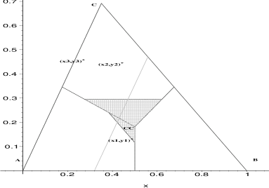
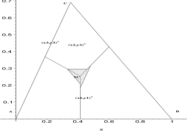
Figure 12: $\Gamma_{1}\left(\mathcal{X}_{n},N_{PE}^{\sqrt{2}},M\right)$ for $M=M_{CC}$ (left) and $M=M_{I}$ (right) with three distinct edge extrema.

Remark 6.7.

• For $r_{1}<r_{2}$, $\Gamma_{1}\left(x,N_{PE}^{r_{1}},M\right)\subseteq\Gamma_{1}\left(x,N_{PE}^{r_{2}},M\right)$ for all $x\in T\left(\mathcal{Y}_{3}\right)$ with equality holding only when $x\in\mathcal{Y}_{3}$.

• For $r_{1}<r_{2}$, $\Gamma_{1}\left(\mathcal{X}_{n},N_{PE}^{r_{1}},M\right)\subseteq\Gamma_{1}\left(\mathcal{X}_{n},N_{PE}^{r_{2}},M\right)$ with equality holding only when $\mathcal{X}_{n}\subseteq\mathcal{Y}_{3}$ or $\Gamma_{1}\left(\mathcal{X}_{n},N_{PE}^{r},M\right)=\emptyset$ for $r=r_{1},r_{2}$.

• Suppose $X,Y$ are iid from a continuous distribution $F$ whose support is $\mathcal{S}(F)\subseteq T\left(\mathcal{Y}_{3}\right)$. Then for $r_{1}<r_{2}$, $A\left(\Gamma_{1}\left(X,N_{PE}^{r_{1}},M\right)\right)\leq^{ST}A\left(\Gamma_{1}\left(Y,N_{PE}^{r_{2}},M\right)\right)$.

• Suppose $\mathcal{X}_{n}$ and $\mathcal{X}^{\prime}_{n}$ are two random samples from a continuous distribution $F$ whose support is $\mathcal{S}(F)\subseteq T\left(\mathcal{Y}_{3}\right)$. Then for $r_{1}<r_{2}$, $A(\Gamma_{1}\left(\mathcal{X}_{n},N_{PE}^{r_{1}},M\right))\leq^{ST}A(\Gamma_{1}\left(\mathcal{X}^{\prime}_{n},N_{PE}^{r_{2}},M\right))$. $\square$

Remark 6.8.

In $\mathbb{R}^{d}$ with $d>2$, recall $\mathfrak{S}\left(\mathcal{Y}_{m}\right)$, the simplex based on $d+1$ points that do not lie on the same hyperplane. Furthermore, let $\varrho_{i}(r,x)$ be the hyperplane such that $\varrho_{i}(x)\cap\mathfrak{S}\left(\mathcal{Y}_{m}\right)\not=\emptyset$ and $r\,d(\mathsf{y}_{i},\varrho_{i}(r,x))=d(\mathsf{y}_{i},\Upsilon(\mathsf{y}_{i},x))$ for $i\in\{1,2,\ldots,d+1$. Then

$$\Gamma_{1}\left(x,N_{PE}^{r},M_{C}\right)\cap R_{CM}(\mathsf{y}_{i})=\{z\in R_{CM}(\mathsf{y}_{i}):d(\mathsf{y}_{i},\Upsilon(\mathsf{y}_{i},z))\geq d(\mathsf{y}_{i},\varrho_{i}(r,x)\}\text{ for }i\in\{1,2,3\}.$$

Hence $\Gamma_{1}\left(x,N_{PE}^{r},M_{C}\right)=\bigcup_{i=1}^{d+1}(\Gamma_{1}\left(x,N_{PE}^{r},M_{C}\right)\cap R_{CM}(\mathsf{y}_{i}))$. Furthermore, it is easy to see that $\Gamma_{1}\left(\mathcal{X}_{n},N_{PE}^{r},M_{C}\right)=\bigcap_{i=1}^{d+1}\Gamma_{1}\left(X_{\varphi_{i}}(n),N_{PE}^{r},M_{C}\right)$, where $X_{\varphi_{i}}(n)$ is one of the closest points in $\mathcal{X}_{n}$ to face $\varphi_{i}$. $\square$

6.2 Central Similarity Proximity Maps

The other type of triangular proximity map we introduce is the central similarity proximity map. Furthermore, the relative density of the corresponding PCD will have mathematical tractability. Alas, the distribution of the domination number of the associated PCD is still an open problem.

For $\tau\in[0,1]$, define $N_{CS}^{\tau}(\cdot,M):=N(\cdot,M;\tau,\mathcal{Y}_{3})$ to be the central similarity proximity map with $M$-edge regions as follows; see also Figure 13 with $M=M_{C}$. For $x\in T\left(\mathcal{Y}_{3}\right)\setminus\mathcal{Y}_{3}$, let $e(x)$ be the edge in whose region $x$ falls; i.e., $x\in R_{M}(e(x))$. If $x$ falls on the boundary of two edge regions, we assign $e(x)$ arbitrarily. For ${\tau}\in(0,1]$, the parametrized central similarity proximity region $N_{CS}^{\tau}(x,M)$ is defined to be the triangle $T_{\tau}(x)$ with the following properties:

• $T_{\tau}(x)$ has edges $e^{\tau}_{i}(x)$ parallel to $e_{i}$ for each $i\in\{1,2,3\}$, and for $x\in R_{M}(e(x))$, $d(x,e^{\tau}(x))=\tau\,d(x,e(x))$ and $d(e^{\tau}(x),e(x))\leq d(x,e(x))$ where $d(x,e(x))$ is the Euclidean (perpendicular) distance from $x$ to $e(x)$;

• $T_{\tau}(x)$ has the same orientation as and is similar to $T\left(\mathcal{Y}_{3}\right)$;

• $x$ is the same type of center of $T_{\tau}(x)$ as $M$ is of $T\left(\mathcal{Y}_{3}\right)$.

Note that (i) implies the parametrization of the proximity region, (ii) explains “similarity”, and (iii) explains “central” in the name, central similarity proximity map. For $\tau=0$, we define $N_{CS}^{\tau=0}(x,M)=\{x\}$ for all $x\in T\left(\mathcal{Y}_{3}\right)$. For $x\in\partial(T\left(\mathcal{Y}_{3}\right))$, we define $N_{CS}^{\tau}(x,M)=\{x\}$ for all $\tau\in[0,1]$.

Notice that by definition $x\in N_{CS}^{\tau}(x,M)$ for all $x\in T\left(\mathcal{Y}_{3}\right)$. Furthermore, $\tau\leq 1$ implies that $N_{CS}^{\tau}(x,M)\subseteq T\left(\mathcal{Y}_{3}\right)$ for all $x\in T\left(\mathcal{Y}_{3}\right)$ and $M\in T\left(\mathcal{Y}_{3}\right)^{o}$. For all $x\in T\left(\mathcal{Y}_{3}\right)^{o}\cap R_{M}(e(x))$, the edges $e^{\tau}(x)$ and $e(x)$ are coincident iff $\tau=1$.

Notice that $X_{i}\stackrel{{\scriptstyle iid}}{{\sim}}F$, with the additional assumption that the non-degenerate two-dimensional probability density function $f$ exists with support $\mathcal{S}(F)\subseteq T\left(\mathcal{Y}_{3}\right)$, implies that the special case in the construction of $N_{CS}^{\tau}(\cdot)$ — $X$ falls on the boundary of two edge regions — occurs with probability zero. Note that for such an $F$, $N_{CS}^{\tau}(X,M)$ is a triangle a.s.

Figure 13: Construction of central similarity proximity region, $N_{CS}^{\tau=1/2}(x,M_{C})$ (shaded region).

Central similarity proximity maps are defined with $M$-edge regions for $M\in T\left(\mathcal{Y}_{3}\right)^{o}$. In general, for central similarity proximity regions with $M$-edge regions, the similarity ratio of $N_{CS}^{\tau}(x,M)$ to $T\left(\mathcal{Y}_{3}\right)$ is $d(x,e^{\tau}(x))/d(M,e(x))$. See Figure 13 for $N_{CS}^{\tau=1/2}(x,M_{C})$ with $e=e_{3}$. The functional form of $N_{CS}^{\tau}(x,M_{C})$ is provided in Ceyhan, (2009).

6.2.1 Extension of $N^{\tau}_{CS}$ to Higher Dimensions

The extension of $N^{\tau}_{CS}$ to $\mathbb{R}^{d}$ for $d>2$ is straightforward. the extension for $M=M_{C}$ is described, the extension for general $M$ is similar. Let $\mathcal{Y}_{d+1}=\{\mathsf{y}_{1},\mathsf{y}_{2},\ldots,\mathsf{y}_{d+1}\}$ be $d+1$ points that do not lie on the same $(d-1)$-dimensional hyperplane. Denote the simplex formed by these $d+1$ points as $\mathfrak{S}(\mathcal{Y}_{d+1})$. For $\tau\in(0,1]$, define the central similarity proximity map as follows. Let $\varphi_{i}$ be the face opposite vertex $\mathsf{y}_{i}$ for $i\in\{1,2,\ldots,(d+1)\}$, and “face regions” $R_{CM}(\varphi_{1}),R_{CM}(\varphi_{2}),\ldots,R_{CM}(\varphi_{d+1})$ partition $\mathfrak{S}(\mathcal{Y}_{d+1})$ into $d+1$ regions, namely the $d+1$ polytopes with vertices being the center of mass together with $d$ vertices chosen from $d+1$ vertices. For $x\in\mathfrak{S}(\mathcal{Y}_{d+1})\setminus\mathcal{Y}_{d+1}$, let $\varphi(x)$ be the face in whose region $x$ falls; $x\in R(\varphi(x))$. If $x$ falls on the boundary of two face regions, $\varphi(x)$ is assigned arbitrarily. For ${\tau}\in(0,1]$, the central similarity proximity region $N_{CS}^{\tau}(x,M_{C})=\mathfrak{S}_{\tau}(x)$ is defined to be the simplex $\mathfrak{S}_{\tau}(x)$ with the following properties:

• $\mathfrak{S}_{\tau}(x)$ has faces $\varphi^{\tau}_{i}(x)$ parallel to $\varphi_{i}(x)$ for $i\in\{1,2,\ldots,(d+1)\}$, and for $x\in R_{CM}(\varphi(x))$, $\tau\,d(x,\varphi(x))=d(\varphi^{\tau}(x),x)$ where $d(x,\varphi(x))$ is the Euclidean (perpendicular) distance from $x$ to $\varphi(x)$;

• $\mathfrak{S}_{\tau}(x)$ has the same orientation as and similar to $\mathfrak{S}(\mathcal{Y}_{d+1})$;

• $x$ is the center of mass of $\mathfrak{S}_{\tau}(x)$, as $M_{C}$ is of $\mathfrak{S}(\mathcal{Y}_{d+1})$. Note that $\tau>1$ implies that $x\in N_{CS}^{\tau}(x)$.

6.2.2 $\Gamma_{1}$-Regions for Central Similarity Proximity Maps

For $N_{CS}^{\tau}$, the $\Gamma_{1}$-region is constructed as follows. Let $e^{\tau}_{i}(x)$ be the edge of $T_{\tau}(x)$ parallel to edge $e_{i}$ for $i\in\{1,2,3\}$. Now, suppose $u\in R_{M}(e_{3})$ and let $\zeta_{i}(\tau,x)$ for $i\in\{1,2,\ldots,7\}$ be the lines such that

$$v\in\zeta_{1}(\tau,u)\cap R_{M}(e_{3}) \Longrightarrow u\in e^{\tau}_{1}(v), v\in\zeta_{5}(\tau,u)\cap R_{M}(e_{2}) \Longrightarrow u\in e^{\tau}_{3}(v),$$

$$v\in\zeta_{2}(\tau,u)\cap R_{M}(e_{3}) \Longrightarrow u\in e^{\tau}_{2}(v), v\in\zeta_{6}(\tau,u)\cap R_{M}(e_{2}) \Longrightarrow u\in e^{\tau}_{2}(v),$$ (4)

$$v\in\zeta_{3}(\tau,u)\cap R_{M}(e_{1}) \Longrightarrow u\in e^{\tau}_{2}(v), v\in\zeta_{7}(\tau,u)\cap R_{M}(e_{3}) \Longrightarrow u\in e^{\tau}_{3}(v).$$

$$v\in\zeta_{4}(\tau,u)\cap R_{M}(e_{1}) \Longrightarrow u\in e^{\tau}_{3}(v),$$

Then $\Gamma_{1}\left(x,N_{CS}^{\tau},M\right)$ is the region bounded by these lines. See also Figure 14. $\Gamma_{1}\left(x,N_{CS}^{\tau},M\right)$ for $x\in R_{M}(e_{i})$ for $i\in\{1,2\}$ can be described similarly.

Notice that $\tau>0$ implies that $x\in\Gamma_{1}\left(x,N_{CS}^{\tau},M\right)$. Furthermore, $\Gamma_{1}\left(x,N_{CS}^{\tau},M\right)=\{x\}$ iff (i) $\tau=0$ or (ii) $x\in\partial(T\left(\mathcal{Y}_{3}\right))$.

The $\Gamma_{1}$-region $\Gamma_{1}\left(x,N_{CS}^{\tau},M\right)$ is a convex $k$-gon with $3\leq k\leq 7$ vertices. In particular, for $\tau=1$, $\Gamma_{1}\left(x,N_{CS}^{\tau=1},M\right)$ is a convex hexagon. See Figure 16 (left).

Figure 14: Examples of the four types of the $\Gamma_{1}$-region, $\Gamma_{1}\left(x,N_{CS}^{\tau=1/2},M_{C}\right)$ with four distinct $x\in R_{CM}(e_{3})$ (shaded regions).

Then the functional form of $\zeta_{i}(x)$ in Equation (6.2.2) that define the boundary of $\Gamma_{1}\left(x=(x_{0},y_{0}),N_{CS}^{\tau}\right)$ with $M$-central proximity regions in the basic triangle $T_{b}$ for $x\in R_{M}(e_{3})$ is

$$\zeta_{1}(x) =\frac{m_{2}\,(c_{2}\,(x-x_{0})+y_{0}\,c_{1})}{m_{2}\,c_{1}\,(1-\tau)+c_{2}\,\tau\,m_{1}},\;\;\zeta_{2}(x)=\frac{m_{2}\,(c_{2}\,(x_{0}-x)+y_{0}\,(1-c_{1}))}{m_{2}\,(1-c_{1})\,(1-\tau)+c_{2}\,\tau\,(1-m_{1})},$$

$$\zeta_{3}(x) =\frac{m_{2}\,c_{2}\,(x-1)+y_{0}\,(m_{2}\,(1-c_{1})-\,c_{2}\,(1-m_{2}))}{c_{1}\,(1-c_{1})\,(1-\tau)},$$

$$\zeta_{4}(x) =\Bigl{[}c_{1}\,(m_{2}\,(1-c_{1})+c_{2}\,(1-m_{1}))\,y_{0}+c_{2}\,(m_{2}\,(1-c_{1})+c_{2}\,(1-m_{1}))\,x_{0}+c_{2}\,(\tau\,(m_{2}\,c_{1}-m_{1}\,c_{2})$$

$$+c_{2}\,(1-m_{1})+m_{2}\,(1-c_{1}))\,x+c_{2}\,\tau\,(m_{1}\,c_{2}-m_{2}\,c_{1})\Bigr{]}\Big{/}\Bigl{[}c_{2}\,(\tau-c_{1}\,(1-\tau))\,m_{1}$$

$$+c_{1}\,(1-c_{1})\,(1-\tau)\,m_{2}+c_{1}\,c_{2}\Bigr{]},$$

$$\zeta_{5}(x) =\frac{\tau\,m_{2}\,c_{2}\,x-y_{0}\,(c_{1}\,m_{2}-c_{2}\,m_{1})}{c_{2}\,m_{1}-c_{1}\,m_{2}\,(1-\tau)},\;\;\zeta_{7}(x)=\frac{y_{0}}{1-\tau}$$

$$\zeta_{6}(x) =\Bigl{[}(1-c_{1})\,c_{1}\,(m_{2}\,(1-c_{1})-c_{2}\,(1-m_{1}))\,y_{0}+c_{1}\,c_{2}\,(m_{2}\,(1-c_{1})-c_{2}\,(1-m_{1}))\,x_{0}+(c_{2}^{2}\,c_{1}\,(1-\tau)\,m_{1}$$

$$+c_{2}\,\tau\,(1-c_{1})+(1-\tau)\,(c_{1}\,c_{2}-c_{1}^{2}\,c_{2})\,m_{2}-c_{2}^{2}\,\tau\,(1-c_{1})-c_{2}^{2}\,c_{1}\,(1-\tau))\,x+c_{2}^{2}\,\tau\,(m_{1}-c_{1})\Bigr{]}\Big{/}\Bigl{[}(1-c_{1})\,$$

$$(c_{2}\,(c_{2}\,(1-\tau)-\tau)\,m_{1}+c_{1}\,(1-c_{1})\,(1-\tau)\,m_{2}+c_{1}\,c_{2}\,(1-2\,\tau))\Bigr{]}$$

Proposition 6.9.

Let $\mathcal{X}_{n}$ be a random sample from $\mathcal{U}(T\left(\mathcal{Y}_{3}\right))$. For central similarity proximity maps with $M$-edge regions (by definition $M\in T\left(\mathcal{Y}_{3}\right)^{o}$) and $\tau>0$, $\eta_{n}\left(N_{CS}^{\tau}\right)\leq 3$ with equality holding with positive probability for $n\geq 3$.

Proof: Let $M\in T\left(\mathcal{Y}_{3}\right)^{o}$ and $\tau>0$. Then given $\mathcal{X}_{n}$, for $i\in\{1,2,3\}$, we have

$$\Gamma_{1}\left(\mathcal{X}_{n},N_{CS}^{\tau},M)\right)\cap R_{M}(e_{i})=\bigcap_{i=1}^{n}\left[\Gamma_{1}\left(X_{i},N_{CS}^{\tau},M\right)\cap R_{M}(e_{i})\right]\\ =\Gamma_{1}\left(X_{e_{j}}(n),N_{CS}^{\tau},M\right)\cap\Gamma_{1}\left(X_{e_{k}}(n),N_{CS}^{\tau},M\right)\cap R_{M}(e_{i})$$

where $j,k\not=i$, since for $x\in R_{M}(e_{i})$, if $\{X_{e_{k}}(n),X_{e_{l}}(n)\}\subset N_{CS}^{\tau}(x,M)$, then $\mathcal{X}_{n}\subset N_{CS}^{\tau}(x,M)$. Hence for each edge we need the edge extrema with respect to the other edges, then the minimum active set is $S_{M}=\{X_{e_{1}}(n),X_{e_{2}}(n),X_{e_{3}}(n)\}$, hence $\eta_{n}\left(N_{CS}^{\tau}\right)\leq 3$. Furthermore, for the random sample $\mathcal{X}_{n}$, $X_{e}(n)$ is unique for each edge $e$ with probability 1 and there are three distinct edge extrema with positive probability (see Theorem 6.4). Hence $P(\eta_{n}\left(N_{CS}^{\tau}\right)=3)>0$ for $n\geq 3$. $\blacksquare$

Note that for $\tau>0$ and $\mathcal{X}_{n}$ a random sample from $\mathcal{U}(T\left(\mathcal{Y}_{3}\right))$, $P(\eta(\mathcal{X}_{n},N_{CS}^{\tau})=3)\rightarrow 1$ as $n\rightarrow\infty$, since the edge extrema are distinct with probability 1 as $n\rightarrow\infty$. For $\tau=1$, the $\Gamma_{1}$-region can be determined by the edge extrema, in particular $\Gamma_{1}\left(\mathcal{X}_{n},N_{CS}^{\tau=1},M\right)\cap R_{M}(\mathsf{y}_{i})$ can be determined by the edge extrema $X_{e_{j}}$ and $X_{e_{k}}$ for $i,j,k$ are all distinct. See Figure 15 for an example. Here $\Gamma_{1}\left(\mathcal{X}_{n},N_{CS}^{\tau=1},M\right)\not=\emptyset$ for all $n$, because by construction $M\in\Gamma_{1}\left(\mathcal{X}_{n},N_{CS}^{\tau=1},M\right)$ since $N_{CS}^{\tau=1}(M)=T\left(\mathcal{Y}_{3}\right)$. Furthermore, $\eta_{n}\left(N_{CS}^{\tau}\right)\stackrel{{\scriptstyle d}}{{=}}\eta_{n}\left(N_{PE}^{r}\right)$ for all $(r,\tau)\in[1,\infty)\times(0,1]$.

Figure 15: $G(\overline{AB})$ region for $x_{1}$ and $\Gamma_{1}$-region for $n\geq 1$

Proposition 6.10.

The $\Gamma_{1}$-region $\Gamma_{1}\left(B,N_{CS}^{\tau=1},M\right)$ is a convex hexagon for any set $B$ of size $n$ in $T\left(\mathcal{Y}_{3}\right)^{o}$.

Proof: This follows from the fact that each $\zeta_{i}(x)$ for $i\in\{1,2,\ldots,6\}$ is parallel to a line joining $\mathsf{y}_{i}$ to $M$ for $\tau=1$ ($\zeta_{7}(x)$ is not used in construction of $\Gamma_{1}\left(B,N_{CS}^{\tau=1},M\right)$). See Figure 16 (right) for an example. $\blacksquare$

With $M=M_{C}$, the functional forms of the lines that determine the boundary of $\Gamma_{1}\left(x=(x_{0},y_{0}),N_{CS}^{\tau}\right)$ in Equation (6.2.2) for $T_{b}$ with $x\in R_{CM}(e_{3})$ are given by

$$\zeta_{1}(x) =\frac{y_{0}\,c_{1}+c_{2}\,(x-x_{0})}{c_{1}+\tau},\;\zeta_{2}(x)=\frac{c_{2}\,(x_{0}-x)+y_{0}\,(1-c_{1})}{\tau+1-c_{1}},$$

$$\zeta_{3}(x) =\frac{c_{2}\,\tau\,(1-x)+y_{0}}{1+\tau\,(1-c_{1})},\;\;\;\;\zeta_{4}(x)=\frac{\tau\,c_{2}\,(1-x)+c_{2}\,(x_{0}-x)-y_{0}\,c_{1}}{\tau\,(1-c_{1})-c_{1}},$$

$$\zeta_{5}(x) =\frac{c_{2}\,x+y_{0}}{1+\tau\,c_{1}},\;\;\;\;\;\;\;\;\;\;\;\;\;\;\;\;\zeta_{7}(x)=\frac{y_{0}}{1-\tau},$$

$$\zeta_{6}(x) =\frac{c_{1}\,(1-c_{1})\,y_{0}+c_{1}\,c_{2}\,x_{0}-c_{2}\,(2\,\tau\,(1-c_{1})+c_{1}\,(1-\tau))\,x+\tau\,c_{2}\,(1-2\,c_{1})}{c_{1}\,(1-c_{1})\,(1-\tau)}.$$

For $n>1$ with $M=M_{C}$, let $X_{e_{i}}(n)=x_{e_{i}}=(u_{i},w_{i})$ be given for $i\in\{1,2,3\}$. Then the functional forms of the lines that determine the boundary of $\Gamma_{1}\left(\mathcal{X}_{n},N_{CS}^{\tau},M_{C}\right)$ are given by

$\displaystyle\zeta_{1}(x)=\frac{w_{2}\,c_{1}+c_{2}\,(x-u_{2})}{c_{1}+\tau}$,	$\displaystyle\zeta_{3}(x)=\frac{c_{2}\,\tau\,(1-x)+y_{0}}{1+\tau\,(1-c_{1})}$,
$\displaystyle\zeta_{2}(x)=\frac{c_{2}\,(u_{1}-x)+w_{1}\,(1-c_{1})}{\tau+1-c_{1}}$,	$\displaystyle\zeta_{5}(x)=\frac{c_{2}\,x+w_{3}}{1+\tau\,c_{1}}$,
$\displaystyle\zeta_{4}(x)=\frac{\tau\,c_{2}\,(1-x)+c_{2}\,(u_{3}-x)-w_{3}\,c_{1}}{\tau\,(1-c_{1})-c_{1}}$,	$\displaystyle\zeta_{7}(x)=\frac{w_{3}}{1-\tau}$,
$\displaystyle\zeta_{6}(x)=\frac{c_{1}\,(1-c_{1})\,w_{1}+c_{1}\,c_{2}\,u_{1}-c_{2}\,(2\,\tau\,(1-c_{1})+c_{1}\,(1-\tau))\,x+\tau\,c_{2}\,(1-2\,c_{1})}{c_{1}\,(1-c_{1})\,(1-\tau)}$.

See Figure 16 for $\Gamma_{1}\left(x,N_{CS}^{\tau=1},M_{C}\right)$ and $\Gamma_{1}\left(\mathcal{X}_{n},N_{CS}^{\tau=1},M_{C}\right)$.

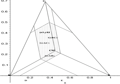
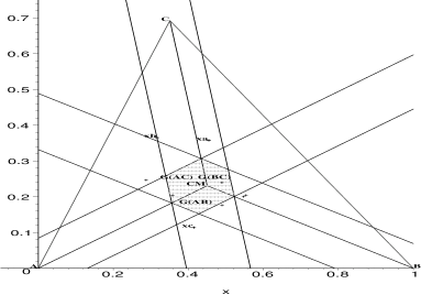
Figure 16: The $\Gamma_{1}$-region $\Gamma_{1}\left(x,N_{CS}^{\tau},M_{C}\right)$ with $x\in R_{M}(e_{2})$ (left) and $\Gamma_{1}\left(X_{n},N_{CS}^{\tau},M_{C}\right)$ with $n>1$ (right).

Remark 6.11.

• For $\tau_{1}<\tau_{2}$, $\Gamma_{1}\left(x,N_{CS}^{\tau_{1}},M\right)\subseteq\Gamma_{1}\left(x,N_{CS}^{\tau_{2}},M\right)$ for all $x\in T\left(\mathcal{Y}_{3}\right)$ with equality holding only when $x\in\partial(T\left(\mathcal{Y}_{3}\right))$.

• Let $\mathcal{X}_{n}$ be a set of $n$ points in $T\left(\mathcal{Y}_{3}\right)$. Then for $\tau_{1}<\tau_{2}$, $\Gamma_{1}\left(\mathcal{X}_{n},N_{CS}^{\tau_{1}},M\right)\subseteq\Gamma_{1}\left(\mathcal{X}_{n},N_{CS}^{\tau_{2}},M\right)$ with equality holding only when $\mathcal{X}_{n}\subset\partial(T\left(\mathcal{Y}_{3}\right))$.

• Suppose $X,Y$ are iid from a continuous distribution $F$ whose support is $\mathcal{S}(F)\subseteq T\left(\mathcal{Y}_{3}\right)$. Then for $\tau_{1}<\tau_{2}$, $A\left(\Gamma_{1}\left(X,N_{CS}^{\tau_{1}},M\right)\right)\leq^{ST}A\left(\Gamma_{1}\left(Y,N_{CS}^{\tau_{2}},M\right)\right)$.

• Suppose $\mathcal{X}_{n}$ and $\mathcal{X}^{\prime}_{n}$ are two random samples from a continuous distribution $F$ whose support is $\mathcal{S}(F)\subseteq T\left(\mathcal{Y}_{3}\right)$. Then for $\tau_{1}<\tau_{2}$, $A(\Gamma_{1}\left(\mathcal{X}_{n},N_{CS}^{\tau_{1}},M\right))\leq^{ST}A(\Gamma_{1}\left(\mathcal{X}^{\prime}_{n},N_{CS}^{\tau_{2}},M\right))$. $\square$

7 Investigation of the Proximity Regions and the Associated PCDs Using the Auxiliary Tools

7.1 Characterization of Proximity Maps Using $\eta$-Values

By definition, it is trivial to show that that the minimum number of points to describe the $\Gamma_{1}$-region, $\eta_{n}(N)\leq n$ for any proximity map. We have improved the upper bound for $N_{PE}^{r}$ and $N_{CS}^{\tau}$: $\eta(\mathcal{X}_{n},N_{PE}^{r})\leq 3$ and $\eta(\mathcal{X}_{n},N_{CS}^{\tau})\leq 3$. However, finding such an improvement does not hold for $\eta_{n}(N_{AS})$; that is, finding a $k<n$ such that $\eta_{n}(N_{AS})\leq k$ for all $\mathcal{X}_{n}$ is still an open problem.

Below we state a condition for $N(\cdot,M)$ defined with $M$-vertex regions to have $\eta_{n}(N)\leq 3$ for $\mathcal{X}_{n}$ with support in $T\left(\mathcal{Y}_{3}\right)$.

Theorem 7.1.

Suppose $N(\cdot,M)$ is a proximity region defined with $M$-vertex regions and $B$ is a set of $n$ distinct points in $T\left(\mathcal{Y}_{3}\right)$. Then $\eta(B,N)\leq 3$ if

• for each $\mathsf{y}_{i}\in\mathcal{Y}_{3}$ there exists a point $x(\mathsf{y}_{i})\in B$ (i.e., related to $\mathsf{y}_{i}$) such that $\Gamma_{1}(B,N)\cap R_{M}(\mathsf{y}_{i})=\Gamma_{1}\left(x(\mathsf{y}_{i}),N\right)\cap R_{M}(\mathsf{y}_{i})$,

• or

• there exist points $x(\mathsf{y}_{j}),\,x(\mathsf{y}_{k})\in B$ such that $\Gamma_{1}(B,N)\cap R_{M}(\mathsf{y}_{i})=\Gamma_{1}\left(x(\mathsf{y}_{j}),N\right)\cap\Gamma_{1}\left(x(\mathsf{y}_{k}),N\right)\cap R_{M}(\mathsf{y}_{i})$ for $j,k\not=i$ with $i\in\{1,2,3\}$ and $(j,k)\in\{(1,2),(1,3),(2,3)\}$.

Proof: Let $B=\{x_{1},x_{2},\ldots,x_{n}\}\subset T\left(\mathcal{Y}_{3}\right)$.

• Suppose there exists a point $x(\mathsf{y}_{i})\in B$ such that $\Gamma_{1}(B,N)\cap R_{M}(\mathsf{y}_{i})=\Gamma_{1}\left(x(\mathsf{y}_{i}),N\right)\cap R_{M}(\mathsf{y}_{i})$ for each $i\in\{1,2,3\}$. Then

  $$\Gamma_{1}(B,N)\cap R_{M}(\mathsf{y}_{i})=\Gamma_{1}\left(x(\mathsf{y}_{i}),N\right)\cap R_{M}(\mathsf{y}_{i})=\\ \bigcap_{i=1}^{n}[\Gamma_{1}\left(x_{i},N\right)\cap R_{M}(\mathsf{y}_{i})]=\bigcap_{j=1}^{3}[\Gamma_{1}\left(x(\mathsf{y}_{j}),N\right)\cap R_{M}(\mathsf{y}_{i})]=\left[\bigcap_{j=1}^{3}\Gamma_{1}\left(x(\mathsf{y}_{j}),N\right)\right]\cap R_{M}(\mathsf{y}_{i})$$

  and

  $$\Gamma_{1}(B,N)=\bigcup_{i=1}^{3}[\Gamma_{1}(B,N)\cap R_{M}(\mathsf{y}_{i})]=\bigcup_{i=1}^{3}\left(\left[\bigcap_{j=1}^{3}\Gamma_{1}\left(x(\mathsf{y}_{j}),N\right)\right]\cap R_{M}(\mathsf{y}_{i})\right).$$

  Then, we get

  $$\Gamma_{1}(B,N)=\bigcap_{i=1}^{3}\Gamma_{1}\left(x(\mathsf{y}_{i}),N\right).$$

  Hence, the minimum active set $S_{M}\subseteq\{x(\mathsf{y}_{1}),x(\mathsf{y}_{2}),x(\mathsf{y}_{3})\}$, which implies $\eta(B,N)\leq 3$. The $\eta$-value $\eta(B,N)<3$ will hold if $x(\mathsf{y}_{i})$ are not all distinct.

• Suppose there exist points $x(\mathsf{y}_{j})$ and $x(\mathsf{y}_{k})$ such that $\Gamma_{1}\left(B,N\right)\cap R_{M}(\mathsf{y}_{i})=\Gamma_{1}\left(x(\mathsf{y}_{j}),N\right)\cap\Gamma_{1}\left(x(\mathsf{y}_{k}),N\right)\cap R_{M}(\mathsf{y}_{i})$ for $j,k\not=i$. Then

  $$\Gamma_{1}\left(B,N\right)\cap R_{M}(\mathsf{y}_{i})=\Gamma_{1}\left(x(\mathsf{y}_{j}),N\right)\cap\Gamma_{1}\left(x(\mathsf{y}_{k}),N\right)\cap R_{M}(\mathsf{y}_{i})=\\ \bigcap_{i=1}^{n}[\Gamma_{1}\left(x_{i},N\right)\cap R_{M}(\mathsf{y}_{i})]=\bigcap_{q=1}^{3}[\Gamma_{1}\left(x(\mathsf{y}_{q}),N\right)\cap R_{M}(\mathsf{y}_{i})]=\left[\bigcap_{q=1}^{3}\Gamma_{1}\left(x(\mathsf{y}_{q}),N\right)\right]\cap R_{M}(\mathsf{y}_{i})$$

  and

  $$\Gamma_{1}(B,N)=\bigcup_{i=1}^{3}[\Gamma_{1}(B,N)\cap R_{M}(\mathsf{y}_{i})]=\bigcup_{i=1}^{3}\left(\left[\bigcap_{q=1}^{3}\Gamma_{1}\left(x(\mathsf{y}_{q}),N\right)\right]\cap R_{M}(\mathsf{y}_{i})\right).$$

  Then, we get $\Gamma_{1}(B,N)=\bigcap_{i=1}^{3}\Gamma_{1}\left(x(\mathsf{y}_{i}),N\right).$ Hence, the minimum active set $S_{M}\subseteq\{x(\mathsf{y}_{1}),x(\mathsf{y}_{2}),x(\mathsf{y}_{3})\}$ which implies $\eta(B,N)\leq 3$. $\blacksquare$

Notice that $N_{PE}^{r}$ satisfies condition (i) Theorem 7.1.

Below we state some conditions for $N(\cdot,M)$ defined with $M$-edge regions to have $\eta$-value less than equal to 3.

Theorem 7.2.

Suppose $N(\cdot,M)$ is a proximity region defined with $M$-edge regions and $B$ is set of $n$ distinct points in $T\left(\mathcal{Y}_{3}\right)$. Then $\eta(B,N)\leq 3$ if

• for each $e_{i}\in\{e_{1},e_{2},e_{3}\}$, there exists a point $x(e_{i})\in B$ such that $\Gamma_{1}(B,N)\cap R_{M}(e_{i})=\Gamma_{1}\left(x(e_{i}),N\right)\cap R_{M}(e_{i})$,

• or

• there exist points $x(e_{j}),\,x(e_{k})\in B$ such that $\Gamma_{1}(B,N)\cap R_{M}(e_{i})=\Gamma_{1}\left(x(e_{j}),N\right)\cap\Gamma_{1}\left(x(e_{k}),N\right)\cap R_{M}(e_{i})$ for $j,k\not=i$ with $i\in\{1,2,3\}$ and $(j,k)\in\{(1,2),(1,3),(2,3)\}$.

Proof: Let $B=\{x_{1},x_{2},\ldots,x_{n}\}\subset T\left(\mathcal{Y}_{3}\right)$.

• Suppose there exists a point $x(e_{i})\in B$ such that $\Gamma_{1}(B,N)\cap R_{M}(e_{i})=\Gamma_{1}\left(x(e_{i}),N\right)\cap R_{M}(e_{i})$ for each $i\in\{1,2,3\}$. Then

  $$\Gamma_{1}(B,N)\cap R_{M}(e_{i})=\Gamma_{1}\left(x(e_{i}),N\right)\cap R_{M}(e_{i})=\\ \bigcap_{i=1}^{n}[\Gamma_{1}\left(x_{i},N\right)\cap R_{M}(e_{i})]=\bigcap_{j=1}^{3}[\Gamma_{1}\left(x(e_{j}),N\right)\cap R_{M}(e_{i})]=\left[\bigcap_{j=1}^{3}\Gamma_{1}\left(x(e_{j}),N\right)\right]\cap R_{M}(e_{i})$$

  and

  $$\Gamma_{1}(B,N)=\bigcup_{i=1}^{3}[\Gamma_{1}(B,N)\cap R_{M}(e_{i})]=\bigcup_{i=1}^{3}\left(\left[\bigcap_{j=1}^{3}\Gamma_{1}\left(x(e_{j}),N\right)\right]\cap R_{M}(e_{i})\right).$$

  Then, we get

  $$\Gamma_{1}\left(\mathcal{X}_{n},N\right)=\bigcap_{j=1}^{3}\Gamma_{1}\left(x(e_{j}),N\right).$$

  Hence, the minimum active set $S_{M}\subseteq\{x(e_{1}),x(e_{2}),x(e_{3})\}$ which implies $\eta_{n}(N)\leq 3$.

• Suppose there exist points $x(e_{j})$ and $x(e_{k})$ such that $\Gamma_{1}\left(\mathcal{X}_{n},N\right)\cap R_{M}(e_{i})=\Gamma_{1}\left(x(e_{j}),N\right)\cap\Gamma_{1}\left(x(e_{k}),N\right)\cap R_{M}(e_{i})$ for $j,k\not=i$. Then

  $$\Gamma_{1}\left(B,N\right)\cap R_{M}(e_{i})=\Gamma_{1}\left(x(e_{j}),N\right)\cap\Gamma_{1}\left(x(e_{k}),N\right)\cap R_{M}(e_{i})=\\ \bigcap_{i=1}^{n}[\Gamma_{1}\left(x_{i},N\right)\cap R_{M}(e_{i})]=\bigcap_{q=1}^{3}[\Gamma_{1}\left(x(e_{q}),N\right)\cap R_{M}(e_{i})]=\left[\bigcap_{q=1}^{3}\Gamma_{1}\left(x(e_{q}),N\right)\right]\cap R_{M}(e_{i})$$

  and

  $$\Gamma_{1}(B,N)=\bigcup_{i=1}^{3}[\Gamma_{1}(B,N)\cap R_{M}(e_{i})]=\bigcup_{i=1}^{3}\left(\left[\bigcap_{q=1}^{3}\Gamma_{1}\left(x(e_{q}),N\right)\right]\cap R_{M}(e_{i})\right).$$

  Then, we get $\Gamma_{1}(B,N)=\bigcap_{i=1}^{3}\Gamma_{1}\left(x(e_{i}),N\right).$ Hence, the minimum active set $S_{M}\subseteq\{x(e_{1}),x(e_{2}),x(e_{3})\}$ which implies $\eta(B,N)\leq 3$. $\blacksquare$

Notice that $N_{CS}^{\tau}$ satisfies condition (ii) in Theorem 7.2.

7.2 The Behavior of $\Gamma_{1}\left(\mathcal{X}_{n},N\right)$ for the Proximity Maps in $T\left(\mathcal{Y}_{3}\right)$

In Section 4, we have investigated the behavior of $\Gamma_{1}\left(\mathcal{X}_{n},N\right)$ for general proximity maps in $\Omega$. The assertions made about $\Gamma_{1}$-regions will be stronger for the proximity regions we have defined, i.e., for $N_{AS}$, $N_{PE}^{r}$, and $N_{CS}^{\tau}$, compared to the general assertions in Section 4. One property enjoyed by these proximity maps is that the region $N(x)$ gets larger as $x$ moves along a line from $\partial(T\left(\mathcal{Y}_{3}\right))$ to $\mathscr{R}_{S}(N)$ in a region with positive $\mathbb{R}^{2}$-Lebesgue measure. So the modifications of the assertions in Section 4 also hold for $\left\{N_{S},N_{AS},N_{PE}^{r},N_{CS}^{\tau}\right\}$. In particular, we have a stronger result than the one in Proposition 4.1 in the sense that, $\mathscr{R}_{S}(N)$ is a proper subset of $\Gamma_{1}\left(\mathcal{X}_{n},N\right)$ as shown below.

Proposition 7.3.

For each type of proximity map $N\in\left\{N_{S},N_{AS},N_{PE}^{r},N_{CS}^{\tau}\right\}$ and any random sample $\mathcal{X}_{n}=\bigl{\{}X_{1},X_{2},\ldots,X_{n}\bigr{\}}$ from a continuous distribution $F$ on $T\left(\mathcal{Y}_{3}\right)$, if $\mathscr{R}_{S}(N)\not=\emptyset$, then $\mathscr{R}_{S}(N)\subsetneq\Gamma_{1}\left(\mathcal{X}_{n},N\right)$ a.s. for each $n<\infty$.

Proof: We have shown that $\mathscr{R}_{S}(N)\subseteq\Gamma_{1}\left(\mathcal{X}_{n},N\right)$ (see Proposition 4.1). Moreover, $\mathscr{R}_{S}(N)\not=\emptyset$ for $N_{AS}$, $N_{PE}^{r}$ with $r>3/2$, and $N_{CS}^{\tau=1}$. For these proximity regions, $\mathscr{R}_{S}(N)=\Gamma_{1}\left(\mathcal{X}_{n},N\right)$ with probability 0 for each finite $n$ since

• for $N\in\left\{N_{S},N_{AS}\right\}$, $\Gamma_{1}\left(\mathcal{X}_{n},N\right)=\mathscr{R}_{S}\left(N\right)$ iff $X_{\mathsf{y}}(n)=\mathsf{y}$ for each $\mathsf{y}\in\mathcal{Y}_{3}$ which happens with probability 0,

• for $N\in\left\{N_{CS}^{\tau=1},\,N_{PE}^{r>3/2}\right\}$, $\Gamma_{1}\left(\mathcal{X}_{n},N,M\right)=\mathscr{R}_{S}\left(N,M\right)$ iff $X_{e_{i}}(n)\in e_{i}$ for each $i\in\{1,2,3\}$ which happens with probability 0.

Furthermore, for $N_{PE}^{r}$ with $r<3/2$, $\mathscr{R}_{S}\left(N_{PE}^{r},M\right)\not=\emptyset$ iff $M\notin(\mathscr{T}^{r})^{o}$ (see Equation (3) for $\mathscr{T}^{r}$), say $M=(m_{x},m_{y})$ is such that $d(\zeta(m_{x},\mathsf{y}_{2}),\mathsf{y}_{2})<d(\mathsf{y}_{2},e_{2})/r$. Then $\Gamma_{1}\left(\mathcal{X}_{n},N_{PE}^{r},M\right)=\mathscr{R}_{S}\left(N_{PE}^{r},M\right)$ iff $X_{e_{2}}(n)\in e_{2}$ which happens with probability 0. Similarly the same result also holds for edges $e_{1}$ and $e_{3}$. $\blacksquare$

Note that, if $\mathscr{R}_{S}(N)=\emptyset$ and $\mathcal{X}_{n}$ is a random sample from a continuous distribution on $T\left(\mathcal{Y}_{3}\right)$, then $\Gamma_{1}\left(\mathcal{X}_{n},N\right)=\emptyset$ a.s. as $n\rightarrow\infty$. In particular, this holds for $N_{PE}^{r}(\cdot,M)$ with $r<3/2$ and $M\in(\mathscr{T}^{r})^{o}$. Lemma 4.6 holds as stated. In Lemma 4.6, we have shown that $\Gamma_{1}\left(\mathcal{X}(n),N\right)$ is non-increasing. Furthermore, for the proximity regions $\left\{N_{S},N_{AS},N_{PE}^{r},N_{CS}^{\tau}\right\}$, we can state that $\Gamma_{1}\left(\mathcal{X}(n+1),N\right)\subsetneq\Gamma_{1}\left(\mathcal{X}(n),N\right)$ with positive probability, since the new point in $\mathcal{X}(n+1)$ has positive probability to fall closer to the subset of $T\left(\mathcal{Y}_{3}\right)$ that defines $\mathscr{R}_{S}(N)$ (e.g., $\partial(T\left(\mathcal{Y}_{3}\right))$). The general results in Theorems 4.8 and 4.10 and Proposition 4.9 hold for the proximity maps $\left\{N_{S},N_{AS},N_{PE}^{r},N_{CS}^{\tau}\right\}$ also. In particular we have the following corollaries to these results.

Corollary to Theorem 4.8: Given a sequence of random variables $X_{1},X_{2},\ldots\stackrel{{\scriptstyle iid}}{{\sim}}\mathcal{U}(T\left(\mathcal{Y}_{3}\right))$, let $\mathcal{X}(n):=\mathcal{X}(n-1)\cup\{X_{n}\}$ for $n=0,1,2,\ldots$ with $\mathcal{X}(0):=\emptyset$. Then for each $N\in\left\{N_{S},N_{AS},N_{PE}^{r},N_{CS}^{\tau}\right\}$, $\Gamma_{1}\left(\mathcal{X}(n),N\right)\downarrow\mathscr{R}_{S}(N)$ as $n\rightarrow\infty$ a.s., in the sense that $\Gamma_{1}\left(\mathcal{X}(n+1),N\right)\subseteq\Gamma_{1}\left(\mathcal{X}(n),N\right)$ and $A(\Gamma_{1}\left(\mathcal{X}(n),N\right)\setminus\mathscr{R}_{S}(N))\downarrow 0$ a.s.

Corollary to Proposition 4.9: For positive integers $m>n$, let $\mathcal{X}_{m}$ and $\mathcal{X}_{n}$ be two random samples from $\mathcal{U}(T\left(\mathcal{Y}_{3}\right))$. Then $A\left(\Gamma_{1}\left(\mathcal{X}_{m},N,M\right)\right)\leq^{ST}A\left(\Gamma_{1}\left(\mathcal{X}_{n},N,M\right)\right)$ for proximity maps $N\in\left\{N_{PE}^{r},N_{CS}^{\tau}\right\}$, for $r\in[1,\infty)$ and $\tau\in(0,1]$.

For $N\in\left\{N_{S},N_{AS}\right\}$, the stochastic ordering of $A\left(\Gamma_{1}\left(\mathcal{X}_{n},N,M\right)\right)$ is still an open problem, although we conjecture that $A\left(\Gamma_{1}\left(\mathcal{X}_{m},N,M\right)\right)\leq^{ST}A\left(\Gamma_{1}\left(\mathcal{X}_{n},N,M\right)\right)$ for $\mathcal{X}_{m}$ and $\mathcal{X}_{n}$ two random samples from $\mathcal{U}(T\left(\mathcal{Y}_{3}\right))$ with $m>n$.

Corollary to Theorem 4.10: Let $\{\mathcal{X}_{n}\}_{n=1}^{\infty}$ be a sequence of data sets which are iid $\mathcal{U}(T\left(\mathcal{Y}_{3}\right))$. Then $\Gamma_{1}\left(\mathcal{X}_{n},N\right)\xrightarrow{a.s.}\mathscr{R}_{S}(N)$ as $n\rightarrow\infty$ for $N\in\left\{N_{S},N_{AS},N_{PE}^{r},N_{CS}^{\tau}\right\}$.

7.3 Expected Measure of $\Gamma_{1}$-Regions

Let $\lambda(\cdot)$ be the $\mathbb{R}^{d}$-Lebesgue measure on $\mathbb{R}^{d}$ with $d\geq 1$. In $\mathbb{R}$, $\lambda(\cdot)$ is the length $|\cdot|$, in $\mathbb{R}^{2}$, $\lambda(\cdot)$ is the area $A(\cdot)$, and in $\mathbb{R}^{d}$, $\lambda(\cdot)$ is the $d$-dimensional volume $V(\cdot)$. In $\mathbb{R}$ with $\mathcal{Y}_{2}=\{0,1\}$, let $\mathcal{X}_{n}$ be a random sample from $\mathcal{U}(0,1)$, and $N_{S}(x)=B(x,r(x))$ where $r(x)=\min(x,1-x)$. Then,

$$\Gamma_{1}\left(\mathcal{X}_{n},N_{S}\right)=\left[X_{n:n}/2,(1+X_{1:n})/2\right]\Longrightarrow\lambda(\Gamma_{1}\left(\mathcal{X}_{n},N_{S}\right))=|\Gamma_{1}\left(\mathcal{X}_{n},N_{S}\right)|=\left(1+X_{1:n}-X_{n:n}\right)/2.$$

Hence the expected length of the $\Gamma_{1}$-region is

$$\mathbf{E}\,[\lambda(\Gamma_{1}\left(\mathcal{X}_{n},N_{S}\right)] = \mathbf{E}\,\left[\frac{1+X_{1:n}-X_{n:n}}{2}\right]=\frac{1+\mathbf{E}\,[X_{1:n}]-\mathbf{E}\,[X_{n:n}]}{2}$$

$$= \frac{1+\frac{1}{n+1}-\frac{n}{n+1}}{2}=\frac{1}{n+1}\rightarrow 0\text{ as }n\rightarrow\infty.$$

In $\mathbb{R}^{2}$, with three non-collinear points $\mathcal{Y}_{3}=\{\mathsf{y}_{1},\mathsf{y}_{2},\mathsf{y}_{3}\}$, let $\mathcal{X}_{n}$ be a random sample from $\mathcal{U}(T\left(\mathcal{Y}_{3}\right))$. Then $A(\Gamma_{1}\left(\mathcal{X}_{n},N_{PE}^{r},M\right))>0$ a.s. for all $n<\infty$, $r>3/2$, $M\in\mathbb{R}^{2}\setminus\mathcal{Y}_{3}$. Furthermore, $A(\Gamma_{1}\left(\mathcal{X}_{n},N_{CS}^{\tau=1},M\right))>0$ a.s. for all $n<\infty$ and $M\in(T\left(\mathcal{Y}_{3}\right))^{o}$; and for $N\in\left\{N_{S},N_{AS}\right\}$ $A(\Gamma_{1}\left(\mathcal{X}_{n},N,M\right))>0$ a.s. for all $n<\infty$ and $M\in\mathbb{R}^{2}\setminus\mathcal{Y}_{3}$.

The $\Gamma_{1}$-region, $\Gamma_{1}\left(\mathcal{X}_{n},N\right)$, is closely related to the distribution of the domination number of the PCD associated with $N$. Hence we study the asymptotic behavior of the expected area $\mathbf{E}\,[A(\Gamma_{1}\left(\mathcal{X}_{n},N,M\right)]$, as $n\rightarrow\infty$, for $N\in\left\{N_{AS},N_{PE}^{r},N_{CS}^{\tau}\right\}$.

In $\mathbb{R}$, $N_{S}$ and $N_{AS}$ are equivalent functions, with the extension that $N_{AS}$ is defined as $N_{S}$ for $\mathcal{X}$ points outside $(\mathsf{y}_{1:m},\mathsf{y}_{m:m})$. In higher dimensions, determining the areas of $\Gamma_{1}\left(\mathcal{X}_{n},N,M\right)$ for for $N\in\left\{N_{S},N_{AS}\right\}$ and for general $\mathcal{X}_{n}$ and hence finding its expected areas are both open problems.

7.3.1 The Limit of Expected Area of $\Gamma_{1}\left(\mathcal{X}_{n},N,M\right)$ for $N_{PE}^{r}$ and $N_{CS}^{\tau}$

Recall that for $N\in\{N_{PE}^{r},\,N_{CS}^{\tau}\}$, $\Gamma_{1}\left(\mathcal{X}_{n},N,M\right)$ is determined by the (closest) edge extrema $X_{e}(n)\in\operatorname{argmin}_{X\in\mathcal{X}_{n}}d(X,e)$, for $e\in\{e_{1},e_{2},e_{3}\}$. So, to find the expected area of $\Gamma_{1}\left(\mathcal{X}_{n},N,M\right)$, we need to find the expected locus of $X_{e}(n)$; i.e., the expected distance of $d(X_{e}(n)$ from $e$. For example, for $\mathcal{X}_{n}$ a random sample from a continuous distribution $F$, $\operatorname{argmin}_{X\in\mathcal{X}_{n}}d(X,e)$ is unique a.s., and if $d(X_{e}(n),e)=u$, then $X_{e}(n)$ falls on a line parallel to $e$ whose distance from $e$ is $u$ a.s.

Lemma 7.4.

Let $D_{i}(n):=d(X_{e_{i}}(n),e_{i})$ for $i\in\{1,2,3\}$ and $\mathcal{X}_{n}$ be a random sample from $\mathcal{U}(T\left(\mathcal{Y}_{3}\right))$. Then $\mathbf{E}\,[D_{i}(n)]\rightarrow 0$ (i.e., the expected locus of $X_{e_{i}}(n)$ is on $e_{i}$) for each $i\in\{1,2,3\}$, as $n\rightarrow\infty$.

Proof: Given $Z_{i}=(X_{i},Y_{i})\stackrel{{\scriptstyle iid}}{{\sim}}\mathcal{U}(T\left(\mathcal{Y}_{3}\right))$. Then for $e=e_{3}$, $D_{3}(n)=Y_{1:n}$ (the minimum $y$-coordinate of $Z_{i}\in\mathcal{X}_{n}$). First observe that $\displaystyle P(Y_{i}\leq y)={\frac{y\,(2\,c_{2}-y)}{c_{2}^{2}}}$, hence

$$F_{Y}(y)={\frac{y\,(2\,c_{2}-y)}{c_{2}^{2}}}\mathbf{I}(0\leq y<c_{2})+\mathbf{I}(y\geq c_{2}).$$

So the pdf of $Y_{i}$ is $\displaystyle f_{Y}(y)=2\,{\frac{c_{2}-y}{c_{2}^{2}}}\mathbf{I}(0\leq y\leq c_{2})$. Then the pdf of $Y_{1:n}$ is

$$f_{1:n}(y)=2\,n(c_{2}-y)\left(1-{\frac{y\,(2\,c_{2}-y)}{c_{2}^{2}}}\right)^{n-1}{c_{2}}^{-2}\mathbf{I}(0\leq y\leq c_{2}).$$

Therefore,

$$\mathbf{E}\,\,[Y_{1:n}]=\int_{0}^{c_{2}}\!2\,y\,n(c_{2}-y)\left(1-{\frac{y\,(2\,c_{2}-y)}{c_{2}^{2}}}\right)^{n-1}{c_{2}}^{-2}{dy}=\frac{c_{2}}{2\,n+1}\rightarrow 0,\text{ as }n\rightarrow\infty.$$

Hence $\mathbf{E}\,[Y_{1:n}]=\mathbf{E}\,[D_{3}(n)]\rightarrow 0$. Similarly, $\mathbf{E}\,[D_{i}(n)]\rightarrow 0$ for $i\in\{1,2\},$ as $n\rightarrow\infty$. $\blacksquare$

Theorem 7.5.

Let $\mathcal{X}_{n}$ be a random sample from $\mathcal{U}(T\left(\mathcal{Y}_{3}\right))$ and $M\in T\left(\mathcal{Y}_{3}\right)^{o}$. For $N\in\{N_{PE}^{r},\,N_{CS}^{\tau}\}$, $\mathbf{E}\,[A(\Gamma_{1}\left(\mathcal{X}_{n},N,M\right))]\rightarrow A(\mathscr{R}_{S}(N,M))$ as $n\rightarrow\infty$.

Proof: Recall that for $N\in\{N_{PE}^{r},\,N_{CS}^{\tau}\}$, $\Gamma_{1}\left(\mathcal{X}_{n},N,M\right)=\bigcap_{i=1}^{3}\Gamma_{1}\left(X_{e_{i}}(n),N,M\right)$. Moreover, $\Gamma_{1}\left(\mathcal{X}_{n},N,M\right)=\mathscr{R}_{S}(N,M)$ iff $X_{e_{i}}(n)\in e_{i}$ for $i\in\{1,2,3\}$. In Lemma 7.4, we have shown that expected locus of $X_{e}(n)$ converges to edge $e$ as $n\rightarrow\infty$. Hence the expected locus of $\partial(\Gamma_{1}\left(\mathcal{X}_{n},N,M\right))\cap R_{M}(e_{i})$ converges to the $\partial(\mathscr{R}_{S}(N,M))\cap R_{M}(e_{i})$ for each $i\in\{1,2,3\}$. Hence

$$\mathbf{E}\,[A(\Gamma_{1}\left(\mathcal{X}_{n},N,M\right)]\rightarrow A(\mathscr{R}_{S}(N,M))\text{ as }n\rightarrow\infty.\;\blacksquare$$

Remark 7.6.

In particular,

• $\mathbf{E}\,\left[A\left(\Gamma_{1}\left(\mathcal{X}_{n},N_{PE}^{2},M_{C}\right)\right)\right]\rightarrow 1/4$ as $n\rightarrow\infty$, since $\mathscr{R}_{S}\left(N_{PE}^{2},M_{C}\right)=T(M_{1},M_{2},M_{3})$.

• $\mathbf{E}\,\left[A\left(\Gamma_{1}\left(\mathcal{X}_{n},N_{PE}^{r},M\right)\right)\right]\rightarrow 0$ as $n\rightarrow\infty$ if $M\in\mathscr{T}^{r}$, since $\mathscr{R}_{S}\left(N_{PE}^{r},M\right)=\emptyset$ for $M\in\mathscr{T}^{r}$.

• Furthermore, $\mathbf{E}\,\left[A\left(\Gamma_{1}\left(\mathcal{X}_{n},N_{PE}^{3/2},M_{C}\right)\right)\right]\rightarrow 0$ since $\mathscr{R}_{S}\left(N_{PE}^{3/2},M_{C}\right)=\{M_{C}\}$.

• For any $M\in T\left(\mathcal{Y}_{3}\right)^{o}$, $\mathbf{E}\,\left[A\left(\Gamma_{1}\left(\mathcal{X}_{n},N_{CS}^{\tau},M)\right)\right)\right]\rightarrow 0$ as $n\rightarrow\infty$, since $\mathscr{R}_{S}\left(N^{\tau}_{CS},M\right)=\{M\}$.

• We also have $\mathbf{E}\,\left[A\left(\Gamma_{1}\left(\mathcal{X}_{n},N_{PE}^{r},M_{C}\right)\right)\right]\rightarrow 0$ for $r\in[1,3/2]$ as $n\rightarrow\infty$.

• Furthermore, by careful geometric calculations, we get $\mathbf{E}\,\left[A\left(\Gamma_{1}\left(\mathcal{X}_{n},N_{PE}^{r},M_{C}\right)\right)\right]\rightarrow\sqrt{3}\left[1-3/(2\,r)\right]^{2}$ for $r\in(3/2,2]$.

• $\mathbf{E}\,\left[A\left(\Gamma_{1}\left(\mathcal{X}_{n},N_{PE}^{r},M_{C}\right)\right)\right]\rightarrow\sqrt{3}/\left[4\,(1-3/r^{2})\right]$ for $r\in(2,\infty]$, as $n\rightarrow\infty$.

We also derive the rate of convergence of $\mathbf{E}\,[A(\Gamma_{1}\left(\mathcal{X}_{n},N_{PE}^{r},M_{C}\right))]$ for $r=3/2$.

Theorem 7.7.

Let $\mathcal{X}_{n}$ be a random sample from $\mathcal{U}(T\left(\mathcal{Y}_{3}\right))$. For $r=3/2$, the expected area of the the $\Gamma_{1}$-region, $\mathbf{E}\,\left[A\left(\Gamma_{1}\left(\mathcal{X}_{n},N_{PE}^{r},M_{C}\right)\right)\right]$, converges to zero, at rate $O\left(n^{-2}\right)$.

Proof: For $r=3/2$ and $M=M_{C}$, and sufficiently large $n$, $\Gamma_{1}\left(X_{e_{i}},N_{PE}^{r}\right)\cap R_{CM}(\mathsf{y}_{i})$ is a triangle for $i=1,2,3$ w.p. 1. See Figure 17. With the realization of the edge extrema denoted as $x_{e_{i}}=(x_{i},y_{i})$ close enough to $e_{i}$, for $i=1,2,3$,

$\Gamma_{1}\left(x_{e_{1}},N_{PE}^{3/2}\right)\cap R_{CM}(\mathsf{y}_{1})$ is the triangle with vertices

$$\left(\frac{\sqrt{3}}{3}\,y_{2}+x_{2}-\frac{1}{2},-\frac{\sqrt{3}}{18}\,\left(-9+2\,\sqrt{3}\,y_{2}+6\,x_{2}\right)\right),\left(\frac{1}{2},\frac{\sqrt{3}}{9}\left(-\frac{9}{2}+2\,\sqrt{3}\,y_{2}+6\,x_{2}\right)\right),\left(\frac{1}{2},\frac{\sqrt{3}}{6}\right),$$

$\Gamma_{1}\left(x_{e_{2}},N_{PE}^{3/2}\right)\cap R_{CM}(\mathsf{y}_{2})$ is the triangle with vertices

$$\left(\frac{1}{2},\frac{\sqrt{3}}{18}\,\left(3+4\,\sqrt{3}\,y_{3}-12\,x_{3}\right)\right),\left(\frac{1}{2}-\frac{\sqrt{3}}{3}\,y_{3}+x_{3},-\frac{\sqrt{3}}{18}\left(-3+2\,\sqrt{3}\,y_{3}-6\,x_{3}\right)\right),\left(\frac{1}{2},\frac{\sqrt{3}}{6}\right),$$

and $\Gamma_{1}\left(x_{e_{3}},N_{PE}^{3/2}\right)\cap R_{CM}(\mathsf{y}_{3})$ is the triangle with vertices

$$\left(-\frac{\sqrt{3}}{6}\,\left(-\sqrt{3}+4\,y_{1}\right),\frac{\sqrt{3}}{6}+\frac{2}{3}\,y_{1}\right),\left(\frac{1}{2},\frac{\sqrt{3}}{6}\right),\left(\frac{\sqrt{3}}{6}\,\left(\sqrt{3}+4\,y_{1}\right),\frac{\sqrt{3}}{6}+\frac{2}{3}\,y_{1}\right).$$

Figure 17: The shaded regions are the triangular $\Gamma_{1}^{3/2}(X_{e_{i}})\cap R_{CM}(\mathsf{y}_{i})$ regions for $i=1,2,3$.

Then for sufficiently large $n$,

$$A\left(\Gamma_{1}\left(\mathcal{X}_{n},N_{PE}^{3/2},M\right)\right)=\frac{\sqrt{3}}{27}\left(3\,x_{2}-3+\sqrt{3}\,y_{2}\right)^{2}+\frac{\sqrt{3}}{27}\left(-3\,x_{3}+\sqrt{3}\,y_{3}\right)^{2}+\frac{4\,\sqrt{3}}{9}y_{1}^{2}$$

$$=\frac{\sqrt{3}}{9}\left(3\,x_{2}^{2}-6\,x_{2}+2\,\sqrt{3}\,y_{2}\,x_{2}-2\,\sqrt{3}\,y_{2}+y_{2}^{2}+3+y_{3}^{2}-2\,\sqrt{3}\,y_{3}\,x_{3}+3\,x_{3}^{2}+4\,y_{1}^{2}\right).$$

To find the expected area, we need the joint density of the $X_{e_{i}}$. The edge extrema are all distinct with probability 1 as $n\rightarrow\infty$ (see Theorem 6.4). Let $T(\zeta)$ be the triangle formed by the lines at $x_{e_{i}}$ parallel to $e_{i}$ for $i=1,2,3$ where $\zeta=(x_{1},y_{1},x_{2},y_{2},x_{3},y_{3})$. See Figure 18.

Figure 18: The figure for the joint pdf of $X_{e_{i}}$. The shaded region is $T(\zeta)$.

Then the asymptotically accurate joint pdf of $X_{e_{i}}$ (Ceyhan and Priebe, (2007)) is

$$f_{3}(\zeta) = n(n-1)(n-2)\left(\frac{A(T(\zeta))}{A(T\left(\mathcal{Y}_{3}\right))}\right)^{n-3}\frac{1}{A(T\left(\mathcal{Y}_{3}\right))^{3}}$$

$$= n(n-1)(n-2)\left(\sqrt{3}/36\left(-2\,\sqrt{3}\,y_{1}+\sqrt{3}\,y_{3}-3\,x_{3}+\sqrt{3}\,y_{2}+3\,x_{2}\right)^{2}\right)^{n-3}\Big{/}\left(\sqrt{3}/4\right)^{n}.$$

with the support $D_{S}=\bigl{\{}\zeta\in\Re^{6}:\;(x_{i},y_{i})\text{'s are distinct}\bigr{\}}.$

Then for sufficiently large $n$,

$$\mathbf{E}\,\left[A\left(\Gamma_{1}\left(\mathcal{X}_{n},N_{PE}^{3/2},M\right)\right)\right] \sim \int A\left(\Gamma_{1}\left(\mathcal{X}_{n},N_{PE}^{3/2}\right)\right)f_{3}(\zeta)d\zeta$$

$$= \int A\left(\Gamma_{1}\left(\mathcal{X}_{n},N_{PE}^{3/2}\right)\right)n(n-1)(n-2)\left(\frac{A(T(\zeta))}{A(T\left(\mathcal{Y}_{3}\right))}\right)^{n-3}\frac{1}{A(T\left(\mathcal{Y}_{3}\right))^{3}}d\zeta.$$

Let $G(\zeta)=A(T(\zeta))/A(T\left(\mathcal{Y}_{3}\right))$. Notice that the integrand is critical when $x_{e_{i}}\in e_{i}$ for $i=1,2,3$, since $G(\zeta)$ when $x_{e_{i}}\in e_{i}$ for each $i=1,2,3$. So we make the change of variables $y_{1}=z_{1}$, $y_{2}=\sqrt{3}\,(1-x_{2})-z_{2}$, and $y_{3}=\sqrt{3}\,x_{3}-z_{3}$, then $G(\zeta)$ and $A(\Gamma_{1}\left(\mathcal{X}_{n},N\right))$ becomes

$$G(\zeta)=G(z_{1},z_{2},z_{3})=\left(2\,z_{1}+z_{3}-\sqrt{3}+z_{2}\right)^{2}\Big{/}3\text{ and }A(\Gamma_{1}\left(\mathcal{X}_{n},N\right))=\sqrt{3}\,\left(z_{2}^{2}+z_{3}^{2}+4\,z_{1}^{2}\right)/9,$$

respectively. Hence the integrand does not depend on $x_{1},x_{2},x_{3}$ and integrating with respect to $x_{1},x_{2},x_{3}$ yields a constant $K$. Now, the integrand is critical at $(z_{1},z_{2},z_{3})=(0,0,0)$, since $G(0,0,0)=1$. So let $E^{\varepsilon}_{u}$ be the event that $0\leq z_{i}\leq\varepsilon$ for $i=1,2,3$ for $\varepsilon>0$ small enough. Then making the change of variables $z_{i}=w_{i}/n$ for $i=1,2,3$, we get $A\left(\Gamma_{1}\left(\mathcal{X}_{n},N_{PE}^{3/2}\right)\right)=O\left(n^{-2}\right)$ and $G(z_{1},z_{2},z_{3})$ becomes $G(w_{1},w_{2},w_{3})=1-\frac{1}{n}\left(2/\sqrt{3}\,(2\,w_{1}+w_{2}+w_{3})\right)+O\left(n^{-2}\right)$, hence

$$\mathbf{E}\,\left[A\left(\Gamma_{1}\left(\mathcal{X}_{n},N_{PE}^{3/2},M\right)\right)\right]\sim$$

$$K\int_{0}^{n\varepsilon}\int_{0}^{n\varepsilon}\int_{0}^{n\varepsilon}A\left(\Gamma_{1}\left(\mathcal{X}_{n},N_{PE}^{3/2}\right)\right)n(n-1)(n-2)\frac{1}{n^{3}}\,G(w_{1},w_{2},w_{3})^{n-3}dw_{1}dw_{2}dw_{3},$$

letting $$n\rightarrow\infty$$

$$\approx K\int_{0}^{\infty}\int_{0}^{\infty}\int_{0}^{\infty}O\left(n^{-2}\right)\exp\left(-2/\sqrt{3}\,(2\,w_{1}+w_{2}+w_{3})\right)dw_{1}dw_{2}dw_{3}=O\left(n^{-2}\right),$$

since $\int_{0}^{\infty}\int_{0}^{\infty}\int_{0}^{\infty}\exp\left(-2/\sqrt{3}\,(2\,w_{1}+w_{2}+w_{3})\right)dw_{1}dw_{2}dw_{3}=3\,\sqrt{3}/16$ which is a finite constant. Hence $\mathbf{E}\,\left[A\left(\Gamma_{1}\left(\mathcal{X}_{n},N_{PE}^{3/2},M\right)\right)\right]\rightarrow 0$ as $n\rightarrow\infty$ at the rate $O\left(n^{-2}\right)$. $\blacksquare$

8 $\Gamma_{k}$-Regions for Proximity Maps in $T\left(\mathcal{Y}_{3}\right)$

We can also define the regions associated with $\gamma_{n}(N)=k$ for $k\leq n$.

In $\mathbb{R}$ with $\mathcal{Y}_{2}=\{0,1\}$, $\gamma_{n}(N)\leq 2$, hence we can only define $\Gamma_{2}$-regions. Recall that $\gamma_{n}(N)=2$ iff $\mathcal{X}_{n}\cap\left[\frac{x_{n:n}}{2},\frac{1+x_{1:n}}{2}\right]=\emptyset$ iff $\mathcal{X}_{n}\subset[0,1]\setminus\Gamma_{1}\left(\mathcal{X}_{n},N\right)$. So

$$\Gamma_{2}\left(\mathcal{X}_{n},N\right) = \left\{(x,y)\in[0,1]^{2}:\;\mathcal{X}_{n}\subset N(x)\cup N(y);\;x,y\notin\Gamma_{1}\left(\mathcal{X}_{n},N\right)\right\}$$

$$= \left\{(x,y)\in[0,1]^{2}\setminus\Gamma_{1}\left(\mathcal{X}_{n},N\right)^{2}:\;\mathcal{X}_{n}\subset N(x)\cup N(y)\right\}.$$

Notice that $\Gamma_{2}\left(\mathcal{X}_{n},N\right)\subseteq[0,1]^{2}$. Let

$$\widetilde{x}_{1}:=\operatorname{argmin}_{x\in\mathcal{X}_{n}\cap(0,1/2)}(1/2-x)\text{ and }\widetilde{x}_{2}:=\operatorname{argmin}_{x\in\mathcal{X}_{n}\cap(1/2,1)}(x-1/2),$$

then $\gamma_{n}(N)=2$ iff $\widetilde{x}_{1},\widetilde{x}_{2}\notin\Gamma_{1}\left(\mathcal{X}_{n},N\right)$. In such a case $\mathcal{X}_{n}\subset N(\widetilde{x}_{1})\cup N(\widetilde{x}_{2})$ by construction.

In general,

Definition 8.1.

The $\Gamma_{2}$-region for proximity map $N_{\mathcal{Y}}(\cdot)$ and set $B\subset\Omega$ is $\Gamma_{2}(B,N)=\{(x,y)\in[\Omega\setminus\Gamma_{1}(B)]^{2}:\;B\subseteq N_{\mathcal{Y}}(x)\cup N_{\mathcal{Y}}(y)\}$. In general, $\Gamma_{k}$-region for proximity map $N_{\mathcal{Y}}(\cdot)$ and set $B\subset\Omega$ for $k=1,2,\ldots,n$ is

$$\Gamma_{k}(B,N)=\Biggl{\{}(x_{1},x_{2},\ldots,x_{k})\in\Omega^{k}:B\subseteq\bigcup_{i=1}^{k}N_{\mathcal{Y}}\left(x_{i}\right)\;\text{ and all possible $m$-permutations $(u_{1},u_{2},\ldots,u_{m})$}\\ \text{ of $(x_{1},x_{2},\ldots,x_{k})$ satisfy }(u_{1},u_{2},\ldots,u_{m})\not\in\Gamma_{m}(B,N)\text{ for each }m=1,2,\ldots,k-1\Biggr{\}}.\square$$

Note that $\Gamma_{k}$-regions are defined for $k\leq n$ and they might be empty. Moreover, $\Gamma_{k}$-regions are in $\Omega^{k}$, not in $\Omega$.

Let $\displaystyle\left\{{n\atop m}\right\}$ denote the Stirling partition number for a set of size $n$ into $m$ blocks and let $\left\{{A\atop m}\right\}$ denote all Stirling partitions of a set $A$ into $m$ blocks; that is,

$$\left\{{A\atop m}\right\}:=\left\{\{\mathcal{B}_{1},\mathcal{B}_{2},\ldots,\mathcal{B}_{m}\}:\;\mathcal{B}_{i}\not=\emptyset,\mathcal{B}_{i}\subset A;\;A=\bigcup_{i}\mathcal{B}_{i}\right\}.$$

In particular, $\left\{{\mathcal{X}_{n}\atop 2}\right\}$ is the unordered pair of blocks $\mathcal{B}_{1}$ and $\mathcal{B}_{2}$ such that $\mathcal{B}_{i}\not=\emptyset$ and $\mathcal{B}_{i}\subset\mathcal{X}_{n}$ for $i=1,2$, and $\mathcal{B}_{1}\cup\mathcal{B}_{2}=\mathcal{X}_{n}$. Note that $\mathcal{B}_{2}=\mathcal{X}_{n}\setminus\mathcal{B}_{1}$. Then

Proposition 8.2.

$\Gamma_{2}\left(\mathcal{X}_{n},N\right)=\bigcup_{\{\mathcal{B}_{1},\mathcal{B}_{2}\}\in\left\{{\mathcal{X}_{n}\atop 2}\right\}}[\Gamma_{1}\left(\mathcal{B}_{1},N\right)\times\Gamma_{1}\left(\mathcal{B}_{2},N\right)]\setminus\Gamma_{1}\left(\mathcal{X}_{n},N\right)^{2}$ for any nonempty Stirling blocks $\mathcal{B}_{1}$ and $\mathcal{B}_{2}$ in $\left\{{\mathcal{X}_{n}\atop 2}\right\}$.

Proof: Given $\mathcal{X}_{n}$, suppose $(u,v)\in\Gamma_{2}\left(\mathcal{X}_{n},N\right)$, then $\mathcal{X}_{n}\subset N(u)\cup N(v)$ and $u,v\notin\Gamma_{1}\left(\mathcal{X}_{n},N\right)$. Let $\mathcal{B}_{1}=\mathcal{X}_{n}\cap N(u)$, and $\mathcal{B}_{2}=[\mathcal{X}_{n}\cap N(v)]\setminus N(u)$. Then $\mathcal{B}_{1}$ and $\mathcal{B}_{2}$ are two Stirling blocks in $\left\{{\mathcal{X}_{n}\atop 2}\right\}$. Hence $\mathcal{B}_{1}\subset N(u)\Rightarrow u\in\Gamma_{1}\left(\mathcal{B}_{1},N\right)\setminus\Gamma_{1}\left(\mathcal{X}_{n},N\right)$ and $\mathcal{B}_{2}\subset N(v)\Rightarrow v\in\Gamma_{1}\left(\mathcal{B}_{2},N\right)\setminus\Gamma_{1}\left(\mathcal{X}_{n},N\right)$, hence $\Gamma_{2}\left(\mathcal{X}_{n},N\right)\subseteq\bigcup_{\{\mathcal{B}_{1},\mathcal{B}_{2}\}\in\left\{{\mathcal{X}_{n}\atop 2}\right\}}[\Gamma_{1}\left(\mathcal{B}_{1},N\right)\times\Gamma_{1}\left(\mathcal{B}_{2},N\right)]\setminus(\Gamma_{1}\left(\mathcal{X}_{n},N\right))^{2}$. The other direction is trivial, hence the desired result follows. $\blacksquare$

In $\mathbb{R}$ with $N=N_{S}$, we can exploit the natural ordering available.

Proposition 8.3.

In $\mathbb{R}$ with $\mathcal{Y}_{2}=\{0,1\}$, $\displaystyle\Gamma_{2}\left(\mathcal{X}_{n},N_{S}\right)=\bigcup_{k=1}^{n-1}\left(\frac{x_{k:n}}{2},\frac{x_{n:n}}{2}\right)\times\left(\frac{1+x_{1:n}}{2},\frac{1+x_{(k+1):n}}{2}\right)$.

Proof: Recall that $\Gamma_{2}\left(\mathcal{X}_{n},N_{S}\right)=\bigcup_{\{\mathcal{B}_{1},\mathcal{B}_{2}\}\in\left\{{\mathcal{X}_{n}\atop 2}\right\}}[\Gamma_{1}\left(\mathcal{B}_{1},N_{S}\right)\times\Gamma_{1}\left(\mathcal{B}_{2},N_{S}\right)]\setminus\Gamma_{1}\left(\mathcal{X}_{n},N_{S}\right)^{2}$. Let $\{\mathcal{B}_{1},\mathcal{B}_{2}\}$ be a Stirling partition in $\left\{{\mathcal{X}_{n}\atop 2}\right\}$. First observe that $\mathcal{B}_{1}=\{x_{1:n},\ldots,x_{k:n}\}$ and $\mathcal{B}_{2}=\{x_{(k+1):n},\ldots,x_{n:n}\}$ forms a Stirling partition of $\mathcal{X}_{n}$, and

$$\Gamma_{1}\left(\{x_{1:n},\ldots,x_{k:n}\},N_{S}\right)\setminus\Gamma_{1}\left(\mathcal{X}_{n},N_{S}\right)=\left[\frac{x_{k:n}}{2},\frac{1+x_{1:n}}{2}\right]\setminus\left[\frac{x_{n:n}}{2},\frac{1+x_{1:n}}{2}\right]=\Biggl{[}\frac{x_{k:n}}{2},\frac{x_{n:n}}{2}\Biggr{)}$$

and

$$\Gamma_{1}\left(\{x_{(k+1)},\ldots,x_{n:n}\},N_{S}\right)\setminus\Gamma_{1}\left(\mathcal{X}_{n},N_{S}\right)=\left[\frac{x_{n:n}}{2},\frac{1+x_{(k+1)}}{2}\right]\setminus\left[\frac{x_{n:n}}{2},\frac{1+x_{1:n}}{2}\right]=\Biggl{(}\frac{1+x_{1:n}}{2},\frac{1+x_{(k+1)}}{2}\Biggr{]}.$$

Furthermore,

$$\Gamma_{1}\left(\{x_{1:n},\ldots,x_{k:n}\},N_{S}\right)\times\Gamma_{1}\left(\{x_{(k+1)},\ldots,x_{n:n}\},N_{S}\right)\supseteq\bigcup_{\{\mathcal{B}_{1},\mathcal{B}_{2}\}\in\Lambda}\Gamma_{1}\left(\mathcal{B}_{1},N_{S}\right)\times\Gamma_{1}\left(\mathcal{B}_{2},N_{S}\right)$$ (5)

where

$$\Lambda=\left\{\{\mathcal{B}_{1},\mathcal{B}_{2}\}\in\left\{{\mathcal{X}_{n}\atop 2}\right\}:\;x_{1:n}\in\mathcal{B}_{1},\;x_{n:n}\in\mathcal{B}_{2},\;\max\left(\mathcal{B}_{1}\right)=x_{k:n},\;\min\left(\mathcal{B}_{2}\right)=x_{(l)},\;l<k\right\},$$

since the left hand side in Equation (5) is $\displaystyle\left[\frac{x_{k:n}}{2},\frac{x_{n:n}}{2}\right]\times\left[\frac{1+x_{1:n}}{2},\frac{1+x_{(k-1)}}{2}\right]$. Hence the desired result follows. $\blacksquare$

Similarly, for $N_{PE}^{r}$,

$$\Gamma_{2}\left(\mathcal{X}_{n},N_{PE}^{r}\right)=\bigcup_{\{\mathcal{B}_{1},\mathcal{B}_{2}\}\in\left\{{\mathcal{X}_{n}\atop 2}\right\}}\left[\Gamma_{1}\left(\mathcal{B}_{1},N_{PE}^{r},M\right)\times\Gamma_{1}\left(\mathcal{B}_{2},N_{PE}^{r},M\right)\right]\setminus\Gamma_{1}\left(\mathcal{X}_{n},N_{PE}^{r},M\right)^{2}.$$

Note that $\Gamma_{1}\left(\mathcal{B}_{i},N_{PE}^{r},M\right)$ is determined by the edge extrema in $\mathcal{B}_{i}$, $i=1,2$. Furthermore, if $(u,v)\in\Gamma_{2}\left(\mathcal{X}_{n},N_{PE}^{r},M\right)$, then $(u,v)\notin R_{M}(\mathsf{y})^{2}$, since either $N_{PE}^{r}(u)\subseteq N_{PE}^{r}(v)$ or $N_{PE}^{r}(v)\subseteq N_{PE}^{r}(u)$ should hold if $(u,v)\in R_{M}(\mathsf{y})^{2}$.

For $N_{CS}^{\tau}$,

$$\Gamma_{2}\left(\mathcal{X}_{n},N_{CS}^{\tau},M\right)=\bigcup_{\{\mathcal{B}_{1},\mathcal{B}_{2}\}\in\left\{{\mathcal{X}_{n}\atop 2}\right\}}\left[\Gamma_{1}\left(\mathcal{B}_{1},N_{CS}^{\tau},M\right)\times\Gamma_{1}\left(\mathcal{B}_{2},N_{CS}^{\tau},M\right)\right]\setminus\Gamma_{1}\left(\mathcal{X}_{n},N_{CS}^{\tau},M\right)^{2}.$$

Note that $\Gamma_{1}\left(\mathcal{B}_{i},N_{CS}^{\tau},M\right)$ is determined by the edge extrema of $\mathcal{B}_{i}$, $i=1,2$. But if $(u,v)\in\Gamma_{2}\left(\mathcal{X}_{n},N_{CS}^{\tau},M\right)$, then $(u,v)\in R_{M}(e)^{2}$ can hold. In these proximity regions, not all edge extrema should fall in the same partition set for $\Gamma_{k}\left(\mathcal{X}_{n},N_{CS}^{\tau},M\right)$ to be nonempty.

For any proximity map $N$,

$$P(\gamma_{n}(N)=2)=P(\mathcal{X}_{n}^{2}\cap\Gamma_{2}\left(\mathcal{X}_{n},N\right)\not=\emptyset,\,\gamma_{n}(N)\not=1)$$

$$=P\left(\mathcal{X}_{n}^{2}\bigcap\left[\bigcup_{\{\mathcal{B}_{1},\mathcal{B}_{2}\}\in\left\{{\mathcal{X}_{n}\atop 2}\right\}}\left[\Gamma_{1}\left(\mathcal{B}_{1},N\right)\times\Gamma_{1}\left(\mathcal{B}_{2},N\right)\right]\setminus(\Gamma_{1}\left(\mathcal{X}_{n},N\right))^{2}\right]\not=\emptyset,\,\mathcal{X}_{n}\cap\Gamma_{1}\left(\mathcal{X}_{n},N\right)=\emptyset\right).$$

A more compact way to write this is as

$$P(\gamma_{n}(N)>2)=P\left(\mathcal{X}_{n}^{2}\cap\Gamma_{\leq 2}\left(\mathcal{X}_{n},N\right)=\emptyset\right)$$

where $\Gamma_{\leq 2}\left(\mathcal{X}_{n},N\right):=\bigcup_{\{\mathcal{B}_{1},\mathcal{B}_{2}\}\in\left\{{\mathcal{X}_{n}\atop 2}\right\}}\Gamma_{1}\left(\mathcal{B}_{1},N\right)\times\Gamma_{1}\left(\mathcal{B}_{2},N\right)$.

Furthermore, for $k\geq 3$, the $\Gamma_{k}$-regions are defined similarly as

$$\Gamma_{k}\left(\mathcal{X}_{n},N\right)=\bigcup_{\{\mathcal{B}_{1},\ldots,\mathcal{B}_{k}\}\in\left\{{\mathcal{X}_{n}\atop k}\right\}}[\Gamma_{1}\left(\mathcal{B}_{1},N\right)\times\ldots\times\Gamma_{1}\left(\mathcal{B}_{k},N\right)]\setminus\Gamma_{1}\left(\mathcal{X}_{n},N\right)^{k}.$$

Hence,

$$P(\gamma_{n}(N)=k) = P\left(\mathcal{X}_{n}^{k}\cap\Gamma_{k}\left(\mathcal{X}_{n},N\right)\not=\emptyset,\gamma_{n}(N)>k-1\right)$$

$$= P\left(\mathcal{X}_{n}^{k}\cap\left[\bigcup_{\{\mathcal{B}_{1},\ldots,\mathcal{B}_{k}\}\in\left\{{\mathcal{X}_{n}\atop k}\right\}}\Gamma_{1}\left(\mathcal{B}_{1},N\right)\ldots\times\Gamma_{1}\left(\mathcal{B}_{k},N\right)\setminus\Gamma_{1}\left(\mathcal{X}_{n},N\right)^{k}\right]\not=\emptyset\right).$$

A more compact way to write this is as

$$P(\gamma_{n}(N)>k)=P\left(\mathcal{X}_{n}^{k}\cap\Gamma_{\leq k}\left(\mathcal{X}_{n},N\right)\not=\emptyset\right)$$

where $\Gamma_{\leq k}\left(\mathcal{X}_{n},N\right):=\bigcup_{\{\mathcal{B}_{1},\ldots,\mathcal{B}_{k}\}\in\left\{{\mathcal{X}_{n}\atop k}\right\}}\Gamma_{1}\left(\mathcal{B}_{1},N\right)\times\ldots\times\Gamma_{1}\left(\mathcal{B}_{k},N\right)$.

9 $\kappa$-Values for the Proximity Maps in $T\left(\mathcal{Y}_{3}\right)$

Recall that the domination number, $\gamma_{n}(N)$ is the cardinality of a minimum dominating set of the PCD based on $N$. So by definition, $\gamma_{n}(N)\leq n$. We will seek an a.s. least upper bound for $\gamma_{n}(N)$ which suggests the following concept.

Definition 9.1.

Let $\mathcal{X}_{n}$ be a random sample from $F$ on $T\left(\mathcal{Y}_{3}\right)$ and let $\gamma_{n}(N)$ be the domination number for the PCD based on a proximity map $N$. The general a.s. least upper bound for $\gamma_{n}(N)$ that works for all $n\geq 1$ is called the $\kappa$-value; i.e., $\kappa_{n}(N):=\min\{k(n):\gamma\left(\mathcal{X}_{n},N\right)\leq k(n)\text{ a.s. for all }n\geq 1\}$. $\square$

It is more desirable to have a $\kappa$-value that is independent of $n$. Further, if $\kappa_{n}(N)=\kappa$ exists for $N$ and is independent of $n$, then the domination number has the following discrete probability mass function:

$$\gamma\left(\mathcal{X}_{n},N\right)=\begin{cases}1&\text{w.p.}\quad p_{1},\\ 2&\text{w.p.}\quad p_{2},\\ \vdots&\text{ $~{}\vdots$}\quad\quad\vdots,\\ \kappa&\text{w.p.}\quad p_{\kappa}.\end{cases}$$

In $\mathbb{R}$ with $\mathcal{Y}_{2}=\{0,1\}$, for $\mathcal{X}_{n}$ a random sample from $\mathcal{U}(0,1)$, $\gamma_{n}(N)\leq 2$ with equality holding with positive probability for $N\in\left\{N_{S},N_{AS}\right\}$. Hence $\kappa_{n}(N_{S})=2$. But in $\mathbb{R}^{d}$ with $d>1$, finding $\kappa_{n}(N)$ for $N\in\left\{N_{S},N_{AS}\right\}$ is an open problem. Next, we investigate the $\kappa$-values for $\left\{N_{AS},N_{PE}^{r},N_{CS}^{\tau}\right\}$ in $\mathbb{R}^{2}$.

Theorem 9.2.

Let $\mathcal{X}_{n}$ be a random sample from $\mathcal{U}(T\left(\mathcal{Y}_{3}\right))$, and $M\in\mathbb{R}^{2}\setminus\mathcal{Y}_{3}$. For $N_{PE}^{r}(\cdot,M)$, $\kappa_{n}\left(N_{PE}^{r}\right)=3$.

Proof: For $N_{PE}^{r}(\cdot,M)$, pick the point closest to edge $e_{i}$ in vertex region $R_{M}(\mathsf{y}_{i})$; that is, pick $U_{i}\in\operatorname{argmin}_{X\in\mathcal{X}_{n}\cap R_{M}(\mathsf{y}_{i})}d(X,e_{i})=\operatorname{argmax}_{X\in\mathcal{X}_{n}\cap R_{M}(\mathsf{y}_{i})}d(\ell(\mathsf{y},X),\mathsf{y}_{i})$ in the vertex region for which $\mathcal{X}_{n}\cap R_{M}(\mathsf{y}_{i})\not=\emptyset$ for $i\in\{1,2,3\}$ (note that as $n\rightarrow\infty$, $\mathcal{X}_{n}\cap R_{M}(\mathsf{y}_{i})\not=\emptyset$ for all $i\in\{1,2,3\}$ a.s., and also $U_{i}$ is unique a.s. for each $i$, since $X$ is from $\mathcal{U}(T\left(\mathcal{Y}_{3}\right))$). Then $\mathcal{X}_{n}\cap R_{M}(\mathsf{y}_{i})\subset N_{PE}^{r}(U_{i},M)$. Hence $\mathcal{X}_{n}\subset\bigcup_{i=1}^{3}N_{PE}^{r}(U_{i},M)$. So $\gamma_{n}\left(N_{PE}^{r},M_{C}\right)\leq 3$ with equality holding with positive probability. Thus $\kappa_{n}\left(N_{PE}^{r}\right)=3$. $\blacksquare$

There is no least upper bound for $\gamma_{n}(N_{CS}^{\tau},M)$ that works for all $n>0$ as shown below.

Theorem 9.3.

Let $\mathcal{X}_{n}$ be random sample from $\mathcal{U}(T\left(\mathcal{Y}_{3}\right))$. Then $\gamma_{n}(N_{CS}^{\tau},M)=n$ holds with positive probability for all $\tau\in[0,1]$.

Proof: For $\tau=0$, the result follows trivially. For $\tau=1$, we will prove the theorem by showing that there is a union of $n$ regions of positive area in $T\left(\mathcal{Y}_{3}\right)$, so that $u\in N_{CS}^{\tau=1}(v,M)$ iff $u=v$, for any $u,v\in\mathcal{X}_{n}$. Let $M=(m_{1},m_{2})\in T\left(\mathcal{Y}_{3}\right)^{o}$. In $R_{M}(e_{3})$ locate $n$ triangles evenly on $e_{3}$ with base length $1/n$ and similar to $T\left(\mathcal{Y}_{3}\right)$ (with similarity ratio $1/n$). See also Figure 19. Then locate $n$ points in each triangle at $z_{i}=(x_{i},y_{i})$ such that $(x_{i},y_{i})$ is the same type of center of $T_{i}$ as $M$ is of $T\left(\mathcal{Y}_{3}\right)$. Then using the similarity ratio of $N_{CS}^{\tau=1}(z_{i},M)$ to $T\left(\mathcal{Y}_{3}\right)$, namely, $y_{i}/m_{2}=1/n$, we get $y_{i}=m_{2}/n$ for all $i=1,2,\ldots,n$. Moreover, $x_{i}-x_{i-1}=1/n$ for $i=2,3,\ldots,n$ with $x_{1}=m_{1}/n$ and $x_{n}=1-(1-m_{1})/n$. Then $(x_{i},y_{i})\in N_{CS}^{\tau=1}((x_{j},y_{j}),M)$ iff $i=j$. Furthermore, for sufficiently small $\varepsilon>0$, the same holds for the $\varepsilon$ neighborhood of each $z_{i}=(x_{i},y_{i})$. That is, $N_{CS}^{\tau=1}(x,M)\cap B(z_{j},\varepsilon)=\emptyset$ for all $x\in B(z_{i},\varepsilon)$ for any distinct pair $i,j\in\{1,2,\ldots,n\}$, and probability of $\mathcal{X}_{n}$ being composed of $n$ points one from each $B(z_{i},\varepsilon)$ is positive. Then $\gamma_{n}(N_{CS}^{\tau},M)=n$ holds with positive probability. The result for $\tau\in(0,1)$ follows similarly. $\blacksquare$

Figure 19: The figure for $\kappa_{n}\left(N_{CS}^{\tau}\right)=n$.

9.1 Characterization of Proximity Maps Using $\kappa$-Values

Notice that for the proximity maps we have considered, $\kappa_{n}\left(N_{PE}^{r}\right)=3$ and $\kappa_{n}\left(N_{CS}^{\tau}\right)=n$. One property of proximity maps that makes $\kappa_{n}(N)<n$ is that probability of having an $\mathcal{X}_{n}$ for which $N(X)\cap\mathcal{X}_{n}=\{X\}$ for all $X\in\mathcal{X}_{n}$ is zero.

Below we state a condition for $\kappa_{n}(N(\cdot,M))\leq 3$ for $N(\cdot,M)$ defined with $M$-vertex regions.

Theorem 9.4.

Suppose $N(\cdot,M)$ is defined with $M$-vertex regions with $M\in\mathbb{R}^{2}\setminus\mathcal{Y}_{3}$ and $N(x,M)$ gets larger as $d(\ell(\mathsf{y},x),\mathsf{y})$ increases for $x\in R_{M}(\mathsf{y})$ in the sense that $N(x,M)\subseteq N(z,M)$ for all $x,z\in R_{M}(\mathsf{y})$ when $d(\ell(\mathsf{y},x),\mathsf{y})\leq d(\ell(\mathsf{y},z),\mathsf{y})$. Then $\kappa_{n}(N)\leq 3$.

Proof: When $\mathcal{X}_{n}\cap R_{M}(\mathsf{y}_{i})\not=\emptyset$, pick one of the points $U_{i}(n)\in\operatorname{argmax}_{X\in\mathcal{X}_{n}\cap R_{M}(\mathsf{y}_{i})}d(\ell(\mathsf{y}_{i},X),\mathsf{y}_{i})$, then $\mathcal{X}_{n}\cap R_{M}(\mathsf{y}_{i})\subset N(U_{i}(n))$ for each $i\in\{1,2,3\}$. So $\gamma\left(\mathcal{X}_{n},N,M\right)\leq 3$, and hence $\kappa_{n}(N)\leq 3$. $\blacksquare$

Notice that $N_{PE}^{r}$ satisfies the conditions of Theorem 9.5.

Theorem 9.5.

Suppose $N(\cdot,M)$ is defined with $M$-edge regions and $N(x,M)$ gets larger as $d(x,e)$ increases for $x\in R_{M}(e)$ in the sense that $N(x,M)\subseteq N(y,M)$ for all $x,y\in R_{M}(e)$ when $d(x,e)\leq d(y,e)$. Then $\kappa_{n}(N)\leq 3$.

Proof: When $\mathcal{X}_{n}\cap R_{M}(e_{i})\not=\emptyset$, pick one of the points $U_{e_{i}}(n)\in\operatorname{argmax}_{X\in\mathcal{X}_{n}\cap R_{M}(e_{i})}d(X,e_{i})$. Then $\mathcal{X}_{n}\cap R_{M}(e_{i})\subset N(U_{e}(n))$ for each $i\in\{1,2,3\}$. So $\gamma\left(\mathcal{X}_{n},N,M\right)\leq 3$, and hence $\kappa_{n}(N)=3$. $\blacksquare$

In Theorems 9.5 and 9.5, we have an upper bound for $\kappa_{n}(N)$. To determine an exact value for $\kappa_{n}(N)$ we need further restrictions. Let $A_{1}:=\{x\in T\left(\mathcal{Y}_{3}\right):\mu(N(x,M))=\mu(T\left(\mathcal{Y}_{3}\right))\}$ and $A_{2}:=\{(x,y)\in T\left(\mathcal{Y}_{3}\right)\times T\left(\mathcal{Y}_{3}\right):\mu(N(x,M)\cup N(y,M))=\mu(T\left(\mathcal{Y}_{3}\right))\}$. If in addition to the hypothesis of Theorem (and ) we have $A_{1}$ and $A_{2}$ have zero measure (e.g., zero area for continuous distributions with support in $T\left(\mathcal{Y}_{3}\right)$) then $\kappa_{n}(N)=3$ would hold.

10 Discussion and Conclusions

In this article, we provide a probabilistic characterization of proximity maps, associated regions, and digraphs and related quantities. In particular, we discuss the probabilistic behavior of proximity regions, superset regions, and $\Gamma_{1}$-regions; construct digraphs (proximity catch digraphs(PCDs)) and investigate related quantities such as domination number, $\eta$ and $kappa$ values. We also provide auxiliary tools such as vertex and edge regions for the construction of proximity regions.

Although $\Gamma_{1}$-regions and superset regions were introduced before (Ceyhan and Priebe, (2005),Ceyhan et al., (2006), and Ceyhan and Priebe, (2007)) a thorough investigation is only performed in this article. $G_{1}$-regions are a sort of a “dual” of proximity regions and are associated with domination number being equal to 1. We provide a probabilistic characterization of $\Gamma_{1}$-regions for general proximity maps $N$ and data points from distribution $F$. We also extend this concept by introducing $\Gamma_{k}$-regions, which are associated with domination number being equal to $k$.

We introduce the quantities related to $\Gamma_{1}$-regions and domination number, namely, $\eta$-values and $\kappa$-values. $\eta$-value is the minimum number of points in a set required to determine the $\Gamma_{1}$-region for that set. We determine some general conditions that make $\eta_{n}(N)\leq 3$ for data in the triangle $T\left(\mathcal{Y}_{3}\right)$. $\kappa$-value is the a.s. least upper bound for the domination number of the PCDs. We also determine some general conditions that make $\kappa_{n}(N)\leq 3$ for data in the triangle $T\left(\mathcal{Y}_{3}\right)$.

We provide two PCD families, namely proportional-edge PCDs (Ceyhan et al., (2006) and central similarity PCDs (Ceyhan et al., (2007)) as illustrative examples. We discuss the construction of proximity regions and $\Gamma_{1}$-regions for these PCDs. Furthermore, we calculate the expected area of $\Gamma_{1}$-regions for these PCDs in the limit.

Determining $\Gamma_{1}$-regions, $\eta$ and $\kappa$ values for spherical and arc-slice PCDs contain many open problems and are subjects of ongoing research.

With the above characterizations, given another PCD, then we can determine how it behaves in terms of $\Gamma_{1}$-regions and related quantities; in particular we can determine a.s. least upper bounds for the domination number of the new PCD.

References

- Billingsley, (1995) Billingsley, P. (1995). Probability and Measure. Wiley-Interscience, New York, NY.
- Boland et al., (2004) Boland, P. J., Singh, H., and Cukic, B. (2004). The stochastic precedence ordering with applications in sampling and testing. Journal of Applied Probability, 41(1):73–82.
- Ceyhan, (2004) Ceyhan, E. (2004). An Investigation of Proximity Catch Digraphs in Delaunay Tessellations. PhD thesis, The Johns Hopkins University, Baltimore, MD, 21218.
- Ceyhan, (2009) Ceyhan, E. (2009). Extension of one-dimensional proximity regions to higher dimensions. arXiv:0902.1306v1 [math.MG]. Technical Report # KU-EC-08-2.
- Ceyhan and Priebe, (2005) Ceyhan, E. and Priebe, C. E. (2005). The use of domination number of a random proximity catch digraph for testing spatial patterns of segregation and association. Statistics & Probability Letters, 73:37–50.
- Ceyhan and Priebe, (2007) Ceyhan, E. and Priebe, C. E. (2007). On the distribution of the domination number of a new family of parametrized random digraphs. Model Assisted Statistics and Applications, 1(4):231–255.
- Ceyhan et al., (2007) Ceyhan, E., Priebe, C. E., and Marchette, D. J. (2007). A new family of random graphs for testing spatial segregation. Canadian Journal of Statistics, 35(1):27–50.
- Ceyhan et al., (2006) Ceyhan, E., Priebe, C. E., and Wierman, J. C. (2006). Relative density of the random -factor proximity catch digraphs for testing spatial patterns of segregation and association. Computational Statistics & Data Analysis, 50(8):1925–1964.
- Chartrand and Lesniak, (1996) Chartrand, G. and Lesniak, L. (1996). Graphs & Digraphs. Chapman & Hall/CRC Press LLC, Florida.
- DeVinney, (2003) DeVinney, J. (2003). The Class Cover Problem and its Applications in Pattern Recognition. PhD thesis, The Johns Hopkins University, Baltimore, MD, 21218.
- DeVinney and Priebe, (2006) DeVinney, J. and Priebe, C. E. (2006). A new family of proximity graphs: Class cover catch digraphs. Discrete Applied Mathematics, 154(14):1975–1982.
- DeVinney et al., (2002) DeVinney, J., Priebe, C. E., Marchette, D. J., and Socolinsky, D. (2002). Random walks and catch digraphs in classification. http://www.galaxy.gmu.edu/interface/I02/I2002Proceedings/DeVinneyJason/%DeVinneyJason.paper.pdf. Proceedings of the Symposium on the Interface: Computing Science and Statistics, Vol. 34.
- DeVinney and Wierman, (2003) DeVinney, J. and Wierman, J. C. (2003). A SLLN for a one-dimensional class cover problem. Statistics & Probability Letters, 59(4):425–435.
- Devroye et al., (1996) Devroye, L., Gyorfi, L., and Lugosi, G. (1996). A Probabilistic Theory of Pattern Recognition. Springer Verlag, New York.
- Garfinkel and Nemhauser, (1972) Garfinkel, R. S. and Nemhauser, G. L. (1972). Integer Programming. John Wiley & Sons, New York.
- Janson et al., (2000) Janson, S., Łuczak, T., and Rucinński, A. (2000). Random Graphs. Wiley-Interscience Series in Discrete Mathematics and Optimization, John Wiley & Sons, Inc., New York.
- Jaromczyk and Toussaint, (1992) Jaromczyk, J. W. and Toussaint, G. T. (1992). Relative neighborhood graphs and their relatives. Proceedings of IEEE, 80:1502–1517.
- Karr, (1992) Karr, A. F. (1992). Probability. Springer-Verlag, New York.
- Lee, (1998) Lee, C. (1998). Domination in digraphs. Journal of Korean Mathematical Society, 4:843–853.
- Liu et al., (1999) Liu, R. Y., Parelius, J. M., and Singh, K. (1999). Multivariate analysis by data depth: Descriptive statistics graphics and inference (with discussion). The Annals of Statistics, 27:783–858.
- Marchette and Priebe, (2003) Marchette, D. J. and Priebe, C. E. (2003). Characterizing the scale dimension of a high dimensional classification problem. Pattern Recognition, 36(1):45–60.
- Okabe et al., (2000) Okabe, A., Boots, B., and Sugihara, K. (2000). Spatial Tessellations: Concepts and Applications of Voronoi Diagrams. Wiley.
- Paterson and Yao, (1992) Paterson, M. S. and Yao, F. F. (1992). On nearest neighbor graphs. In Proceedings of Int. Coll. Automata, Languages and Programming, Springer LNCS, volume 623, pages 416–426.
- Priebe et al., (2001) Priebe, C. E., DeVinney, J. G., and Marchette, D. J. (2001). On the distribution of the domination number of random class cover catch digraphs. Statistics & Probability Letters, 55:239–246.
- (25) Priebe, C. E., Marchette, D. J., DeVinney, J., and Socolinsky, D. (2003a). Classification using class cover catch digraphs. Journal of Classification, 20(1):3–23.
- (26) Priebe, C. E., Solka, J. L., Marchette, D. J., and Clark, B. T. (2003b). Class cover catch digraphs for latent class discovery in gene expression monitoring by DNA microarrays. Computational Statistics & Data Analysis on Visualization, 43-4:621–632.
- Sen et al., (1989) Sen, M., Das, S., Roy, A., and West, D. (1989). Interval digraphs: An analogue of interval graphs. Journal of Graph Theory, 13:189–202.
- Toussaint, (1980) Toussaint, G. T. (1980). The relative neighborhood graph of a finite planar set. Pattern Recognition, 12(4):261–268.
- Tuza, (1994) Tuza, Z. (1994). Inequalities for minimal covering sets in sets in set systems of given rank. Discrete Applied Mathematics, 51:187–195.