Equitable Partitioning Policies
for Mobile Robotic Networks

Abstract

The most widely applied strategy for workload sharing is to equalize the workload assigned to each resource. In mobile multi-agent systems, this principle directly leads to equitable partitioning policies in which (i) the workspace is divided into subregions of equal measure, (ii) there is a bijective correspondence between agents and subregions, and (iii) each agent is responsible for service requests originating within its own subregion. In this paper, we design provably correct, spatially-distributed and adaptive policies that allow a team of agents to achieve a convex and equitable partition of a convex workspace, where each subregion has the same measure. We also consider the issue of achieving convex and equitable partitions where subregions have shapes similar to those of regular polygons. Our approach is related to the classic Lloyd algorithm, and exploits the unique features of power diagrams. We discuss possible applications to routing of vehicles in stochastic and dynamic environments. Simulation results are presented and discussed.

I Introduction

In the near future, large groups of autonomous agents will be used to perform complex tasks including transportation and distribution, logistics, surveillance, search and rescue operations, humanitarian demining, environmental monitoring, and planetary exploration. The potential advantages of multi-agent systems are, in fact, numerous. For instance, the intrinsic parallelism of a multi-agent system provides robustness to failures of single agents, and in many cases can guarantee better time efficiency. Moreover, it is possible to reduce the total implementation and operation cost, increase reactivity and system reliability, and add flexibility and modularity to monolithic approaches.

In essence, agents can be interpreted as resources to be shared among customers. In surveillance and exploration missions, customers are points of interests to be visited; in transportation and distribution applications, customers are people demanding some service (e.g., utility repair) or goods; in logistics tasks, customers could be troops in the battlefield. Finally, consider a possible architecture for networks of autonomous agents performing distributed sensing: a set of $n$ cheap sensing devices (sensing nodes), distributed in the environment, provides sensor measurements, while $m$ sophisticated agents (cluster heads) collect information from the sensing nodes and transmit it (possibly after some computation) to the outside world. In this case, the sensing nodes represent customers, while the agents, acting as cluster heads, represent resources to be allocated.

The most widely applied strategy for workload sharing among resources is to equalize the total workload assigned to each resource. While, in principle, several strategies are able to guarantee workload-balancing in multi-agent systems, equitable partitioning policies are predominant [1, 2, 3, 4]. A partitioning policy is an algorithm that, as a function of the number $m$ of agents and, possibly, of their position and other information, partitions a bounded workspace $A\subset{\mathbb{R}}^{d}$ into $m$ openly disjoint regions $A_{i}$, for $i\in\{1,\dots,m\}$. (Voronoi diagrams are an example of a partitioning policy.) In the resource allocation problem, each agent $i$ is assigned to subregion $A_{i}$, and each customer in $A_{i}$ receives service by the agent assigned to $A_{i}$. Accordingly, if we model the workload for subregion $S\subseteq A$ as $\lambda_{S}\doteq\int_{S}\lambda(x)\,dx$, where $\lambda(x)$ is a measure over $A$, then the workload for agent $i$ is $\lambda_{A_{i}}$. Given this preface, load-balancing calls for equalizing the workload $\lambda_{A_{i}}$ in the $m$ subregions or, in equivalent words, to compute an equitable partition of the workspace $A$ (i.e., a partition where $\lambda_{A_{i}}=\lambda_{A}/m$, for all $i$).

Equitable partitioning policies are predominant for three main reasons: (i) efficiency, (ii) ease of design and (iii) ease of analysis. Equitable partitioning policies are, therefore, ubiquitous in multi-agent system applications. To date, nevertheless, to the best of our knowledge, all equitable partitioning policies inherently assume a centralized computation of the workspace partition. This fact is in sharp contrast with the desire of a fully distributed architecture for a multi-agent system. The lack of a fully distributed architecture limits the applicability of equitable partitioning policies to limited-size multi-agent systems operating in a known static environment.

The contribution of this paper is three-fold. First, we design provably correct, spatially-distributed, and adaptive policies that allow a team of agents to achieve a convex and equitable partition of a convex workspace. Our approach is related to the classic Lloyd algorithm from vector quantization theory [5, 6], and exploits the unique features of power diagrams, a generalization of Voronoi diagrams (see [7] for another interesting application of power diagrams in mobile sensor networks). Second, we provide extensions of our algorithms to take into account secondary objectives, as for example, control on the shapes of the subregions. Our motivation, here, is that equitable partitions in which subregions are thin slices are, in most applications, impractical: in the case of dynamic vehicle routing, for example, a thin slice partition would directly lead to an increase in fuel consumption. Third, we discuss some applications of our algorithms; we focus, in particular, on the Dynamic Traveling Repairman Problem (DTRP) [1], where equitable partitioning policies are indeed optimal under some assumptions.

Finally, we mention that our algorithms, although motivated in the context of multi-agent systems, are a novel contribution to the field of computational geometry. In particular we address, using a dynamical system framework, the well-studied equitable convex partition problem (see [8] and references therein); moreover, our results provide new insights in the geometry of Voronoi diagrams and power diagrams.

The paper is organized as follows. In Section II we provide the necessary tools from calculus, degree theory and geometry. Section III contains the problem formulation, while in Section IV we present preliminary algorithms for equitable partitioning based on leader-election, and we discuss their limitations. Section V is the core of the paper: we first prove some existence results for power diagrams, and then we design provably correct, spatially-distributed, and adaptive equitable partitioning policies that do not require any leader election. In Section VI we extend the algorithms developed in Section V to take into account secondary objectives. Section VII contains simulations results. Finally, in Section VIII, we provide an application of our algorithms to the DTRP problem, and we draw our conclusions.

II Background

In this section, we introduce some notation and briefly review some concepts from calculus, degree theory and geometry, on which we will rely extensively later in the paper.

II-A Notation

Let $\|\cdot\|$ denote the Euclidean norm. Let $A$ be a compact, convex subset of ${\mathbb{R}}^{d}$. We denote the boundary of $A$ as $\partial A$ and the Lebesgue measure of $A$ as $|A|$. We define the diameter of $A$ as: $\mathrm{diameter}(A)\doteq\sup\{||p-q||\,|\,p,q\in A\}$. The distance from a point $x$ to a set $M$ is defined as $\textrm{dist}(x,M)\doteq\inf_{p\in M}\|x-p\|$. We define $I_{m}\doteq\{1,2,\cdots,m\}$. Let $G=(g_{1},\cdots,g_{m})\subset A^{m}$ denote the location of $m$ points. A partition (or tessellation) of $A$ is a collection of $m$ closed subsets $\mathcal{A}=\{A_{1},\cdots,A_{m}\}$ with disjoint interiors whose union is $A$. A partition $\mathcal{A}=\{A_{1},\cdots,A_{m}\}$ is convex if each $A_{i}$, $i\in I_{m}$, is convex.

Given a vector space $\mathbb{V}$, let $\mathbb{F}(\mathbb{V})$ be the collection of finite subsets of $\mathbb{V}$. Accordingly, $\mathbb{F}({\mathbb{R}}^{d})$ is the collection of finite point sets in ${\mathbb{R}}^{d}$. Let $\mathbb{G}(\mathbb{R}^{d})$ be the set of undirected graphs whose vertex set is an element of $\mathbb{F}({\mathbb{R}}^{d})$ (we assume the reader is familiar with the standard notions of graph theory as defined, for instance, in [9, Chapter 1]).

Finally, we define the saturation function $\text{sat}_{a,b}(x)$, with $a<b$, as:

$$\text{sat}_{a,b}(x)=\left\{\begin{array}[]{ll}1&\textrm{if $x>b$}\\ (x-a)/(b-a)&\textrm{if $a\leq x\leq b$}\\ 0&\textrm{otherwise}\end{array}\right.$$ (1)

II-B Variation of an Integral Function due to a Domain Change.

The following result is related to classic divergence theorems [10]. Let $\Omega=\Omega(y)\subset A$ be a region that depends smoothly on a real parameter $y\in{\mathbb{R}}$ and that has a well-defined boundary $\partial\Omega(y)$ for all $y$. Let $h$ be a density function over $A$. Then

$$\frac{d}{dy}\int_{\Omega(y)}h(x)\,dx=\int_{\partial\Omega(y)}\Bigl{(}\frac{dx}{dy}\cdot n(x)\Bigr{)}\,h(x)\,dx,$$ (2)

where $v\cdot w$ denotes the scalar product between vectors $v$ and $w$, where $n(x)$ is the unit outward normal to $\partial\Omega(y)$, and where $dx/dy$ denotes the derivative of the boundary points with respect to $y$.

II-C A Basic Result in Degree Theory

In this section, we state some results in degree theory that will be useful in the remainder of the paper. For a thoroughly introduction to the theory of degree we refer the reader to [11].

Let us just recall the simplest definition of degree of a map $f$. Let $f:X\rightarrow Y$ be a smooth map between connected compact manifolds $X$ and $Y$ of the same dimension, and let $p\in Y$ a regular value for $f$ (regular values abound due to Sard’s lemma). Since $X$ is compact, $f^{-1}(p)=\{x_{1},\dots,x_{n}\}$ is a finite set of points and since $p$ is a regular value, it means that $f_{U_{i}}:U_{i}\rightarrow f(U_{i})$ is a local diffeomorphism, where $U_{i}$ is a suitable open neighborhood of $x_{i}$. Diffeomorphisms can be either orientation preserving or orientation reversing. Let $d^{+}$ be the number of points $x_{i}$ in $f^{-1}(p)$ at which $f$ is orientation preserving (i.e. $\mathrm{det}(\mathrm{Jac}(f))>0$, where $\mathrm{Jac}(f)$ is the Jacobian matrix of $f$) and $d^{-}$ be the number of points in $f^{-1}(p)$ at which f is orientation reversing (i.e. $\mathrm{det}(\mathrm{Jac}(f))<0$). Since $X$ is connected, it can be proved that the number $d^{+}-d^{-}$ is independent on the choice of $p\in Y$ and one defines $\mathrm{deg}(f):=d^{+}-d^{-}$. The degree can be also defined for a continuous map $f:X\rightarrow Y$ among connected oriented topological manifolds of the same dimensions, this time using homology groups or the local homology groups at each point in $f^{-1}(p)$ whenever the set $f^{-1}(p)$ is finite. For more details see [11].

The following result will be fundamental to prove some existence theorems and it is a direct consequence of the theory of degree of continuous maps among spheres,

Theorem II.1

Let $f:B^{n}\rightarrow B^{n}$ be a continuous map from a closed $n$-ball to itself. Call $S^{n-1}$ the boundary of $B^{n}$, namely the $(n-1)$-sphere and assume that $f_{S^{n}}:S^{n}\rightarrow S^{n}$ is a map with $\mathrm{deg}(f)\neq 0$. Then $f$ is onto $B^{n}$.

Proof:

Since $f$ as a map from $S^{n-1}$ to $S^{n-1}$ is different from zero, then the map $f_{S^{n-1}}$ is onto the sphere. If $f$ is not onto $B^{n}$, then it is homotopic to a map $B^{n}\rightarrow S^{n-1}$, and then $f_{S^{n-1}}:S^{n-1}\rightarrow S^{n-1}$ is homotopic to the trivial map (since it extends to the ball). Therefore $f_{S^{n-1}}:S^{n-1}\rightarrow S^{n-1}$ has zero degree, contrary to the assumption that it has degree different from zero. ∎

In the sequel we will need also the following:

Lemma II.2

Let $f:S^{n}\rightarrow S^{n}$ a continuous bijective map from the $n$-dimensional sphere to itself ($n\geq 1)$. Then $\mathrm{deg}(f)=\pm 1$.

Proof:

The map $f$ is a continuous bijective map from a compact space to a Hausdorff space, and therefore it is a homeomorphism. Now, a homeomorphism $f:S^{n}\rightarrow S^{n}$ has degree $\pm 1$ (see, for instance, [11, Page 136]). ∎

II-D Voronoi Diagrams and Power Diagrams

We refer the reader to [12] and [13] for comprehensive treatments, respectively, of Voronoi diagrams and power diagrams. Assume, first, that $G$ is an ordered set of distinct points. The Voronoi diagram $\mathcal{V}(G)=(V_{1}(G),\cdots,V_{m}(G))$ of $A$ generated by points $(g_{1},\cdots,g_{m})$ is defined by

$$V_{i}(G)=\{x\in A|\,\,\|x-g_{i}\|\leq\|x-g_{j}\|,\,\forall j\neq i,\,j\in I_{m}\}.$$ (3)

We refer to $G$ as the set of generators of $\mathcal{V}(G)$, and to $V_{i}(G)$ as the Voronoi cell or region of dominance of the $i$-th generator. For $g_{i},g_{j}\in G$, $i\neq j$, we define the bisector between $g_{i}$ and $g_{j}$ as $b(g_{i},g_{j})=\{x\in A|\,\,\|x-g_{i}\|=\|x-g_{j}\|\}.$ The face $b(g_{i},g_{j})$ bisects the line segment joining $g_{i}$ and $g_{j}$, and this line segment is orthogonal to the face (Perpendicular Bisector Property). The bisector divides $A$ into two convex subsets, and leads to the definition of the set $D(g_{i},g_{j})=\{x\in A|\,\,\|x-g_{i}\|\leq\|x-g_{j}\|\};$ we refer to $D(g_{i},g_{j})$ as the dominance region of $g_{i}$ over $g_{j}$. Then, the Voronoi partition $\mathcal{V}(G)$ can be equivalently defined as $V_{i}(G)=\bigcap_{j\in I_{m}\setminus\{i\}}D(g_{i},g_{j}).$ This second definition clearly shows that each Voronoi cell is a convex set. Indeed, a Voronoi diagram of $A$ is a convex partition of $A$ (see Fig. 1(a)). The Voronoi diagram of an ordered set of possibly coincident points is not well-defined. We define

$$\Gamma_{\text{coinc}}=\{(g_{1},\cdots,g_{m})\in A^{m}\,|\,g_{i}=g_{j}\text{ for some }i\neq j\in\{1,\cdots,m\}\}.$$ (4)

Assume, now, that each point $g_{i}\in G$ has assigned an individual weight $w_{i}\in{\mathbb{R}}$, $i\in I_{m}$; let $W=(w_{1},\cdots,w_{m})$. We define the power distance

$$d_{P}(x,g_{i};w_{i})\doteq\|x-g_{i}\|^{2}-w_{i}.$$ (5)

We refer to the pair $(g_{i},w_{i})$ as a power point. We define $G_{W}=\Bigl{(}(g_{1},w_{1}),\cdots,(g_{m},w_{m})\Bigr{)}$. Two power points $(g_{i},w_{i})$ and $(g_{j},w_{j})$ are coincident if $g_{i}=g_{j}$ and $w_{i}=w_{j}$. Assume, first, that $G_{W}$ is an ordered set of distinct power points. Similarly as before, the Power diagram $\mathcal{V}(G_{W})=(V_{1}(G_{W}),\cdots,V_{m}(G_{W}))$ of $A$ generated by power points $\Bigl{(}(g_{1},w_{1}),\cdots,(g_{m},w_{m})\Bigr{)}$ is defined by

$$\begin{split}V_{i}(G_{W})=\{x\in A|\,\,\|x-g_{i}\|^{2}-w_{i}&\leq\|x-g_{j}\|^{2}-w_{j},\,\forall j\neq i,\,j\in I_{m}\}.\end{split}$$ (6)

We refer to $G_{W}$ as the set of power generators of $\mathcal{V}(G_{W})$, and to $V_{i}(G_{W})$ as the power cell or region of dominance of the $i$-th power generator; moreover we call $g_{i}$ and $w_{i}$, respectively, the position and the weight of the power generator $(g_{i},w_{i})$. Notice that, when all weights are the same, the power diagram of $A$ coincides with the Voronoi diagram of $A$. As before, power diagrams can be defined as intersection of convex sets; thus, a power diagram is, as well, a convex partition of $A$. Indeed, power diagrams are the generalized Voronoi diagrams that have the strongest similarities to the original diagrams [14]. There are some differences, though. First, a power cell might be empty. Second, $g_{i}$ might not be in its power cell (see Fig. 1(b)). Finally, the bisector of $(g_{i},w_{i})$ and $(g_{j},w_{j})$, $i\neq j$, is

$$b\Bigl{(}(g_{i},w_{i}),(g_{j},w_{j})\Bigr{)}=\{x\in A|\,\,(g_{j}-g_{i})^{\text{T}}x=\frac{1}{2}(\|g_{j}\|^{2}-\|g_{i}\|^{2}+w_{i}-w_{j})\}.$$ (7)

Hence, $b\Bigl{(}(g_{i},w_{i}),(g_{j},w_{j})\Bigr{)}$ is a face orthogonal to the line segment $\overline{g_{i}\,g_{j}}$ and passing through the point $g_{ij}^{*}$ given by

$$g_{ij}^{*}=\frac{\|g_{j}\|^{2}-\|g_{i}\|^{2}+w_{i}-w_{j}}{2\|g_{j}-g_{i}\|^{2}}(g_{j}-g_{i});$$

this last property is crucial in the remaining of the paper: it means that, by changing weights, it is possible to arbitrarily move the bisector between the positions of two power generators, while still preserving the orthogonality constraint.

The power diagram of an ordered set of possibly coincident power points is not well-defined. We define

$$\Gamma_{\text{coinc}}=\Bigl{\{}\Bigl{(}(g_{1},w_{1}),\cdots,(g_{m},w_{m})\Bigr{)}\in(A\times{\mathbb{R}})^{m}\,|\,g_{i}=g_{j}\text{ and }w_{i}=w_{j}\text{ for some }i\neq j\in\{1,\ldots,m\}\Bigr{\}}.$$ (8)

Notice that we used the same symbol as in Eq. (4): the meaning will be clear from the context.

For simplicity, we will refer to $V_{i}(G)$ ($V_{i}(G_{W})$) as $V_{i}$. When the two Voronoi (power) cells $V_{i}$ and $V_{j}$ are adjacent (i.e., they share a face), $g_{i}$ ($(g_{i},w_{i})$) is called a Voronoi (power) neighbor of $g_{j}$ ($(g_{j},w_{j})$), and vice-versa. The set of indices of the Voronoi (power) neighbors of $g_{i}$ ($(g_{i},w_{i})$) is denoted by $N_{i}$. We also define the $(i,\,j)$-face as $\Delta_{ij}\doteq V_{i}\cap V_{j}$.

   

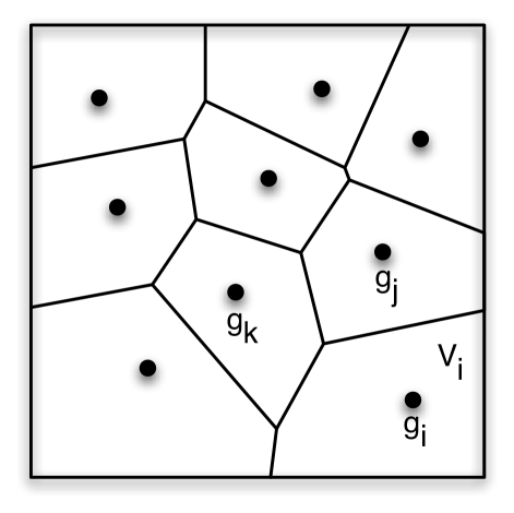
(a) A Voronoi Diagram.

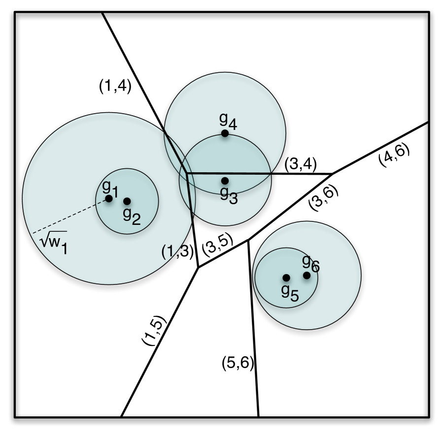
(b) A power diagram. The weights $w_{i}$ are assumed positive. Circles represent the magnitudes of weights. Power generator $(g_{2},w_{2})$ has an empty cell. Power generator $(g_{5},w_{5})$ is outside its region of dominance.

Figure 1: Voronoi diagrams and power diagrams.

II-E Proximity Graphs and Spatially-Distributed Control Policies for Robotic Networks

Next, we shall present some relevant concepts on proximity graph functions and spatially-distributed control policies; we refer the reader to [15] for a more detailed discussion. A proximity graph function $\mathcal{G}:\mathbb{F}({\mathbb{R}}^{d})\to\mathbb{G}({\mathbb{R}}^{d})$ associates to a point set $\mathcal{P}\in\mathbb{F}({\mathbb{R}}^{d})$ an undirected graph with vertex set $\mathcal{P}$ and edge set $\mathcal{E}_{\mathcal{G}}(\mathcal{P})$, where $\mathcal{E}_{\mathcal{G}}:\mathbb{F}({\mathbb{R}}^{d})\mapsto\mathbb{F}({\mathbb{R}}^{d}\times{\mathbb{R}}^{d})$ has the property that $\mathcal{E}_{\mathcal{G}}(\mathcal{P})\subset\mathcal{P}\times\mathcal{P}\setminus\text{diag}(\mathcal{P}\times\mathcal{P})$ for any $\mathcal{P}$ . Here, $\text{diag}(\mathcal{P}\times\mathcal{P})=\{(p,p)\in\mathcal{P}\times\mathcal{P}|\,\,p\in\mathcal{P}\}$. In other words, the edge set of a proximity graph depends on the location of its vertices. To each proximity graph function, one can associate the set of neighbors map $N_{\mathcal{G}}:{\mathbb{R}}^{d}\times\mathbb{F}({\mathbb{R}}^{d})\to\mathbb{F}({\mathbb{R}}^{d})$, defined by

$$N_{\mathcal{G}}(p,\mathcal{P})=\{q\in\mathcal{P}|\,\,(p,q)\in\mathcal{E}_{\mathcal{G}}(\mathcal{P}\cup\{p\})\}.$$

Two examples of proximity graph functions are:

1. the Delaunay graph $G\mapsto\mathcal{G}_{\text{V}}(G)=(G,\mathcal{E}_{\mathcal{G}_{\text{V}}}(G))$ has edge set

   $$\mathcal{E}_{\mathcal{G}_{\text{V}}}(G)=\{(g_{i},g_{j})\in G\times G\setminus\text{diag}(G\times G)|\,\,V_{i}(G)\cap V_{j}(G)\neq\emptyset\},$$

   where $V_{i}(G)$ is the $i$-th cell in the Voronoi diagram $\mathcal{V}(G)$;

2. the power-Delaunay graph $G_{W}\mapsto\mathcal{G}_{\text{P}}(G_{W})=(G_{W},\mathcal{E}_{\mathcal{G}_{\text{P}}}(G_{W}))$ has edge set

   $$\mathcal{E}_{\mathcal{G}_{\text{P}}}(G_{W})=\Bigl{\{}\Bigl{(}g_{i},w_{i}),(g_{j},w_{j})\Bigr{)}\in G_{W}\times G_{W}\setminus\text{diag}(G_{W}\times G_{W})|\,\,V_{i}(G_{W})\cap V_{j}(G_{W})\neq\emptyset\Bigr{\}},$$

   where $V_{i}(G_{W})$ is the $i$-th cell in the power diagram $\mathcal{V}(G_{W})$.

We are now in a position to discuss spatially-distributed algorithms for robotic networks in formal terms. Let $P(t)=(p_{1}(t),\ldots,p_{m}(t))\in A^{m}$ be the ordered set of positions of $m$ agents in a robotic network. We denote the state of each agent $i\in I_{m}$ at time $t$ as $x_{i}(t)\in{\mathbb{R}}^{q}$ ($x_{i}(t)$ can include the position of agent $i$ as well as other information). With a slight abuse of notation, let us denote by $I_{i}(t)$ the information available to agent $i$ at time $t$. The information vector $I_{i}(t)$ is a subset of $x(t)\doteq(x_{1}(t),\ldots,x_{m}(t))$ of the form $I_{i}(t)=\{x_{i_{1}}(t),\ldots,x_{i_{k}}(t)\}$, $k\leq m$. We assume that $I_{i}(t)$ always includes $x_{i}(t)$. Let $\mathcal{G}$ be a proximity graph function defined over $P(t)$ (respectively over $P_{W}(t)$ if we also consider a weight $w_{i}(t)$ for each robot $i\in I_{m}$); we define $I_{i}^{N_{\mathcal{G}}}(t)$ as the information vector with the property $x_{i}(t)\in I_{i}^{N_{\mathcal{G}}}(t)$, and, for $j\neq i$,

$$x_{j}(t)\in I_{i}^{N_{\mathcal{G}}}(t)\Leftrightarrow p_{j}(t)\in N_{\mathcal{G}}(p_{i}(t),P(t))\quad\biggl{(}\,\Leftrightarrow(p_{j}(t),w_{j}(t))\in N_{\mathcal{G}}\Bigl{(}(p_{i}(t),w_{i}(t)),P_{W}(t)\Bigr{)},\,\,\text{respectively}\biggr{)}.$$

In words, the information vector $I_{i}^{N_{\mathcal{G}}}(t)$ coincides with the states of the neighbors (as induced by $\mathcal{G}$) of agent $i$ together with the state of agent $i$ itself.

Let $\mu(t)=(\mu_{1}(I_{1}(t)),\ldots,\mu_{m}(I_{m}(t))$ be a feedback control policy for the robotic network. The policy $\mu$ is spatially distributed over $\mathcal{G}$ if for each agent $i\in I_{m}$ and for all $t$

$$\mu_{i}(I_{i}(t))=\mu_{i}\Bigl{(}I_{i}^{N_{\mathcal{G}}}(t)\Bigr{)}.$$

In other words, through information about its neighbors according to $\mathcal{G}$, each agent $i$ has sufficient information to compute the control $\mu_{i}$.

III Problem Formulation

A total of $m$ identical mobile agents provide service in a compact, convex service region $A\subseteq{\mathbb{R}}^{d}$. Let $\lambda$ be a measure whose bounded support is $A$ (in other words, $\lambda$ is not zero only on $A$); for any set $S$, we define the workload for region $S$ as $\lambda_{S}\doteq\int_{S}\lambda(x)\,dx$. The measure $\lambda$ models service requests, and can represent, for example, the density of customers over $A$, or, in a stochastic setting, their arrival rate. Given the measure $\lambda$, a partition $\{A_{i}\}_{i}$ of the workspace $A$ is equitable if $\lambda_{A_{i}}=\lambda_{A_{j}}$ for all $i,\,j\in I_{m}$.

A partitioning policy is an algorithm that, as a function of the number $m$ of agents and, possibly, of their position and other information, partitions a bounded workspace $A$ into $m$ openly disjoint subregions $A_{i}$, $i\in I_{m}$. Then, each agent $i$ is assigned to subregion $A_{i}$, and each service request in $A_{i}$ receives service from the agent assigned to $A_{i}$. We refer to subregion $A_{i}$ as the region of dominance of agent $i$. Given a measure $\lambda$ and a partitioning policy, $m$ agents are in a convex equipartition configuration with respect to $\lambda$ if the associated partition is equitable and convex.

In this paper we study the following problem: find a spatially-distributed (in the sense discussed in Section II) equitable partitioning policy that allows $m$ mobile agents to achieve a convex equipartition configuration (with respect to $\lambda$). Moreover, we consider the issue of convergence to equitable partitions with some special properties, e.g., where subregions have shapes similar to those of regular polygons.

IV Leader-Election Policies

We first describe two simple algorithms that provide equitable partitions. A first possibility is to “sweep” $A$ from a point in the interior of $A$ using an arbitrary starting ray until $\lambda_{A_{1}}=\lambda_{A}/m$, continuing the sweep until $\lambda_{A_{2}}=\lambda_{A}/m$, etc. A second possibility is to slice, in a similar fashion, $A$. The resulting equitable partitions are depicted in Fig. 2

    

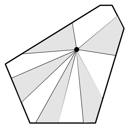
(a) Sweeping $A$

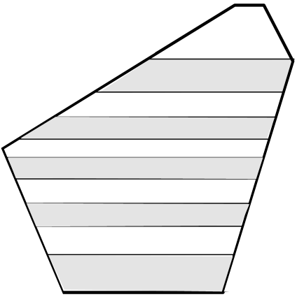
(b) Slicing $A$

Figure 2: Equitable partitions by sweeping and slicing (assuming a uniform measure $\lambda$).

Then, a possible solution could be to (i) run a distributed leader election algorithm over the graph associated to some proximity graph function $\mathcal{G}$ (e.g., the Delaunay graph); (ii) let each agent send its state $x_{i}(t)$ to the leader; (iii) let the leader execute either the sweeping or the slicing algorithms described above; finally, (iv), let the leader broadcast subregion’s assignments to all other agents. Such conceptually simple solution, however, can be impractical in scenarios where the density $\lambda$ changes over time, or agents can fail, since at every parameter’s change a new time-consuming leader election is needed. Moreover, the sweeping and the slicing algorithms provide long and skinny subregions that are not suitable in most applications of interest (e.g., vehicle routing).

We now present spatially-distributed algorithms, based on the concept of power diagrams, that solve both issues at once.

V Spatially-Distributed Gradient-Descent Law for Equitable Partitioning

We start this section with an existence theorem for equitable power diagrams.

V-A On the Existence of Equitable Power Diagrams

As shown in the next theorem, an equitable power diagram (with respect to any $\lambda$) exists for any vector of distinct points $G=(g_{1},\ldots,g_{n})$ in $A$.

Theorem V.1

Let $A$ be a bounded, connected domain in ${\mathbb{R}}^{d}$, and $\lambda$ be a measure on $A$. Let $G=(g_{1},\dots,g_{n})$ be the positions of $n\geq 1$ distinct points in $A$. Then, there exist weights $w_{i}$, $i\in I_{n}$, such that the power points $\Bigl{(}(g_{1},w_{1}),\ldots,(g_{n},w_{n})\Bigr{)}$ generate a power diagram that is equitable with respect to $\lambda$. Moreover, given a vector of weights $w^{*}$ that yields an equitable power diagram, the set of all vectors of weights yielding an equitable power diagram is $\mathcal{W}^{*}_{t}\doteq\{w^{*}+t[1,\ldots,1]\}$, with $t\in{\mathbb{R}}$.

Proof:

It is not restrictive to assume that $\lambda_{A}=1$ (i.e., we normalize the measure of $A$), since $A$ is bounded. The strategy of the proof is to use a topological argument to force existence.

First, we construct a weight space. Let $D=\mathrm{diameter}(A)$, and consider the cube $\mathcal{C}:=[-D,D]^{n}$. This is the weight space and we consider weight vectors $W$ taking value in $\mathcal{C}$. Second, consider the standard $n$-simplex of measures $\lambda_{A_{1}},\ldots,\lambda_{A_{n}}$ (where $A_{1},\dots,A_{n}$ are, as usual, the regions of dominance). This can be realized in $\mathbb{R}^{n}$ as the subset of defined by $\sum_{i=1}^{n}\lambda_{A_{i}}=1$ with the condition $\lambda_{A_{i}}\geq 0$. Let us call this set “the measure simplex $\mathcal{A}$” (notice that it is $(n-1)$-dimensional).

There is a map $f:\mathcal{C}\rightarrow\mathcal{A}$ associating, according to the power distance, a weight vector $W$ with the corresponding vector of measures $(\lambda_{A_{1}},\ldots,\lambda_{A_{n}})$. Since the points in $G$ are assumed to be distinct, this map is continuous.

We will now use induction on $n$, starting with the base case $n=3$ (the statement for $n=1$ and $n=2$ is trivially checked). We study in detail the case for $n=3$, where visualization is easier, in order to make the proof more transparent. When $n=3$, the weight space $\mathcal{C}$ is a three dimensional cube with vertices $v_{0}=[-D,-D,-D],$ $v_{1}=[D,-D,-D],$ $v_{2}=[-D,D,-D],$ $v_{3}=[-D,-D,D],$ $v_{4}=[D,-D,D],$ $v_{5}=[-D,D,D],$ $v_{6}=[D,D,-D]$ and $v_{7}=[D,D,D]$. The measure simplex $\mathcal{A}$ is, instead, a triangle with vertices $u_{1},u_{2},u_{3}$ that correspond to the cases $\lambda_{A_{1}}=1,\lambda_{A_{2}}=0,\lambda_{A_{3}}=0$, $\lambda_{A_{1}}=0,\lambda_{A_{2}}=1,\lambda_{A_{3}}=0$, and $\lambda_{A_{1}}=0,\lambda_{A_{2}}=0,\lambda_{A_{3}}=1$, respectively. Moreover, call $e_{1},e_{2}$ and $e_{3}$ the edges opposite the vertices $u_{1},u_{2},u_{3}$ respectively. The edges $e_{i}$ are, therefore, given by the condition $\lambda_{A_{i}}\in e_{i}\Leftrightarrow\lambda_{A_{i}}=0$.

Let us return to the map $f:\mathcal{C}\rightarrow\mathcal{A}$ (now in the case of three generators). Observe that the map $f$ sends $v_{0}$ the unique point $p_{0}$ of $\mathcal{A}$ corresponding to the measures of usual Voronoi cells (since the weights are all equal). Call $l_{1}$ the edge $v_{0}v_{1}$; then, it is immediate to see that the image of $l_{1}$ through $f$ is a path $\gamma_{1}$ in $\mathcal{A}$ joining $p_{0}$ to $u_{1}$. Analogously, the image of $l_{2}=v_{0}v_{2}$ through $f$ is a path $\gamma_{2}$ in $\mathcal{A}$ joining $p_{0}$ to $u_{2}$ and, finally, the image of $l_{3}=v_{0}v_{3}$ through $f$ is a path $\gamma_{3}$ connecting $p_{0}$ to $u_{3}$ (see Fig. 3). Now, we observe that paths $\{\gamma_{i}\}_{\{i=1,2,3\}}$ do not intersect except in $p_{0}$. To prove this, start by observing that the image through $f$ of all the points on the main diagonal of the cube joining $v_{0}$ with $v_{7}$ is equal to a single point $p_{0}\in\mathcal{A}$. This is due to the fact that only the differences among weights change the vector $(\lambda_{A_{1}},\lambda_{A_{2}},\lambda_{A_{3}})$, i.e., if all weights are increased by the same quantity, the vector $(\lambda_{A_{1}},\lambda_{A_{2}},\lambda_{A_{3}})$ does not change. We will prove this in detail for the case of $n$-generators in the next few paragraphs. In particular, the image of the diagonal $v_{0}v_{7}$ is exactly the point for which the measures are those of a Voronoi partition. Now let us understand what are the “fibers” of $f$, that is to say, the loci where $f$ is constant. Since the measures of the regions of dominance do not change if the differences among the weights are kept constant, then the fibers of $f$ in the weight space $\mathcal{C}$ are given by the equations $w_{1}-w_{2}=c_{1}$ and $w_{2}-w_{3}=c_{2}$. Rearranging these equations, it is immediate to see that $w_{1}=w_{3}+c_{1}+c_{2}$, $w_{2}=w_{3}+c_{2}$ and $w_{3}=w_{3}$, therefore taking $w_{3}$ as parameter we see that the fibers of $f$ are straight lines parallel to the main diagonal $v_{0}v_{7}$. On the weight space $\mathcal{C}$ let us define the following equivalence relation: $w\equiv w^{\prime}$ if and only if they are on a line parallel to the main diagonal $v_{0}v_{7}$. Map $f:\mathcal{C}\rightarrow\mathcal{A}$ induces a continuous map (still called $f$ by abuse of notation) from $\mathcal{C}/\equiv$ to $\mathcal{A}$ having the same image. Let us identify $\mathcal{C}/\equiv$. It is easy to see that any line in the cube parallel to the main diagonal $v_{0}v_{7}$ is entirely determined by its intersection with the three faces $F_{3}=\{w_{3}=-D\}\cap\mathcal{C}$, $F_{2}=\{w_{2}=-D\}\cap\mathcal{C}$ and $F_{1}=\{w_{1}=-D\}\cap\mathcal{C}$. Call $\mathcal{F}$ the union of these faces. We therefore have a continuous map $f:\mathcal{F}\rightarrow\mathcal{A}$ that has the same image of original $f$; besides, in the few next paragraphs we will prove in general (i.e for the case with $n$ generators) that the induced map $f:\mathcal{F}\rightarrow\mathcal{A}$ is injective by construction.

Observe that $\mathcal{F}$ is homeomorphic to $B^{2}$, the $2$-dimensional ball, like $\mathcal{A}$ itself. Up to homeomorphisms, therefore, the map $f:\mathcal{F}\rightarrow\mathcal{A}$ can be viewed as a map (again called $f$ by abuse of notation), $f:B^{2}\rightarrow B^{2}$. Consider the closed loop $\alpha$ given by $v_{2}v_{5}$, $v_{5}v_{3}$, $v_{3}v_{4}$, $v_{4}v_{1}$, $v_{1}v_{6}$, $v_{6}v_{2}$ with this orientation. This loop is the boundary of $\mathcal{F}$ and we think of it also as the boundary of $B^{2}$. It is easy to see that $f$ maps $\alpha$ onto the boundary of $A$, and since $f$ is injective, the inverse image of any point in the boundary of $A$ is just one element of $\alpha$. Identifying the boundary of $\mathcal{A}$ with $S^{1}$ (up to homeomorphisms) and the loop $\alpha$ with $S^{1}$ (up to homeomorphisms) we have a bijective continuous map $f_{S^{1}}:S^{1}\rightarrow S^{1}$. By Lemma (II.2) $\mathrm{deg}(f)=\pm 1$ and therefore $f$ is onto $\mathcal{A}$, using Theorem (II.1).

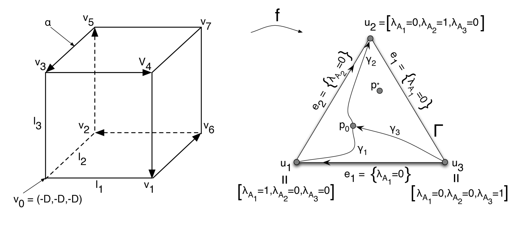
Figure 3: Construction used for the proof of existence of equitable power diagrams.

Now we extend the same idea to the case of $n$ generators and we will use also induction on the number of agents. Therefore, we suppose that we have proved that the map $f$ is surjective for $n-1$ agents and we show how to use this to show that the map is surjective for $n$ agents.

If we have $n$ generators, the weight space is given by an $n$ dimensional cube $\mathcal{C}=[-D,D]^{n}$, in complete analogy with the case of $3$ generators. The $n$ simplex of the areas $\mathcal{A}$ is again defined as a $\{(\lambda_{A_{1}},\dots,\lambda_{A_{n}})\in\mathbb{R}^{n}\}$ such that $\lambda_{A_{i}}\geq 0$ for $i=1,\dots,n$ and $\sum_{i=1}^{n}\lambda_{A_{i}}=1$. Notice that $\mathcal{A}$ is homeomorphic to the $(n-1)$-dimensional ball $B^{n-1}$. As before we have a continuous map $f:\mathcal{C}\rightarrow\mathcal{A}$. It is easy to see that $f$ is constant on the sets of the form $W^{*}_{t}:=\{\{w^{*}+t(1,\dots,1)\}\cap\mathcal{C},\quad t\in\mathbb{R}\}$, that is whenever two sets of weights differ by a common quantity, they are mapped to the same point in $\mathcal{A}$. Moreover, fixing a point $Q\in\mathcal{A}$ we have that $f^{-1}(Q)$ is given just by a set of the form $W^{*}_{t}$ for a suitable $w^{*}$. Indeed, assume this is not the case, then the vector of measures $(\lambda_{A_{1}},\dots,\lambda_{A_{n}})$ is obtained via $f$ using two sets of weights: $\mathcal{W}^{1}:=(w_{1}^{1},\dots w_{n}^{1})$ and $\mathcal{W}^{2}:=(w_{1}^{2},\dots w_{n}^{2})$, and $\mathcal{W}^{1}$ and $\mathcal{W}^{2}$ don’t belong to the same $W^{*}_{t}$, namely it is is not possible to obtain $\mathcal{W}^{2}$ as $\mathcal{W}^{1}+t(1,\dots,1)$ for a suitable $t$. This means that the vector difference $\mathcal{W}^{2}-\mathcal{W}^{1}$ is not a multiple of $(1,\dots,1)$. Therefore, there exists a nonempty set of indexes $J$, such that $w^{2}_{j}-w^{1}_{j}\geq w^{2}_{k}-w^{1}_{k}$, whenever $j\in J$ and for all $k\in\{1,\dots n\}$ and such that the previous inequality is strict for at least one $k^{*}$. Now among the indexes in $J$, there exists at least one of them, call it $j^{*}$ such that the agent $j^{*}$ is a neighbor of agent $k^{*}$, due to the fact that the domain $A$ is connected. But since $w^{2}_{j^{*}}-w^{1}_{j^{*}}>w^{2}_{k^{*}}-w^{1}_{k^{*}}$, and $w^{2}_{j^{*}}-w^{1}_{j^{*}}\geq w^{2}_{k}-w^{1}_{k}$ for all $k\in\{1,\dots,n\}$, this implies that the measure $\lambda_{A_{j^{*}}}$ corresponding to the choice of weights $\mathcal{W}^{2}$ is strictly greater that $\lambda_{A_{j^{*}}}$ corresponding to the choice of weights $\mathcal{W}^{1}$. This proves that $f^{-1}(Q)$ is given only by sets of the form $W^{*}_{t}$.

We introduce an equivalence relation on $\mathcal{C}$, declaring that two sets of weights $\mathcal{W}^{1}$ and $\mathcal{W}^{2}$ are equivalent if and only if they belong to the same $W^{*}_{t}$. Let us call $\equiv$ this equivalence relation. It is immediate to see that $f$ descends to a map, still called $f$ by abuse of notation, $f:\mathcal{C}/\equiv\rightarrow\mathcal{A}$ and that $f$ is now injective. It is easy also to identify $\mathcal{C}/\equiv$ with the union of the $(n-1)$-dimensional faces of $\mathcal{C}$ given by $\mathcal{F}=\cup_{i=1}^{n}(\mathcal{C}\cap\{w_{i}=-D\})$. In this way we get a continuous injective map $f:\mathcal{F}\rightarrow\mathcal{A}$ that has the same image as the original $f$. Notice also that $\mathcal{F}$ is homeomorphic to the closed $(n-1)$-dimensional ball, so up to homeomorphism $f$ can be viewed as a map $f:B^{n-1}\rightarrow B^{n-1}$.

We want to prove that the map $f_{\partial\mathcal{F}}$, given by the restriction of $f$ to $\partial\mathcal{F}$ is onto $\partial\mathcal{A}$. To see this, consider one of the $(n-2)$-dimensional faces $\partial\mathcal{A}_{i}$ of $\partial\mathcal{A}$, which is identified by the condition $\lambda_{A_{i}}=0$. Consider the face $F_{i}$ in $\mathcal{F}$, where $F_{i}$ is given by $F_{i}:=\mathcal{C}\cap\{w_{i}=-D\}$. We claim that the $S_{i}:=\partial F_{i}\cap\partial\mathcal{F}$ is mapped onto $\partial\mathcal{A}_{i}$ by $f$. Observe that the $S_{i}$ is described by the following equations $S_{i}=\cup_{j\neq i}(\{w_{i}=-D,w_{j}=D\}\cap\mathcal{F})$, so $S_{i}$ is exactly equivalent to a set of type $\mathcal{F}$ for $n-1$ agents. Moreover observe that $\partial\mathcal{A}_{i}$ can also be identified with the measure simplex for $n-1$ agents. By inductive hypothesis therefore, the map $f:S_{i}\rightarrow\partial\mathcal{A}_{i}$ is surjective, and therefore also the map $f_{\partial\mathcal{F}}$ is onto $\partial\mathcal{A}$. Since $f_{\partial\mathcal{F}}$ is a bijective continuos map among $(n-2)$-dimensional spheres, (up to homeomorphism), it has degree $\pm 1$ by Lemma (II.2). Finally we conclude that $f$ is onto $\mathcal{A}$, using again Theorem (II.1).

∎

Some remarks are in order.

Remark V.2

The above theorem holds for any bounded, connected domain in ${\mathbb{R}}^{d}$. Thus, the case of a compact, convex subset of ${\mathbb{R}}^{d}$ is included as a special case. Moreover, it holds for any measure $\lambda$ absolutely continuous with respect to the Lebesgue measure, and for any vector of distinct points in $A$.

Remark V.3

In the proof of the above theorem, we actually proved that for any measure vector $\{\lambda_{A_{i}}\}_{i=1,\dots m}$ in $\mathcal{A}$, there exists a weight vector $w\in C$ realizing it through the map $f$. This could be useful in some applications.

Remark V.4

Since all vectors of weights in $\mathcal{W}$ yield exactly the same power diagram, we conclude that the positions of the generators uniquely induces an equitable power diagram.

V-B State, Region of Dominance, and Locational Optimization

The first step is to define the state for each agent $i$. We let $x_{i}(t)$ be the power generator $(g_{i}(t),w_{i}(t))\in A\times{\mathbb{R}}$, where $g_{i}(t)=p_{i}(t)$ (i.e., the position of the power generator coincides with the position of the agent) . We, then, define the region of dominance for agent $i$ as the power cell $V_{i}=V_{i}(G_{W})$, where $G_{W}=\Bigl{(}(g_{1},w_{1}),\cdots,(g_{m},w_{m})\Bigr{)}$. We refer to the partition into regions of dominance induced by the set of generators $G_{W}$ as $\mathcal{V}(G_{W})$.

In light of Theorem V.1, the key idea is to enable the weights of the generators to follow a spatially-distributed gradient descent law (while maintaining the positions of the generators fixed) such that an equitable partition is reached. Assume, henceforth, that the positions of the generators are distinct, i.e., $g_{i}\neq g_{j}$ for $i\neq j$. Define the set

$$S\doteq\Bigl{\{}(w_{1},\ldots,w_{m})\in{\mathbb{R}}^{m}\,|\,\lambda_{V_{i}}>0\,\,\,\forall i\in I_{m}\Bigr{\}}.$$ (9)

Set $S$ contains all possible vectors of weights such that no region of dominance has measure equal to zero.

We introduce the locational optimization function $H_{V}:S\mapsto{\mathbb{R}}_{>0}$:

$$H_{V}(W)\doteq\sum_{i=1}^{m}\Bigl{(}\int_{V_{i}(W)}\!\lambda(x)dx\Bigr{)}^{-1}=\sum_{i=1}^{m}\lambda_{V_{i}(W)}^{-1}.$$ (10)

where $W\doteq(w_{1},\cdots,w_{m})$.

Lemma V.5

A vector of weights that yields an equitable power diagram is a global minimum of $H_{V}$.

Proof:

Consider the relaxation of our minimization problem:

$$\min_{x_{1},\cdots,x_{m}}\sum_{i=1}^{m}x_{i}^{-1}\,;\quad\text{s.t. }\sum_{i=1}^{m}x_{i}=a>0,\quad x_{i}>0,\;i\in I_{m},$$

where the linear equality constraint follows from the fact that $\sum_{i=1}^{m}\int_{V_{i}(W)}\lambda(x)dx$ $=\int_{A}\lambda(x)\,dx\doteq a$ and where the constant $a$ is greater than zero since $\lambda$ is a measure whose bounded support is $A$. By Lagrange multiplier arguments, it is immediate to show that the global minimum for the relaxation is $x_{i}=a/m$ for all $i$. Since Theorem V.1 establishes that there exists a vector of weights in $S$ that yields an equitable power diagram, we conclude that this vector is a global minimum of $H_{V}$. ∎

V-C Smoothness and Gradient of $H_{V}$

We now analyze the smoothness properties of $H_{V}$. In the following, let $\gamma_{ij}\doteq\|g_{j}-g_{i}\|$.

Theorem V.6

Assume that the positions of the generators are distinct, i.e., $g_{i}\neq g_{j}$ for $i\neq j$. Given a measure $\lambda$, the function $H_{V}$ is continuously differentiable on $S$, where for each $i\in\{1,\dots,m\}$

$$\begin{split}\frac{\partial H_{V}}{\partial\,w_{i}}&=\sum_{j\in N_{i}}\frac{1}{2\gamma_{ij}}\Bigl{(}\frac{1}{\lambda_{V_{j}}^{2}}-\frac{1}{\lambda_{V_{i}}^{2}}\Bigr{)}\int_{\Delta_{ij}}\lambda(x)\,dx.\end{split}$$ (11)

Furthermore, the critical points of $H_{V}$ are vectors of weights that yield an equitable power diagram.

Proof:

By assumption, $g_{i}\neq g_{j}$ for $i\neq j$, thus the power diagram is well defined. Since the motion of a weight $w_{i}$ affects only power cell $V_{i}$ and its neighboring cells $V_{j}$ for $j\in N_{i}$, we have

$$\frac{\partial H_{V}}{\partial w_{i}}=-\frac{1}{\lambda_{V_{i}}^{2}}\frac{\partial\lambda_{V_{i}}}{\partial w_{i}}-\sum_{j\in N_{i}}\frac{1}{\lambda_{V_{j}}^{2}}\frac{\partial\lambda_{V_{j}}}{\partial w_{i}}.$$ (12)

Now, the result in Eq. (2) provides the means to analyze the variation of an integral function due to a domain change. Since the boundary of $V_{i}$ satisfies $\partial V_{i}=\cup_{j}\Delta_{ij}\cup B_{i}$, where $\Delta_{ij}=\Delta_{ji}$ is the edge between $V_{i}$ and $V_{j}$, and $B_{i}$ is the boundary between $V_{i}$ and $A$ (if any, otherwise $B_{i}=\emptyset$), we have

$$\begin{split}\frac{\partial\lambda_{V_{i}}}{\partial w_{i}}=\sum_{j\in N_{i}}&\int_{\Delta_{ij}}\Bigl{(}\frac{\partial x}{\partial w_{i}}\cdot n_{ij}(x)\Bigr{)}\,\lambda(x)\,dx+\underbrace{\int_{B_{i}}\Bigl{(}\frac{\partial x}{\partial w_{i}}\cdot n_{ij}(x)\Bigr{)}\,\lambda(x)\,dx}_{=0},\end{split}$$ (13)

where we defined $n_{ij}$ as the unit normal to $\Delta_{ij}$ outward of $V_{i}$ (therefore we have $n_{ji}=-n_{ij}$). The second term is trivially equal to zero if $B_{i}=\emptyset$; it is also equal to zero if $B_{i}\neq\emptyset$, since the integrand is zero almost everywhere. Similarly,

$$\begin{split}\frac{\partial\lambda_{V_{j}}}{\partial w_{i}}=&\int_{\Delta_{ij}}\Bigl{(}\frac{\partial x}{\partial w_{i}}\cdot n_{ji}(x)\Bigr{)}\,\lambda(x)\,dx.\end{split}$$ (14)

To evaluate the scalar product between the boundary points and the unit outward normal to the border in Eq. (13) and in Eq. (14), we differentiate Eq. (7) with respect to $w_{i}$ at every point $x\in\Delta_{ij}$; we get

$$\frac{\partial x}{\partial w_{i}}\cdot(g_{j}-g_{i})=\frac{1}{2}.$$ (15)

From Eq. (7) we have $n_{ij}=~{}(g_{j}-~{}g_{i})~{}/\|g_{j}-g_{i}\|$, and the desired explicit expressions for the scalar products in Eq. (13) and in Eq. (14) follow immediately (recalling that $n_{ji}=-n_{ij}$).

Collecting the above results, we get the partial derivative with respect to $w_{i}$. The proof of the characterization of the critical points is an immediate consequence of the expression for the gradient of $H_{V}$; we omit it in the interest of brevity. ∎

Remark V.7

The computation of the gradient in Theorem V.6 is spatially-distributed over the power-Delaunay graph, since it depends only on the location of the other agents with contiguous power cells.

Example V.8 (Gradient of $H_{V}$ for uniform measure)

The gradient of $H_{V}$ simplifies considerably when $\lambda$ is constant. In such case, it is straightforward to verify that (assuming that $\lambda$ is normalized)

$$\begin{split}\frac{\partial H_{V}}{\partial\,w_{i}}&=\frac{1}{2|A|}\sum_{j\in N_{i}}\frac{\delta_{ij}}{\gamma_{ij}}\Bigl{(}\frac{1}{|V_{j}|^{2}}-\frac{1}{|V_{i}|^{2}}\Bigr{)},\end{split}$$ (16)

where $\delta_{ij}$ is the length of the border $\Delta_{ij}$.

V-D Spatially-Distributed Algorithm for Equitable Partitioning

Consider the set $U\doteq\Bigl{\{}(w_{1},\ldots,w_{m})\in{\mathbb{R}}^{m}\,|\,\sum_{i=1}^{m}w_{i}=0\Bigr{\}}$. Since adding an identical value to every weight leaves all power cells unchanged, there is no loss of generality in restricting the weights to $U$; let $\Omega\doteq S\cap U$. Assume the generators’ weights obey a first order dynamical behavior described by

$$\dot{w}_{i}=u_{i}.$$

Consider $H_{V}$ an objective function to be minimized and impose that the weight $w_{i}$ follows the gradient descent given by (11). In more precise terms, we set up the following control law defined over the set $\Omega$

$$u_{i}=-\frac{\partial H_{V}}{\partial w_{i}}(W),$$ (17)

where we assume that the partition $\mathcal{V}(W)=\{V_{1},\ldots,V_{m}\}$ is continuously updated. One can prove the following result.

Theorem V.9

Assume that the positions of the generators are distinct, i.e. $g_{i}\neq g_{j}$ for $i\neq j$. Consider the gradient vector field on $\Omega$ defined by equation (17). Then generators’ weights starting at $t=0$ at $W(0)\in\Omega$, and evolving under (17) remain in $\Omega$ and converge asymptotically to a critical point of $H_{V}$, i.e., to a vector of weights yielding an equitable power diagram.

Proof:

We first prove that generators’ weights evolving under (17) remain in $\Omega$ and converge asymptotically to the set of critical points of $H_{V}$. By assumption, $g_{i}\neq g_{j}$ for $i\neq j$, thus the power diagram is well defined. First, we prove that set $\Omega$ is positively invariant with respect to (17). Recall that $\Omega=S\cap U$. Noticing that control law (17) is a gradient descent law, we have

$$\lambda_{V_{i}(W(t))}^{-1}\leq H_{V}(W(t))\leq H_{V}(W(0)),\quad i\in I_{m},\,\,t\geq 0.$$

Since the measures of the power cells depend continuously on the weights, we conclude that the measures of all power cells will be bounded away from zero; thus, the weights will belong to $S$ for all $t\geq 0$, that is, $W(t)\in S$ $\forall t\geq 0$. Moreover, the sum of the weights is invariant under control law (17). Indeed,

$$\frac{\partial\sum_{i=1}^{m}w_{i}}{\partial t}=-\sum_{i=1}^{m}\frac{\partial H_{V}}{\partial w_{i}}=-\sum_{i=1}^{m}\sum_{j\in N_{i}}\frac{1}{2\gamma_{ij}}\Bigl{(}\frac{1}{\lambda_{V_{j}}^{2}}-\frac{1}{\lambda_{V_{i}}^{2}}\Bigr{)}\int_{\Delta_{ij}}\lambda(x)\,dx=0,$$

since $\gamma_{ij}=\gamma_{ji}$, $\Delta_{ij}=\Delta_{ji}$, and $j\in N_{i}\Leftrightarrow i\in N_{j}$. Thus, we have $W(t)\in U$ $\forall t\geq 0$. Since $W(t)\in S$ $\forall t\geq 0$ and $W(t)\in U$ $\forall t\geq 0$, we conclude that $W(t)\in S\cap U=\Omega$, $\forall t\geq 0$, that is, set $\Omega$ is positively invariant.

Second, $H_{V}:\Omega\to{\mathbb{R}}_{\geq 0}$ is clearly non-increasing along system trajectories, that is, $\dot{H}_{V}\leq 0$ in $\Omega$.

Third, all trajectories with initial conditions in $\Omega$ are bounded. Indeed, we have already shown that $\sum_{i=1}^{m}w_{i}=0$ along system trajectories. This implies that weights remain within a bounded set: If, by contradiction, a weight could become arbitrarily positive large, another weight would become arbitrarily negative large (since the sum of weights is constant), and the measure of at least one power cell would vanish, which contradicts the fact that $S$ is positively invariant.

Finally, by Theorem V.6, $H_{V}$ is continuously differentiable in $\Omega$. Hence, by invoking the LaSalle invariance principle (see, for instance, [6]), under the descent flow (17), weights will converge asymptotically to the set of critical points of $H_{V}$, that is not empty as confirmed by Theorem V.1.

Indeed, by Theorem V.1, we know that all vectors of weights yielding an equitable power diagram differ by a common translation. Thus, the largest invariant set of $H_{V}$ in $\Omega$ contains only one point. This implies that $\lim_{t\to\infty}W(t)$ exists and it is equal to a vector of weights that yields an equitable power diagram.

∎

Some remarks are in order.

Remark V.10

By Theorem V.9, for any set of generators’ distinct positions, convergence to an equitable power diagram is global with respect to $\Omega$. Indeed, there is a very natural choice for the initial values of the weights. Assuming that at $t=0$ agents are in $A$ and in distinct positions, each agent initializes its weight to zero. Then, the initial partition is a Voronoi tessellation; since $\lambda$ is positive on $A$, each initial cell has nonzero measure, and therefore $W(0)\in\Omega$ (the sum of the initial weights is clearly zero).

Remark V.11

The partial derivative of $H_{V}$ with respect to the $i$-th weight only depends on the weights of the agents with neighboring power cells. Therefore, the gradient descent law (17) is indeed a spatially-distributed control law over the power-Delaunay graph. We mention that, in a power diagram, each power generator has an average number of neighbors less than or equal to six [14]; therefore, the computation of gradient (17) is scalable with the number of agents.

Remark V.12

The focus of this paper is on equitable partitions. Notice, however, that it is easy to extend the previous algorithm to obtain a spatially-distributed (again over the power-Delaunay graph) control law that provides any desired measure vector $\{\lambda_{A_{i}}\}$. In particular, assume that we desire a partition such that

$$\lambda_{A_{i}}=\beta_{i}\lambda_{A},$$

where $\beta_{i}\in(0,\,1)$, $\sum_{j=1}^{m}\beta_{j}=1$. If we redefine $H_{V}:S\mapsto{\mathbb{R}}_{>0}$ as

$$H_{V}(W)\doteq\sum_{i=1}^{m}\frac{\beta_{i}^{2}}{\lambda_{V_{i}(W)}},$$

then, following the same steps as before, it is possible to show that, under control law

$$\dot{w}_{i}=-\frac{\partial H_{V}}{\partial w_{i}}(W)=\sum_{j\in N_{i}}\frac{1}{2\gamma_{ij}}\biggl{(}\frac{\beta^{2}_{j}}{\lambda_{V_{j}}^{2}}-\frac{\beta^{2}_{i}}{\lambda_{V_{i}}^{2}}\biggr{)}\int_{\Delta_{ij}}\lambda(x)\,dx,$$

the solution converges to a vector of weights that yields a power diagram with the property $\lambda_{A_{i}}=\beta_{i}\lambda_{A}$ (whose existence is guaranteed by Remark V.3).

Remark V.13

Define the set $\Gamma\doteq A^{m}\setminus\Gamma_{\text{coinc}}$ (where $\Gamma_{\text{coinc}}$ is defined in Eq. (4)). It is of interest to define and characterize the vector-valued function $W^{*}:\Gamma\mapsto\Omega$ that associates to each non-degenerate vector of generators’ positions a set of weights such that the corresponding power diagram is equitable. Precisely, we define $W^{*}(G)$ as $W^{*}(G)\doteq\lim_{t\to\infty}W(t),$ where $W(t)=(w_{1}(t),\ldots,w_{m}(t))$ is the solution of the differential equation, with fixed vector of generators’ positions $G$,

$$\dot{w_{i}}(t)=-\frac{\partial H_{V}}{\partial w_{i}}(W(t)),\quad w_{i}(0)=0,\quad i\in I_{m}.$$

By Theorem V.9, $W^{*}(G)$ is a well-defined quantity (since the limit exists) and corresponds to an equitable power diagram. The next lemma characterizes $W^{*}(G)$.

Lemma V.14

The function $W^{*}$ is continuous on $\Gamma$.

Proof:

See Appendix. ∎

V-E On the Use of Power Diagrams

A natural question that arises is whether a similar result can be obtained by using Voronoi diagrams (of which power diagrams are a generalization). The answer is positive if we constrain $\lambda$ to be constant over $A$, but it is negative for general measures $\lambda$, as we briefly discuss next.

Indeed, when $\lambda$ is constant over $A$, an equitable Voronoi diagram always exists. We prove this result in a slightly more general set-up.

Definition V.15 (Unimodal Property)

Let $A\subset{\mathbb{R}}^{d}$ be a bounded, measurable set (not necessarily convex). We say that $A$ enjoys the Unimodal Property if there exists a unit vector $v\in{\mathbb{R}}^{d}$ such that the following holds. For each $s\in{\mathbb{R}}$, define the slice $A^{s}\doteq\{x\in A,\quad v\cdot x=s\},$ and call $\psi(s)\doteq m_{d-1}(A^{s})$ the $(d-1)$-dimensional Lebesgue measure of the slice. Then, the function $\psi$ is unimodal. In other words, $\psi$ attains its global maximum at a point $\bar{s}$, is increasing on $(-\infty,\bar{s}]$, and decreasing on $[\bar{s},\infty)$.

The Unimodal Property (notice that every compact, convex set enjoys such property) turns out to be a sufficient condition for the existence of equitable Voronoi diagrams for bounded measurable sets (with respect to constant $\lambda$).

Theorem V.16

If $A\subset{\mathbb{R}}^{d}$ is any bounded measurable set satisfying the Unimodal Property and $\lambda$ is constant on $A$, then for every $m\geq 1$ there exists an equitable Voronoi diagram with $m$ (Voronoi) generators.

Proof:

See Appendix. ∎

Then, an equitable Voronoi diagram can be achieved by using a gradient descent law conceptually similar to the one discussed previously (the details are presented in [16]). We emphasize that the existence result on equitable Voronoi diagrams seems to be new in the rich literature on Voronoi tessellations.

While an equitable Voronoi diagram always exists when $\lambda$ is constant over $A$, in general, for non-constant $\lambda$, an equitable Voronoi diagram fails to exist, as the following counterexample shows.

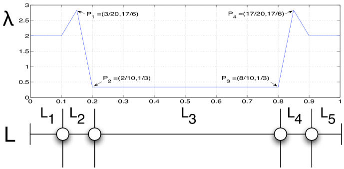
Figure 4: Example of non-existence of an equitable Voronoi diagram on a line. The above tessellation is an equitable partition, but not a Voronoi diagram.

Example V.17 (Existence problem on a line)

Consider a one-dimensional Voronoi diagram. In this case a Voronoi cell is a half line or a line segment (called a Voronoi line), and Voronoi vertices are end points of Voronoi lines. It is easy to notice that the boundary point between two adjacent Voronoi lines is the mid-point of the generators of those Voronoi lines. Consider the measure $\lambda$ in Fig. 4, whose support is the interval $[0,\,1]$. Assume $m=5$. Let $b_{i}$ ($i=1,\ldots,4$) be the position of the $i$-th rightmost boundary point and $g_{i}$ be the position of the $i$-th rightmost generator ($i=1,\ldots,5$). It is easy to verify that the only admissible configuration for the boundary points in order to obtain an equitable Voronoi diagram is the one depicted in Fig. 4. Now, by the Perpendicular Bisector Property, we require:

$$\left\{\begin{array}[]{l}g_{3}-b_{2}=b_{2}-g_{2}\\ g_{4}-b_{3}=b_{3}-g_{3}\end{array}\right.$$

Therefore, we would require $g_{4}-g_{2}=2(b_{3}-b_{2})=1.2$; this is impossible, since $g_{2}\in[0.1,\,0.2]$ and $g_{4}\in[0.8,\,0.9]$.

VI Distributed Algorithms for Equitable Partitions with Special Properties

The gradient descent law (17), although effective in providing convex equitable partitions, can yield long and “skinny” subregions. In this section, we provide spatially-distributed algorithms to obtain convex equitable partitions with special properties. The key idea is that, to obtain an equitable power diagram, changing the weights, while maintaining the generators fixed, is sufficient. Thus, we can use the degrees of freedom given by the positions of the generators to optimize secondary cost functionals. Specifically, we now assume that both generators’ weights and their positions obey a first order dynamical behavior

$$\left\{\begin{array}[]{l}\dot{w}_{i}=u_{i}^{w},\\ \dot{g}_{i}=u_{i}^{g}.\end{array}\right.$$

Define the set

$$\tilde{S}\doteq\Bigl{\{}\Bigl{(}(g_{1},w_{1}),\ldots,(g_{m},w_{m})\Bigr{)}\in(A\times{\mathbb{R}})^{m}\,|\,g_{i}\neq g_{j}\,\text{for all}\,i\neq j,\text{and}\,\lambda_{V_{i}}>0\,\,\,\forall i\in I_{m}\Bigr{\}}.$$ (18)

The primary objective is to achieve a convex equitable partition and is captured, similarly as before, by the cost function $\tilde{H}_{V}:\tilde{S}\mapsto{\mathbb{R}}_{>0}$

$$\tilde{H}_{V}(G_{W})\doteq\sum_{i=1}^{m}\lambda_{V_{i}(G_{W})}^{-1}.$$

We have the following

Theorem VI.1

Given a measure $\lambda$, the function $\tilde{H}_{V}$ is continuously differentiable on $\tilde{S}$, where for each $i\in\{1,\dots,m\}$

$$\begin{split}\frac{\partial\tilde{H}_{V}}{\partial\,g_{i}}&=\sum_{j\in N_{i}}\Bigl{(}\frac{1}{\lambda_{V_{j}}^{2}}-\frac{1}{\lambda_{V_{i}}^{2}}\Bigr{)}\int_{\Delta_{ij}}\frac{(x-g_{i})}{\gamma_{ij}}\lambda(x)\,dx,\\ \frac{\partial\tilde{H}_{V}}{\partial\,w_{i}}&=\sum_{j\in N_{i}}\Bigl{(}\frac{1}{\lambda_{V_{j}}^{2}}-\frac{1}{\lambda_{V_{i}}^{2}}\Bigr{)}\int_{\Delta_{ij}}\frac{1}{2\gamma_{ij}}\lambda(x)\,dx.\end{split}$$ (19)

Furthermore, the critical points of $\tilde{H}_{V}$ are generators’ positions and weights with the property that all power cells have measure equal to $\lambda_{A}/m$.

Proof:

The proof of this theorem is very similar to the proof of Theorem V.6; we omit it in the interest of brevity (the derivation of the partial derivative $\frac{\partial\tilde{H}_{V}}{\partial\,g_{i}}$ can be found in [17]). ∎

Notice that the computation of the gradient in Theorem VI.1 is spatially distributed over the power-Delaunay graph. For short, we define the vectors $v_{\pm\partial\tilde{H}_{i}}\doteq\pm\frac{\partial\tilde{H}_{V}}{\partial g_{i}}$.

Three possible secondary objectives are discussed in the remainder of this section.

VI-A Obtaining Power Diagrams Similar to Centroidal Power Diagrams

Define the mass and the centroid of the power cell $V_{i}$, $i\in I_{m}$, as

$$M_{V_{i}}=\int_{V_{i}}\lambda(x)\,dx,\quad C_{V_{i}}=\frac{1}{M_{V_{i}}}\int_{V_{i}}x\lambda(x)\,dx.$$

In this section we are interested in the situation where $g_{i}=C_{V_{i}}$, for all $i\in I_{m}$. We call such a power diagram a centroidal power diagram. The main motivation to study centroidal power diagrams is that, as it will be discussed in Section VI-C, the corresponding cells, under certain conditions, are similar in shape to regular polygons.

A natural candidate control law to try to obtain a centroidal and equitable power diagram (or at least a good approximation of it) is to let the positions of the generators move toward the centroids of the corresponding regions of dominance, when this motion does not increase the disagreement between the measures of the cells (i.e., it does not make the time derivative of $\tilde{H}_{V}$ positive).

First we introduce a $C^{\infty}$ saturation function as follows:

$$\Theta(x)\doteq\Biggl{\{}\begin{array}[]{ll}0&\text{for $x\leq 0$ },\\ \exp\Bigl{(}-\frac{1}{(\beta x)^{2}}\Bigr{)}&\text{for $x>0,\quad\beta\in{\mathbb{R}}_{>0}$}.\end{array}$$

Moreover, we define the vector $v_{C,g_{i}}\doteq C_{V_{i}}-g_{i}$. Then, we set up the following control law defined over the set $\tilde{S}$, where we assume that the partition $\mathcal{V}(G_{W})=\{V_{1},\ldots,V_{m}\}$ is continuously updated,

$$\begin{split}\dot{w}_{i}&=-\frac{\partial\tilde{H}_{V}}{\partial w_{i}},\\ \dot{g}_{i}&=\frac{2}{\pi}\arctan\left[\frac{\|v_{-\partial\tilde{H}_{i}}\|^{2}}{\alpha}\right]\,\,\Theta(v_{C,g_{i}}\cdot v_{-\partial\tilde{H}_{i}})\,\,v_{C,g_{i}},\quad\quad\alpha\in{\mathbb{R}}_{>0}.\end{split}$$ (20)

In other words, $g_{i}$ moves toward the centroid of its cell if and only if this motion is compatible with the minimization of $\tilde{H}_{V}$. In particular, the term $\arctan\Bigl{(}\|v_{-\partial\tilde{H}_{i}}\|^{2}/\alpha\Bigr{)}$ is needed to make the right hand side of (20) $C^{1}$, while the term $\Theta(v_{C,g_{i}}\cdot v_{-\partial\tilde{H}_{i}})$ is needed to make the right hand side of (20) compatible with the minimization of $\tilde{H}_{V}$. To prove that the vector field is $C^{1}$ it is simply sufficient to observe that it is the composition and product of $C^{1}$ functions. Furthermore, the compatibility condition of the flow (20) with the minimization of $\tilde{H}_{V}$ stems from the fact that $\dot{g}_{i}=0$ as long as $v_{C,g_{i}}\cdot v_{-\partial\tilde{H}_{i}}\leq 0$, due to the presence of $\Theta(\cdot)$. Notice that the computation of the right hand side of (20) is spatially distributed over the power-Delaunay graph.

As in many algorithms that involve the update of generators of Voronoi diagrams, it is possible that under control law (20) there exists a time $t^{*}$ and $i,j\in I_{m}$ such that $g_{i}(t^{*})=g_{j}(t^{*})$. In such a case, either the power diagram is not defined (when $w_{i}(t^{*})=w_{j}(t^{*})$), or there is an empty cell ($w_{i}(t^{*})\neq w_{j}(t^{*})$), and there is no obvious way to specify the behavior of control law (20) for these singularity points. Then, to make the set $\tilde{S}$ positively invariant, we have to slightly modify the update equation for the positions of the generators. The idea is to stop the positions of two generators when they are close and on a collision course.

Define, for $\Delta\in{\mathbb{R}}_{>0}$, the set

$$M_{i}(G,\Delta)\doteq\{g_{j}\in G\,|\,\|g_{i}-g_{j}\|\leq\Delta,\,g_{j}\neq g_{i}\}.$$

In other words, $M_{i}$ is the set of generators’ positions within an (Euclidean) distance $\Delta$ from $g_{i}$. For $\delta\in{\mathbb{R}}_{>0}$, $\delta<\Delta$, define the gain function $\psi(\rho,\vartheta):[0,\Delta]\times[0,2\pi]\mapsto{\mathbb{R}}_{\geq 0}$ (see Fig. 5):

$$\psi(\rho,\vartheta)=\left\{\begin{array}[]{lll}\frac{\rho-\delta}{\Delta-\delta}&\textrm{if }\delta<\rho\leq\Delta&\text{ and }0\leq\vartheta<\pi,\\ \frac{\rho-\delta}{\Delta-\delta}(1+\sin\vartheta)-\sin\vartheta&\textrm{if }\delta<\rho\leq\Delta&\text{ and }\pi\leq\vartheta\leq 2\pi,\\ 0&\textrm{if }\rho\leq\delta&\text{ and }0\leq\vartheta<\pi,\\ -\frac{\rho}{\delta}\sin\vartheta&\textrm{if }\rho\leq\delta&\text{ and }\pi\leq\vartheta\leq 2\pi,\\ \end{array}\right.$$ (21)

It is easy to see that $\psi(\cdot)$ is a continuous function on $[0,\Delta]\times[0,2\pi]$ and it is globally Lipschitz there. Function $\psi(\cdot)$ has the following motivation. Let $\rho$ be equal to $\|g_{j}-g_{i}\|$, and let $v_{x}$ be a vector such that the tern $\{v_{x},(g_{j}-g_{i}),v_{x}\times(g_{j}-g_{i})\}$ is an orthogonal basis of $\mathbb{R}^{3}$, co-orientied with the standard basis. In the Figure 5, $v_{x}$ corresponds to the $x$ axis and $g_{j}-g_{i}$ corresponds to the $y$ axis. Then the angle $\vartheta_{ij}$ is the angle between $v_{x}$ and $v_{C,g_{i}}$, where $0\leq\vartheta_{ij}\leq 2\pi$. If $\rho\leq\delta\text{ and }0\leq\vartheta_{ij}<\pi$, then $g_{i}$ is close to $g_{j}$ and it is on a collision course, thus we set the gain to zero. Similar considerations hold for the other three cases; for example, if $\rho\leq\delta\text{ and }\pi<\vartheta_{ij}<2\pi$, the generators are close, but they are not on a collision course, thus the gain is positive.

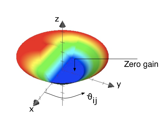
Figure 5: Gain function used to avoid that the positions of two power generators can coincide.

Thus, we modify control law (20) as follows:

$$\begin{split}\dot{w}_{i}&=-\frac{\partial\tilde{H}_{V}}{\partial w_{i}}\doteq u_{i}^{\text{cent,w}},\\ \dot{g}_{i}&=\frac{2}{\pi}\arctan\left[\frac{\|v_{-\partial\tilde{H}_{i}}\|^{2}}{\alpha}\right]\,\,\Theta(v_{C,g_{i}}\cdot v_{-\partial\tilde{H}_{i}})\,\,v_{C,g_{i}}\,\,\prod_{g_{j}\in M_{i}(G,\Delta)}\psi\Bigl{(}\|g_{j}-g_{i}\|,\,\,\vartheta_{ij}\Bigr{)}\doteq u_{i}^{\text{cent,g}}.\end{split}$$ (22)

If $M_{i}(G,\Delta)$ is the empty set, then we have an empty product, whose numerical value is $1$. Notice that the right hand side of (22) is Lipschitz continuous, since it is a product of $C^{1}$ functions and Lipschitz continuous functions, and it can be still computed in a spatially-distributed way (in fact, it only depends on generators that are neighbors in the power diagram, and whose positions are within a distance $\Delta$). One can prove the following result.

Theorem VI.2

Consider the vector field on $\tilde{S}$ defined by equation (22). Then generators’ positions and weights starting at $t=0$ at $G_{W}(0)\in\tilde{S}$, and evolving under (22) remain in $\tilde{S}$ and converge asymptotically to the set of critical points of the primary objective function $\tilde{H}_{V}$ (i.e., to the set of vectors of generators’ positions and weights that yield an equitable power diagram).

Proof:

The proof is virtually identical to the one of Theorem V.9, and we omit it in the interest of brevity. We only notice that $\tilde{H}_{V}$ is non-increasing along system trajectories

$$\dot{\tilde{H}}_{V}=\sum_{i=1}^{m}\frac{\partial\tilde{H}_{V}}{\partial g_{i}}\cdot\dot{g}_{i}+\frac{\partial\tilde{H}_{V}}{\partial w_{i}}\dot{w}_{i}=\sum_{i=1}^{m}\underbrace{\frac{\partial\tilde{H}_{V}}{\partial g_{i}}\cdot\dot{g}_{i}}_{\leq 0}-\Bigl{(}\frac{\partial\tilde{H}_{V}}{\partial w_{i}}\Bigr{)}^{2}\leq 0.$$

Moreover, the components of the vector field (22) for the position of each generator are either zero or point toward $A$ (since the centroid of a cell must be within $A$); therefore, each generator will remain within the compact set $A$. ∎

VI-B Obtaining Power Diagrams “Close” to Voronoi Diagrams

In some applications it could be preferable to have power diagrams as close as possible to Voronoi diagrams. This issue is of particular interest for the setting with non-uniform density, when an equitable Voronoi diagram could fail to exist. The objective of obtaining a power diagram close to a Voronoi diagram can be translated in the minimization of the function $K:{\mathbb{R}}^{m}\to{\mathbb{R}}_{\geq 0}$:

$$K(W)\doteq\frac{1}{2}\sum_{i=1}^{m}w_{i}^{2};$$

when $w_{i}=0$ for all $i\in I_{m}$, we have $K=0$ and the corresponding power diagram coincides with a Voronoi diagram. To include the minimization of the secondary objective $K$, it is natural to consider, instead of (17), the following update law for the weights:

$$\dot{w}_{i}=-\frac{\partial{H}_{V}}{\partial w_{i}}-\frac{\partial K}{\partial w_{i}}=-\frac{\partial{H}_{V}}{\partial w_{i}}-w_{i}.$$ (23)

However, $H_{V}$ is no longer a valid Lyapunov function for system (23). The idea, then, is to let the positions of the generators move so that $\frac{\partial\tilde{H}_{V}}{\partial g_{i}}\cdot\dot{g}_{i}-\frac{\partial\tilde{H}_{V}}{\partial w_{i}}\frac{\partial K}{\partial w_{i}}=0$. In other words, the dynamics of generators’ positions is used to compensate the effect of the term $-w_{i}$ (present in the weights’ dynamics) on the time derivative of $\tilde{H}_{V}$.

Thus, we set up the following control law, with $\varepsilon_{1},\,\varepsilon_{2}$ and $\varepsilon_{3}$ positive small constants, $\varepsilon_{2}>\varepsilon_{1}$,

$$\begin{split}\dot{w}_{i}&=-\frac{\partial\tilde{H}_{V}}{\partial w_{i}}-w_{i}\text{sat}_{\varepsilon_{1},\varepsilon_{2}}\Bigl{(}\|v_{\partial\tilde{H}_{i}}\|\Bigr{)}\,\text{sat}_{0,\varepsilon_{3}}\Bigl{(}\text{dist}(g_{i},\partial V_{i})\Bigr{)},\\ \dot{g}_{i}&=w_{i}\frac{\partial\tilde{H}_{V}}{\partial w_{i}}\frac{v_{\partial\tilde{H}_{i}}}{\|\ v_{\partial\tilde{H}_{i}}\|^{2}}\,\text{sat}_{\varepsilon_{1},\varepsilon_{2}}\Bigl{(}\|v_{\partial\tilde{H}_{i}}\|\Bigr{)}\,\text{sat}_{0,\varepsilon_{3}}\Bigl{(}\text{dist}(g_{i},\partial V_{i})\Bigr{)}.\end{split}$$ (24)

The gain $\text{sat}_{\varepsilon_{1},\varepsilon_{2}}\Bigl{(}\|v_{\partial\tilde{H}_{i}}\|\Bigr{)}$ is needed to make the right hand side of (24) Lipschitz continuous, while the gain $\text{sat}_{0,\varepsilon_{3}}\Bigl{(}\text{dist}(g_{i},\partial V_{i})\Bigr{)}$ avoids that generators’ positions can leave the workspace. Notice that the computation of the right hand side of (24) is spatially distributed over the power-Delaunay graph.

As before, it is possible that under control law (24) there exists a time $t^{*}$ and $i,j\in I_{m}$ such that $g_{i}(t^{*})=g_{j}(t^{*})$. Thus, similarly as before, we modify the update equations (24) as follows

$$\begin{split}\dot{w}_{i}&=-\frac{\partial\tilde{H}_{V}}{\partial w_{i}}-w_{i}\text{sat}_{\varepsilon_{1},\varepsilon_{2}}\Bigl{(}\|v_{\partial\tilde{H}_{i}}\|\Bigr{)}\,\text{sat}_{0,\varepsilon_{3}}\Bigl{(}\text{dist}(g_{i},\partial V_{i})\Bigr{)}\cdot\prod_{g_{j}\in M_{i}(G,\Delta)}\psi\Bigl{(}\|g_{j}-g_{i}\|,\,\,\vartheta_{ij}\Bigr{)}\doteq u_{i}^{\text{vor,w}},\\ \dot{g}_{i}&=w_{i}\frac{\partial\tilde{H}_{V}}{\partial w_{i}}\frac{v_{\partial\tilde{H}_{i}}}{\|\ v_{\partial\tilde{H}_{i}}\|^{2}}\text{sat}_{\varepsilon_{1},\varepsilon_{2}}\Bigl{(}\|v_{\partial\tilde{H}_{i}}\|\Bigr{)}\,\text{sat}_{0,\varepsilon_{3}}\Bigl{(}\text{dist}(g_{i},\partial V_{i})\Bigr{)}\cdot\prod_{g_{j}\in M_{i}(G,\Delta)}\psi\Bigl{(}\|g_{j}-g_{i}\|,\,\,\vartheta_{ij}\Bigr{)}\doteq u_{i}^{\text{vor,g}},\end{split}$$ (25)

where $\vartheta_{ij}$ is defined as in Section VI-A, with $w_{i}\frac{\partial\tilde{H}_{V}}{\partial w_{i}}v_{\partial\tilde{H}_{i}}$ replacing $v_{C,g_{i}}$.

One can prove the following result.

Theorem VI.3

Consider the vector field on $\tilde{S}$ defined by equation (25). Then generators’ positions and weights starting at $t=0$ at $G_{W}(0)\in\tilde{S}$, and evolving under (25) remain in $\tilde{S}$ and converge asymptotically to the set of critical points of the primary objective function $\tilde{H}_{V}$ (i.e., to the set of vectors of generators’ positions and weights that yield an equitable power diagram).

Proof:

Consider $\tilde{H}_{V}$ as a Lyapunov function candidate. First, we prove that set $\tilde{S}$ is positively invariant with respect to (25). Indeed, by definition of (25), we have $g_{i}\neq g_{j}$ for $i\neq j$ for all $t\geq 0$ (therefore, the power diagram is always well defined). Moreover, it is straightforward to see that $\dot{\tilde{H}}_{V}\leq 0$. Therefore, it holds

$$\lambda_{V_{i}(G_{W}(t))}^{-1}\leq\tilde{H}_{V}(G_{W}(t))\leq\tilde{H}_{V}(G_{W}(0)),\quad i\in I_{m},\,\,t\geq 0.$$

Since the measures of the power cells depend continuously on generators’ positions and weights, we conclude that the measures of all power cells will be bounded away from zero. Finally, since $\dot{g}_{i}=0$ on the boundary of $A$ for all $i\in I_{m}$, each generator will remain within the compact set $A$. Thus, generators’ positions and weights will belong to $\tilde{S}$ for all $t\geq 0$, that is, $G_{W}(t)\in\tilde{S}$ $\forall t\geq 0$.

Second, as shown before, $\tilde{H}_{V}:\tilde{S}\to{\mathbb{R}}_{\geq 0}$ is non-increasing along system trajectories, i.e., $\dot{\tilde{H}}_{V}(G_{W})\leq 0$ in $\tilde{S}$.

Third, all trajectories with initial conditions in $\tilde{S}$ are bounded. Indeed, we have already shown that each generator remains within the compact set $A$ under control law (25). As far as the weights are concerned, we start by noticing that the time derivative of the sum of the weights is

$$\frac{\partial\sum_{i=1}^{m}w_{i}}{\partial t}=-\sum_{i=1}^{m}w_{i}\text{sat}_{\varepsilon_{1},\varepsilon_{2}}\Bigl{(}\|v_{\partial\tilde{H}_{i}}\|\Bigr{)}\,\text{sat}_{0,\varepsilon_{3}}\Bigl{(}\text{dist}(g_{i},\partial V_{i})\Bigr{)}\prod_{g_{j}\in M_{i}(G,\Delta)}\psi\Bigl{(}\|g_{j}-g_{i}\|,\,\,\vartheta_{ij}\Bigr{)},$$

since, similarly as in the proof of Theorem V.9, $\sum_{i=1}^{m}\frac{\partial\tilde{H}_{V}}{\partial w_{i}}=0$. Moreover, the magnitude of the difference between any two weights is bounded by a constant, that is,

$$|w_{i}-w_{j}|\leq\alpha\quad\text{for all}\,\,i,\,j\in I_{m};$$ (26)

if, by contradiction, the magnitude of the difference between any two weights could become arbitrarily large, the measure of at least one power cell would vanish, since the positions of the generators are confined within $A$. Assume, by the sake of contradiction, that weights’ trajectories are unbounded. This means that

$$\forall R>0\quad\exists t\,\geq 0\,\,\text{and}\,\,\exists\,j\in I_{m}\quad\text{such that}\quad|w_{j}(t)|\geq R.$$

For simplicity, assume that $w_{i}(0)=0$ for all $i\in I_{m}$ (the extension to arbitrary initial conditions in $\tilde{S}$ is straightforward). Choose $R=2m\alpha$ and let $t_{2}$ be the time instant such that $|w_{j}(t_{2})|=R$, for some $j\in I_{m}$. Without loss of generality, assume that $w_{j}(t_{2})>0$. Because of constraint (26), we have $\sum_{i=1}^{m}w_{i}(t_{2})\geq\frac{\alpha}{2}m(3m+1)$. Let $t_{1}$ be the last time before $t_{2}$ such that $w_{j}(t)=m\alpha$; because of continuity of trajectories, $t_{1}$ is well-defined. Then, because of constraint (26), we have (i) $\sum_{i=1}^{m}w_{i}(t_{1})\leq\frac{\alpha}{2}m(3m-1)<\sum_{i=1}^{m}w_{i}(t_{2})$, and (ii) $\frac{\partial\sum_{i=1}^{m}w_{i}(t)}{\partial t}\leq 0$ for $t\in[t_{1},\,t_{2}]$ (since $w_{j}(t)\geq m\alpha$ for all $t\in[t_{1},\,t_{2}]$ and Eq. (26) imply $\min_{i\in I_{m}}w_{i}(t)>0$ for all $t\in[t_{1},\,t_{2}]$); thus, we get a contradiction.

Finally, by Theorem VI.1, $\tilde{H}_{V}$ is continuously differentiable in $\tilde{S}$. Hence, by invoking the LaSalle invariance principle (see, for instance, [6]), under the descent flow (25), generators’ positions and weights will converge asymptotically to the set of critical points of $\tilde{H}_{V}$, that is not empty by Theorem V.1. ∎

VI-C Obtaining Cells Similar to Regular Polygons

In many applications, it is preferable to avoid long and thin subregions. For example, in applications where a mobile agent has to service demands distributed in its own subregion, the maximum travel distance is minimized when the subregion is a circle. Thus, it is of interest to have subregions whose shapes show circular symmetry, i.e., that are similar to regular polygons.

Define, now, the distortion function $L_{V}:(A\times{\mathbb{R}})^{m}\setminus\Gamma_{\text{coinc}}\mapsto{\mathbb{R}}_{\geq 0}$: $\sum_{i=1}^{m}\int_{V_{i}}\|x-g_{i}\|^{2}\lambda(x)dx$ (where $V_{i}$ is the $i$-th cell in the corresponding power diagram). In [18] it is shown that, when $m$ is large, for the centroidal Voronoi diagram (i.e., centroidal power diagram with equal weights) that minimizes $L_{V}$, all cells are approximately congruent to a regular hexagon, i.e., to a polygon with considerable circular symmetry (see Section VII for a more in-depth discussion about circular symmetry).

Indeed, it is possible to obtain a power diagram that is close to a centroidal Voronoi diagram by combining control laws (22) and (25). In particular, we set up the following (spatially-distributed) control law:

$$\begin{split}\dot{w}_{i}=&u_{i}^{\text{cent,w}}+u_{i}^{\text{vor,w}},\\ \dot{g}_{i}=&u_{i}^{\text{cent,g}}+u_{i}^{\text{vor,g}}.\end{split}$$ (27)

Combining the results of Theorem VI.2 and Theorem VI.3, we argue that with control law (27) it is possible to obtain equitable power diagrams with cells similar to regular polygons, i.e. that show circular symmetry.

VII Simulations and Discussion

In this section we verify through simulation the effectiveness of the optimization for the secondary objectives. Due to space constraints, we discuss only control law (27). We introduce two criteria to judge, respectively, closeness to a Voronoi diagram, and circular symmetry of a partition.

VII-A Closeness to Voronoi Diagrams

In a Voronoi diagram, the intersection between the bisector of two neighboring generators $g_{i}$ and $g_{j}$, and the line segment joining $g_{i}$ and $g_{j}$ is the midpoint $g_{ij}^{\text{vor}}\doteq(g_{i}+g_{j})/2$. Then, if we define $g_{ij}^{\text{pow}}$ as the intersection, in a power diagram, between the bisector of two neighboring generators $(g_{i},w_{i})$ and $(g_{j},w_{j})$ and the line segment joining their positions $g_{i}$ and $g_{j}$, a possible way to measure the distance $\eta$ of a power diagram from a Voronoi diagram is the following:

$$\eta\doteq\frac{1}{2N}\sum_{i=1}^{m}\sum_{j\in N_{i}}\frac{\|g_{ij}^{\text{pow}}-g_{ij}^{\text{vor}}\|}{0.5\,\gamma_{ij}},$$ (28)

where $N$ is the number of neighboring relationships and, as before, $\gamma_{ij}=\|g_{j}-g_{i}\|$. Clearly, if the power diagram is also a Voronoi diagram (i.e., if all weights are equal), we have $\eta=0$. We will also refer to $\eta$ as the Voronoi defect of a power diagram.

VII-B Circular Symmetry of a Partition

A quantitative manifestation of circular symmetry is the well-known isoperimetric inequality which states that among all planar objects of a given perimeter, the circle encloses the largest area. More precisely, given a planar region $V$ with perimeter $p_{V}$ and area $|V|$, then $p_{V}^{2}-4\pi|V|\geq 0$, and equality holds if and only if $V$ is a circle. Then, we can define the isoperimetric ratio as follows: $Q_{V}=\frac{4\pi|V|}{p_{V}^{2}}$; by the isoperimetric inequality, $Q_{V}\leq 1$, with equality only for circles. Interestingly, for a regular $n$-gon the isoperimetric ratio $Q_{n}$ is $Q_{n}=\frac{\pi}{n\tan\frac{\pi}{n}}$, which converges to $1$ for $n\to\infty$. Accordingly, given a partition $\mathcal{A}=\{A_{i}\}_{i=1}^{m}$, we define, as a measure for the circular symmetry of the partition, the isoperimetric ratio $Q_{\mathcal{A}}\doteq\frac{1}{m}\sum{Q_{A_{i}}}$.

VII-C Simulation Results

We simulate ten agents providing service in the unit square $A$. Agents’ initial positions are independently and uniformly distributed over $A$, and all weights are initialized to zero. Time is discretized with a step $dt=0.01$, and each simulation run consists of $800$ iterations (thus, the final time is $T=8$). Define the area error $\epsilon$ as the difference, at $T=8$, between the measure of the region of dominance with maximum measure and the measure of the region of dominance with minimum measure.

First, we consider a measure $\lambda$ uniform over $A$, in particular $\lambda\equiv 1$. Therefore, we have $\lambda_{A}=1$ and agents should reach a partition in which each region of dominance has measure equal to $0.1$. For this case, we run $50$ simulations.

Then, we consider a measure $\lambda$ that follows a gaussian distribution, namely $\lambda(x,y)=e^{-5((x-0.8)^{2}+(y-0.8)^{2})}$, $(x,y)\in A$, whose peak is at the north-east corner of the unit square. Therefore, we have $\lambda_{A}\approx 0.336$, and vehicles should reach a partition in which each region of dominance has measure equal to $0.0336$. For this case, we run $20$ simulations.

Table I summarizes simulation results for the uniform $\lambda$ ($\lambda$=unif) and the gaussian $\lambda$ ($\lambda$=gauss). Expectation and worst case values of area error $\epsilon$, Voronoi defect $\eta$ and isoperimetric ratio $Q_{\mathcal{V}}$ are with respect to $50$ runs for uniform $\lambda$, and $20$ runs for gaussian $\lambda$. Notice that for both measures, after $800$ iterations, (i) the worst case area error is within $16\%$ from the desired measure of dominance regions, (ii) the worst case $\eta$ is very close to $0$, and, finally, (iii) cells have, approximately, the circular symmetry of squares (since $Q_{4}\approx 0.78$). Therefore, convergence to a convex equitable partition with the desired properties (i.e., closeness to Voronoi diagrams and circular symmetry) seems to be robust. Figure 6 shows the typical equitable partitions that are achieved with control law (27) with $10$ agents.

TABLE I: Performance of control law (27).

$\lambda$	$\mathbb{E}\left[\epsilon\right]$	$\max\epsilon$	$\mathbb{E}\left[\eta\right]$	$\max\eta$	$\mathbb{E}\left[Q_{\mathcal{V}}\right]$	$\min Q_{\mathcal{V}}$
unif	$3.8\,10^{-4}$	$0.016$	$0.01$	$0.03$	$0.73$	$0.66$
gauss	$3\,10^{-3}$	$5.3\,10^{-3}$	$0.02$	$0.04$	$0.75$	$0.69$

  

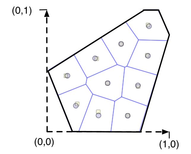
(a) Typical equitable partition of $A$ for $\lambda(x,y)=1$.

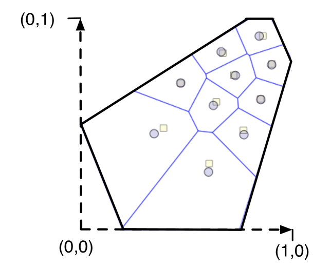
(b) Typical equitable partition of $A$ for $\lambda(x,y)=e^{-5((x-0.8)^{2}+(y-0.8)^{2})}$.

Figure 6: Typical equitable partitions achieved by using control law (27). The yellow squares represent the position of the generators, while the blue circles represent the centroids. Notice how each bisector intersects the line segment joining the two corresponding power neighbors almost at the midpoint; hence both partitions are very close to Voronoi partitions. Compare with Fig. 2.

VIII Application and Conclusion

In this last section, we present an application of our algorithms and we draw our conclusions.

VIII-A Application

A possible application of our algorithms is in the Dynamic Traveling Repairman Problem (DTRP). In the DTRP, $m$ agents operating in a workspace $A$ must service demands whose time of arrival, location and on-site service are stochastic; the objective is to find a policy to service demands over an infinite horizon that minimizes the expected system time (wait plus service) of the demands. There are many practical settings in which such problem arises. Any distribution system which receives orders in real time and makes deliveries based on these orders (e.g., courier services) is a clear candidate. Equitable partitioning policies (with respect to a suitable measure $\lambda$ related to the probability distribution of demand locations) are, indeed, optimal for the DTRP when the arrival rate for service demands is large enough (see [1, 19, 20]). Therefore, it is of interest to combine the optimal equitable partitioning policies in [19] with the spatially-distributed algorithms presented in this paper.

The first step is to associate to each agent $i$ a virtual power generator (virtual generator for short) $(g_{i},w_{i})$. We define the region of dominance for agent $i$ as the power cell $V_{i}=V_{i}(G_{W})$, where $G_{W}=\Bigl{(}(g_{1},w_{1}),\cdots,(g_{m},w_{m})\Bigr{)}$ (see Fig. 7(a)). We refer to the partition into regions of dominance induced by the set of virtual generators $G_{W}$ as $\mathcal{V}(G_{W})$. A virtual generator $(g_{i},w_{i})$ is simply an artificial variable locally controlled by the $i$-th agent; in particular, $g_{i}$ is a virtual point and $w_{i}$ is its weight. Virtual generators allow us to decouple the problem of achieving an equitable partition into regions of dominance from that of positioning an agent inside its own region of dominance.

Then, each agent applies to its virtual generator one of the previous algorithms, while it performs inside its region of dominance the optimal single-agent policy described in [1] (see Fig. 7(b)).

  

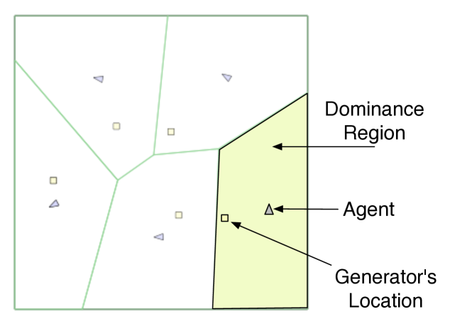
(a) Agents, virtual generators and regions of dominance.

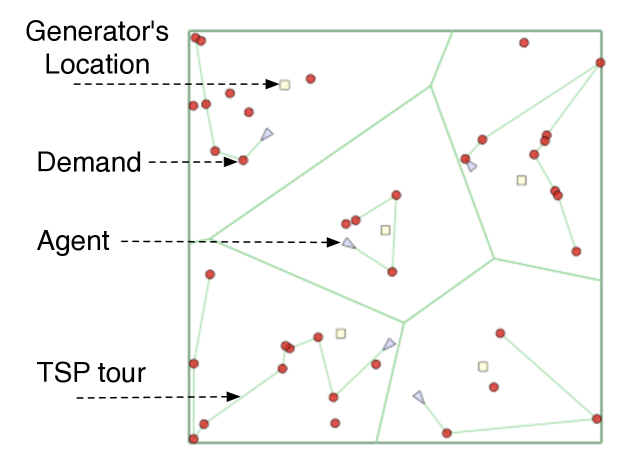
(b) Each agent services outstanding demands inside its own region of dominance.

Figure 7: Spatially-distributed algorithms for the DTRP.

Notice that, since each agent is required to travel inside its own region of dominance, this scheme is inherently safe against collisions.

VIII-B Conclusion

We have presented provably correct, spatially-distributed control policies that allow a team of agents to achieve a convex and equitable partition of a convex workspace. We also considered the issue of achieving convex and equitable partitions with special properties (e.g., with hexagon-like cells). Our algorithms could find applications in many problems, including dynamic vehicle routing, and wireless networks. This paper leaves numerous important extensions open for further research. First, all the algorithms that we proposed are synchronous: we plan to devise algorithms that are amenable to asynchronous implementation. Second, we envision considering the setting of structured environments (ranging from simple nonconvex polygons to more realistic ground environments). Finally, to assess the closed-loop robustness and the feasibility of our algorithms, we plan to implement them on a network of unmanned aerial vehicles.

Appendix

Proof:

The proof mainly relies on [21]. Let $v$ be the unit vector considered in the definition of the Unimodal Property. Then, there exist unique values $s_{0}<s_{1}<\cdots<s_{m}$ such that $s_{0}=\inf\{s;A^{s}\neq\emptyset\}$, $s_{m}=\sup\{s;A^{s}\neq\emptyset\}$, and

$$\lambda_{\{x\in A;\,v\cdot x\leq s_{k}\}}=\frac{k}{m}\lambda_{A},\quad k=1,\ldots,m-1.$$ (29)

Consider the intervals $I_{i}\doteq[s_{i-1},s_{i}]$, $i\in I_{m}.$ We claim that one can choose points $g_{i}=t_{i}v\in{\mathbb{R}}^{d}$, $i\in I_{m}$ such that $t_{i}\in I_{i}$ and the corresponding Voronoi diagram is

$$\begin{split}A_{i}&=\{x\in A;\quad\|x-g_{i}\|=\min_{k}\|x-g_{k}\|\}\\ &=\{x\in A;\quad v\cdot x\in[s_{i-1},s_{i}]\}.\end{split}$$ (30)

Together, Eq. (29) and Eq. (30) yield the desired result.

Since, by assumption, $A$ enjoys the Unimodal Property, there exists an index $\kappa\in\{1,\ldots,m\}$ such that the length of the intervals $I_{i}=[s_{i-1},s_{i}]$ decreases as $i$ ranges from $1$ to $\kappa$, then increases as $i$ ranges from $\kappa$ to $m$. Let $I_{\kappa}=[s_{\kappa-1},s_{\kappa}]$ be the smallest of these intervals, and define

$$t_{\kappa}\doteq\frac{s_{\kappa-1}+s_{\kappa}}{2}\in I_{\kappa}.$$

By induction, for $i$ increasing from $\kappa$ to $m-1$, define $t_{i+1}$ be the symmetric to $t_{i}$ with respect to $s_{i}$, so that

$$t_{i+1}=2s_{i}-t_{i}\quad i=\kappa,\kappa+1,\ldots,m-1.$$

Since the length of $I_{i+1}$ is larger than the length of $I_{i}$, we have

$$t_{i}\in I_{i}\Rightarrow t_{i+1}\in I_{i+1}.$$ (31)

Similarly, for $i$ decreasing from $\kappa$ to $1$, we define

$$t_{i-1}=2s_{i-1}-t_{i},\quad i=\kappa,\kappa-1,\ldots,2.$$

Since the interval $I_{i-1}$ is now larger than the interval $I_{i}$, we have

$$t_{i}\in I_{i}\Rightarrow t_{i-1}\in I_{i-1}.$$ (32)

By Eqs. (31)-(32) imply $t_{i}\in I_{i}$ for all $i=1,\ldots,m$. Hence the second equality in Eq. (30) holds. ∎

We now specialize the theorem to the case when $A$ is convex.

Corollary VIII.1

Let $A\subset{\mathbb{R}}^{d}$ be a compact, convex set, and $\lambda$ be constant on $A$. Then for every $m\geq 1$ there exist points $g_{1},\cdots,g_{m}$ all in the interior of $A$, such that the corresponding Voronoi diagram is equitable.

Proof:

Notice that every compact convex set enjoys the Unimodal Property, with an arbitrary choice of the unit vector $v$. By compactness, there exist points $a,\,b\in A$ such that $\|b-a\|=\max_{z,z^{\prime}\in A}\|z-z^{\prime}\|.$ By a translation of coordinates, we can assume $a$ = 0. Choose $v\doteq b/\|b\|$. Then the previous construction yields an equitable Voronoi diagram generated by $m$ points $g_{i}=t_{i}v$ all in the interior of $A$. ∎

Proof:

By Theorem V.9 and by its very definition $W^{*}(G)$ is the zero of the vector field $-\frac{\partial H_{V}}{\partial w_{i}}(W(t))$. Now let us denote with

$$K(W,G)\dot{=}-\frac{\partial H_{V}}{\partial w_{i}}(W),$$

the corresponding continuous function, viewed as a function of two independent set of variables, namely the weights $(w_{1},\dots,w_{n})=W$ and the non-degenerate vector of generators’ locations $G$. In order to prove that the assignment $G\mapsto W^{*}(G)$ is continuous, notice that by Theorem V.6 the function $K(W,G)$ is identically zero when restricted to the graph of $W^{*}$, namely $K(W^{*}(G),G)=0$. The function $W^{*}$ is continuous iff it is continuous in each of its argument. Fix, first, a generator $g_{i}\notin\partial\Gamma$ and consider for any $v\in\mathbb{R}^{2}$, the variation $(g_{1},\dots,g_{i-1},g_{i}+hv,g_{i+1},\dots,g_{m})$. Since $g_{i}\notin\partial\Gamma$, there always exists an $\epsilon>0$, depending on $g_{i}$ and $v$, such that for any $h$ with $0\leq h<\epsilon$, $(g_{1},\dots,g_{i-1},g_{i}+hv,g_{i+1},\dots,g_{m})\in\Gamma$. Now $K(W^{*}(g_{1},\dots,g_{i-1},g_{i}+hv,g_{i+1},\dots,g_{m}),(g_{1},\dots,g_{i-1},g_{i}+hv,g_{i+1},\dots,g_{m}))=0$ for any $0\leq h<\epsilon$ by definition. Therefore, taking the limit for $h\rightarrow 0^{+}$, we still get zero. On the other hand, since $K$ is continuous, we can take the limit inside $K$ and we get

$$K(\lim_{h\rightarrow 0^{+}}W^{*}(g_{1},\dots,g_{i-1},g_{i}+hv,g_{i+1},\dots),(g_{1},\dots,g_{i-1},g_{i},g_{i+1},\dots))=0.$$

Therefore, we have that $\lim_{h\rightarrow 0^{+}}W^{*}(g_{1},\dots,g_{i-1},g_{i}+hv,g_{i+1},\dots,g_{m})$ is equal to $W^{*}(g_{1},\dots,g_{i-1},g_{i},g_{i+1},\dots,g_{m})$, by the uniqueness in $\Omega$ of the value of $W^{*}$ for which, given $G$, the function $K$ vanishes. ∎

References

- [1] D. J. Bertsimas and G. J. van Ryzin, “Stochastic and dynamic vehicle routing in the Euclidean plane with multiple capacitated vehicles,” Advances in Applied Probability, vol. 25, no. 4, pp. 947–978, 1993.
- [2] O. Baron, O. Berman, D. Krass, and Q. Wang, “The equitable location problem on the plane,” European Journal of Operational Research, vol. 183, no. 2, pp. 578–590, 2007.
- [3] B. Liu, Z. Liu, and D. Towsley, “On the capacity of hybrid wireless networks,” in IEEE INFOCOM 2003, San Francisco, CA, Apr. 2003, pp. 1543–1552.
- [4] J. Carlsson, D. Ge, A. Subramaniam, A. Wu, and Y. Ye, “Solving min-max multi-depot vehicle routing problem,” Report, 2007.
- [5] S. P. Lloyd, “ Least-squares quantization in PCM,” IEEE Trans. Information Theory, vol. 28, no. 2, pp. 129–137, 1982.
- [6] F. Bullo, J. Cortés, and S. Martínez, Distributed Control of Robotic Networks, ser. Applied Mathematics Series. Princeton University Press, Sep. 2008, manuscript under contract. Electronically available at http://coordinationbook.info.
- [7] A. Kwok and S. Martinez, “Energy-balancing cooperative strategies for sensor deployment,” in Proc. IEEE Conf. on Decision and Control, New Orleans, LA, Dec. 2007, pp. 6136–6141.
- [8] J. Carlsson, B. Armbruster, and Y. Ye, “Finding equitable convex partitions of points in a polygon efficiently,” To appear in The ACM Transactions on Algorithms, 2008.
- [9] R. Diestel, Graph Theory, 2nd ed., ser. Graduate Texts in Mathematics. New York: Springer Verlag, 2000, vol. 173.
- [10] I. Chavel, Eigenvalues in Riemannian Geometry. New York, NY: Academic Press, 1984.
- [11] A. Hatcher, Algebraic Topology. Cambridge, U.K.: Cambridge University Press, 2002. [Online]. Available: http://www.math.cornell.edu/hatcher/AT/ATpage.html
- [12] A. Okabe, B. Boots, K. Sugihara, and S. N. Chiu, Spatial Tessellations: Concepts and Applications of Voronoi Diagrams. New York, NY: John Wiley & Sons, 2000.
- [13] H. Imai, M. Iri, and K. Murota, “Voronoi diagram in the Laguerre geometry and its applications,” SIAM Journal on Computing, vol. 14, no. 1, pp. 93–105, 1985.
- [14] F. Aurenhammer, “Power diagrams: properties, algorithms and applications,” SIAM Journal on Computing, vol. 16, no. 1, pp. 78–96, 1987.
- [15] J. Cortés, S. Martínez, and F. Bullo, “Spatially-distributed coverage optimization and control with limited-range interactions,” ESAIM. Control, Optimisation & Calculus of Variations, vol. 11, pp. 691–719, 2005.
- [16] M. Pavone, E. Frazzoli, and F. Bullo, “Decentralized algorithms for stochastic and dynamic vehicle routing with general demand distribution,” in Proc. IEEE Conf. on Decision and Control, New Orleans, LA, Dec. 2007, pp. 4869–4874.
- [17] ——, “Distributed policies for equitable partitioning: Theory and applications,” in Proc. IEEE Conf. on Decision and Control, Cancun, Mexico, Dec. 2008.
- [18] D. Newman, “The hexagon theorem,” IEEE Transactions on Information Theory, vol. 28, no. 2, pp. 137–139, Mar 1982.
- [19] D. J. Bertsimas and G. J. van Ryzin, “Stochastic and dynamic vehicle routing with general interarrival and service time distributions,” Advances in Applied Probability, vol. 25, pp. 947–978, 1993.
- [20] H. Xu, “Optimal policies for stochastic and dynamic vehicle routing problems.” Dept. of Civil and Environmental Engineering, Massachusetts Institute of Technology, Cambridge, MA., 1995.
- [21] A. Bressan, Personal Communication, 2008.