Projection Operator Approach to Transport in Complex Single-Particle Quantum Systems

Abstract

We discuss the time-convolutionless (TCL) projection operator approach to transport in closed quantum systems. The projection onto local densities of quantities such as energy, magnetization, particle number, etc. yields the reduced dynamics of the respective quantities in terms of a systematic perturbation expansion. In particular, the lowest order contribution of this expansion is used as a strategy for the analysis of transport in “modular” quantum systems corresponding to quasi one-dimensional structures which consist of identical or similar many-level subunits. Such modular quantum systems are demonstrated to represent many physical situations and several examples of complex single-particle models are analyzed in detail. For these quantum systems lowest order TCL is shown to represent an efficient tool which also allows to investigate the dependence of transport on the considered length scale. To estimate the range of validity of the obtained equations of motion we extend the standard projection to include additional degrees of freedom which model non-Markovian effects of higher orders.

1 Introduction

In recent years the application of projection operator techniques nakajima1958 ; zwanzig1960 ; chaturvedi1979 ; breuer2007 ; breuer2006 ; breuer2007b to transport investigations in (closed) quantum systems has been suggested steinigeweg2007-1 ; weimer2008 ; wu2008 . Within these approaches a suitable projection onto local densities of pertinent transport quantities is used in order to obtain the reduced dynamics of these quantities in terms of a systematic perturbation expansion, typically w.r.t. some (small) interaction strength. For certain examples the lowest order contribution of this expansion has been shown to yield reliable predictions on transport weimer2008 as well as on its length scale dependence steinigeweg2007-1 .

However, the lowest order truncation may become questionable for strongly interacting quantum systems, of course. But already in the weak coupling case the validity of this truncation generally is restricted to short time scales bartsch2008 . This fact seems to be problematic, especially since the relevant time scale can be very long for small interaction strengths or large length scales steinigeweg2007-1 , e. g., in the thermodynamic limit. For this reason the additional consideration of higher order contributions appears to be indispensable breuer2006 , contrary to the statements in, e. g., Ref. wu2008 . Because such a consideration has not been provided in the literature so far, the main intention of the present paper is the incorporation of higher order terms as well, particularly the next-to-lowest order contribution.

To start with we will introduce the notion of a modular quantum system in Sec. 2. Modular quantum systems are demonstrated to represent many physical situations and several examples will be given. In the context of these quantum systems the time-convolutionless (TCL) projection operator technique chaturvedi1979 ; breuer2006 ; breuer2007 is subsequently discussed. In Sec. 3 the projection onto local densities and lowest order TCL is firstly shown as an appropriate method which also allows to investigate the dependence of transport on the considered length scale. In particular explicit conditions for the applicability of the introduced method are given. The next Sec. 4 is concerned with the higher order contributions of the TCL expansion and a suitable estimation is derived for the special case of interactions with van Hove structure vanhove1954 ; vanhove1957 ; bartsch2008 . In Sec. 5 this estimation is used in order to determine the range of validity of lowest order TCL and an interpretation in the context of length scales is provided. Section 6 finally applies the concepts of the previous Sections to complex single-particle models, e. g., to models with disorder. Our results are confirmed by numerical solution of the full time-dependent Schrödinger equation.

2 Modular Quantum Systems and Diffusive Dynamics

In the present paper we consider so-called “modular” quantum systems which have a quasi one-dimensional structure and consist of $N$ identical or at least similar many-level subunits. These subunits are described by a local Hamiltonian $\hat{h}_{\mu}$ and the next-neighbor interaction between two adjacent subunits is denoted by $\lambda\,\hat{v}_{\mu,\mu+1}$, where $\lambda$ adjusts the overall coupling strength. The total Hamiltonian $\hat{H}=\hat{H}_{0}+\lambda\,\hat{V}$ is given by

$$\hat{H}_{0}=\sum_{\mu=0}^{N-1}\hat{h}_{\mu}\,,\;\hat{V}=\sum_{\mu=0}^{N-1}\hat{v}_{\mu,\mu+1}\,,$$ (1)

where we employ periodic boundary conditions, i. e., we identify $\mu=N$ with $\mu=0$. Such a description obviously applies to one-dimensional structures such as chains of atoms, molecules, quantum dots, etc. But also $s=1/2$ spin chains fit into this scheme of description, because a segment of the chain, that is, a number of spins and their mutual interactions can be chosen in order to form a suitable many-level subunit. Similarly, spin lattices or higher-dimensional models of the Hubbard type can be treated by the use of (1), if a whole chain (2D) or layer (3D) is considered as a single subunit. Thus, for a large class of quantum systems an adequate way of description is offered by the Hamiltonian of Eq. (1), see Sec. 6 for details.

In this paper we primarily deal with “single-particle” quantum systems, that is, those quantum systems which allow to restrict the investigation to a linearly instead of an exponentially increasing Hilbert space. This is mainly done in order to open the possibility for a comparison of the theoretical predictions with the numerical solution of the full time-dependent Schrödinger equation. Hence, we may suppose

$$\hat{h}_{\mu}=\sum_{i=0}^{n-1}h_{\mu}^{i}\,|\mu,i\rangle\langle\mu,i|\,,$$ (2)

$$\hat{v}_{\mu,\mu+1}=\sum_{i,j=0}^{n-1}v_{\mu,\mu+1}^{i,j}\,|\mu,i\rangle\langle\mu+1,j|+\text{H.c.}\,,$$ (3)

where $n$ denotes the number of levels within a subunit. Without loss of generality, we have additionally assumed an off-diagonal block structure of the interaction, that is, $|\mu,i\rangle$ and $|\mu,j\rangle$ are not coupled.

Of particular interest is the local density $p_{\mu}(t)$ of, e. g., energy, magnetization, excitations, particles, probability, etc. This quantity is expressed as the expectation value of a corresponding operator $\hat{p}_{\mu}$,

$$p_{\mu}(t)=\text{Tr}\{\rho(t)\,\hat{p}_{\mu}\}\,,\;\hat{p}_{\mu}=\sum_{i=0}^{n-1}p_{\mu}^{i}\,|\mu,i\rangle\langle\mu,i|\,,$$ (4)

where $\rho(t)$ is the full system’s density matrix. Since the operators $\hat{p}_{\mu}$ are assumed to be diagonal in the energy representation of the uncoupled system, we restrict ourselves to those quantities $p_{\mu}(t)$ which are conserved for the special case of $\lambda=0$. However, this restriction still allows to investigate transport for a large class of systems, as will be demonstrated in Sec. 6. Our aim is to analyze the dynamical behavior of the $p_{\mu}(t)$ and to develop explicit criteria which enable a clear distinction between diffusive and other available types of transport, e. g., ballistic or insulating behavior.

The dynamical behavior may be called diffusive if the $p_{\mu}(t)$ fulfill a discrete diffusion equation

$$\dot{p}_{\mu}(t)=D\,[\,p_{\mu-1}(t)-2\,p_{\mu}(t)+p_{\mu+1}(t)\,]$$ (5)

with some $\mu$- and $t$-independent diffusion constant $D$. It is straightforward to show [multiplying (5) by $\mu$, respectively $\mu^{2}$, summarizing over $\mu$ and manipulating indices on the r.h.s.] that the spatial variance

$$\sigma^{2}(t)=\sum_{\mu=0}^{N-1}\mu^{2}\,p_{\mu}(t)-\left[\,\sum_{\mu=0}^{N-1}\mu\,p_{\mu}(t)\,\right]^{2}$$ (6)

increases linearly with $t$, namely $\sigma^{2}(t)=2\,D\,t$. By contrast, ballistic behavior is characterized by $\sigma^{2}(t)\propto t^{2}$, whereas insulating behavior corresponds to $\sigma^{2}(t)=\text{const.}$

According to Fourier’s work, diffusions equations are routinely decoupled with respect to, e. g., cosine-shape spatial density profiles

$$p_{q}(t)=C_{q}\sum_{\mu=0}^{N-1}\cos(q\,\mu)\,p_{\mu}(t)\,,\;q=\frac{2\pi\,k}{N}\,,$$ (7)

with $k=0,1,\ldots,N/2$ and a suitable normalization constant $C_{q}$. Consequently, Eq. (5) yields

$$\dot{p}_{q}(t)=-2\,(1-\cos q)\,D\,p_{q}(t)\,.$$ (8)

Therefore, if the quantum model indeed shows diffusive transport, all modes $p_{q}(t)$ have to relax exponentially. If, however, the $p_{q}(t)$ are found to relay exponentially only for some regime of $q$, the model is said to behave diffusively on the corresponding length scale $l=2\pi/q$. One might think of a length scale which is both large compared to some mean free path [below that ballistic behavior occurs, $\sigma^{2}(t)\propto t^{2}$] and small compared to, say, some localization length [beyond that insulating behavior appears, $\sigma^{2}(t)=\text{const.}$], see Sec. 6.

3 Projection onto Local Densities and Second Order TCL

A strategy for the analysis of the dynamical behavior of the $p_{q}(t)$ is provided by the time-convolutionless (TCL) projection operator technique chaturvedi1979 ; breuer2006 ; breuer2007 . This technique, and the well-known Nakajima-Zwanzig (NZ) method as well, are applied in order to describe the reduced dynamics of a quantum system with a Hamiltonian of the form $\hat{H}=\hat{H}_{0}+\lambda\,\hat{V}$, see Refs. nakajima1958 ; zwanzig1960 . Even though projection operator methods are well-established approaches in the context of open systems, the following application to transport in closed systems is a novel concept. Let us remark that the application of these techniques only requires that the pertinent observables commute with $\hat{H}_{0}$.

Generally, the full dynamics of a quantum system is given by the Liouville-von Neumann equation

$$\frac{\partial}{\partial t}\,\rho(t)=-\imath\,[\,\lambda\,\hat{V}(t),\rho(t)\,]={\cal L}(t)\,\rho(t)\,,$$ (9)

where time arguments refer to the interaction picture. In order to describe the reduced dynamics of the system, one has to construct a suitable projection operator $\cal P$ which projects onto the relevant part of the density matrix $\rho(t)$. In particular, $\cal P$ has to satisfy the property ${\cal P}^{2}={\cal P}$. Because in our case the relevant variables are the local densities $p_{\mu}(t)$, we choose

$${\cal P}\,\rho(t)=\sum_{\mu=0}^{N-1}\text{Tr}\{\rho(t)\,\hat{p}_{\mu}\}\,\hat{p}_{\mu}=\sum_{\mu=0}^{N-1}p_{\mu}(t)\,\hat{p}_{\mu}\,.$$ (10)

This choice indeed fulfills the property ${\cal P}^{2}=\cal P$, if we additionally normalize

$$\text{Tr}\{\,(\hat{p}_{\mu})^{2}\,\}=\sum_{i=0}^{n-1}(p_{\mu}^{i})^{2}=1\,,$$ (11)

which can be done without loss of generality. Note that this normalization typically implies $p_{\mu}^{i}\sim 1/\sqrt{n}$, at least for the models in Sec. 6.

Once some projection operator has been defined, the TCL formalism routinely yields [not only for our choice of $\cal P$ in Eq. (10)] a closed and time-local equation for the dynamics of ${\cal P}\,\rho(t)$,

$$\frac{\partial}{\partial t}\,{\cal P}\,\rho(t)={\cal K}(t)\,{\cal P}\,\rho(t)+{\cal I}(t)\,(1-{\cal P})\,\rho(0),$$ (12)

and avoids the often troublesome time-convolution which appears, e. g., in the context of the NZ method. Eq. (12) and, in particular, its time-locality are a standard result and a direct consequence of the TCL formalism chaturvedi1979 ; breuer2006 ; breuer2007 . The time-locality of the TCL equation may be understood as the result of a forward and backward propagation of the corresponding NZ equation in time. In Sec. 6 we will briefly comment on the NZ approach and, especially, on its implications for our class of models.

For initial conditions $\rho(0)$ with ${\cal P}\,\rho(0)=\rho(0)$ the inhomogeneity ${\cal I}(t)$ on the r.h.s. of (12) vanishes. [But for the models in Sec. 6 there are numerical indications that ${\cal I}(t)$ is even negligible for other $\rho(0)$, see also Refs. michel2005 ; breuer2006 ; bartsch2008 .] The generator ${\cal K}(t)$ is given as a systematic perturbation expansion in powers of the coupling strength $\lambda$,

$${\cal K}(t)=\sum_{m=1}^{\infty}\lambda^{m}\,{\cal K}_{m}(t)\,.$$ (13)

The odd contributions of this expansion vanish for many models and for our models as well, that is, ${\cal K}_{2m-1}=0$. Consequently, the lowest non-vanishing contribution is the second order ${\cal K}_{2}(t)$ which reads

$${\cal K}_{2}(t)=\int_{0}^{t}\text{d}t_{1}\,{\cal P}\,{\cal L}(t)\,{\cal L}(t_{1})\,{\cal P}\,.$$ (14)

The next non-vanishing contribution is the fourth order ${\cal K}_{4}(t)$ which is given by

$${\cal K}_{4}(t)\! = \!\int_{0}^{t}\text{d}t_{1}\int_{0}^{t_{1}}\text{d}t_{2}\int_{0}^{t_{2}}\text{d}t_{3}$$ (15)

$$\!\Big{[}{\cal P}\,{\cal L}(t)\,{\cal L}(t_{1})\,(1-{\cal P})\,{\cal L}(t_{2})\,{\cal L}(t_{3})\,{\cal P}$$

$$\!-{\cal P}\,{\cal L}(t)\,{\cal L}(t_{2})\,{\cal P}\,{\cal L}(t_{1})\,{\cal L}(t_{3})\,{\cal P}$$

$$\!-{\cal P}\,{\cal L}(t)\,{\cal L}(t_{3})\,{\cal P}\,{\cal L}(t_{1})\,{\cal L}(t_{2})\,{\cal P}\Big{]}\,.$$

The truncation of the generator (13) to lowest order, i. e., its approximation by the second order (14), is commonly done in the case of small $\lambda$ but is in general restricted to short time scales. As already mentioned in the introduction, this truncation seems to be problematic, since the relevant time scale can be very long, especially if $\lambda$ is small. However, the rest of this Section is only devoted to the second order truncation. In the following Sec. 4 we will additionally discuss the fourth order (15) and subsequently show that its incorporation is indispensable in order to estimate the accuracy of the second order prediction. Moreover, we will demonstrate that some non-diffusive transport phenomena such as localization can not be predicted correctly by a mere second order consideration, see Sec. 6.

Plugging the projector (10) into (12) and (14) leads to

$$\dot{p}_{\mu}(t)=\lambda^{2}\!\!\sum_{\nu=\mu-1}^{\mu+1}\!\!R_{\mu,\nu}(t)\,p_{\nu}(t)\,.$$ (16)

Note that the sum does not run over all $\nu$, because only adjacent subunits are coupled. The time-dependent rates $R_{\mu,\nu}(t)$ are defined by

$$R_{\mu,\nu}(t)=\int_{0}^{t}\text{d}\tau\,C_{\mu,\nu}(\tau)\,,$$ (17)

where we have introduced the correlation functions

$$C_{\mu,\nu}(\tau)=\text{Tr}\Big{\{}[\,\hat{p}_{\mu},\hat{V}(t)\,][\,\hat{p}_{\nu},\hat{V}(t_{1})\,]\Big{\}}\,,\;\tau=t-t_{1}$$ (18)

with $C_{\mu,\nu}(\tau)=C_{\nu,\mu}(\tau)$. [The trace is independent from the order of commutators and time arguments.]

So far, Eq. (16) is exact. For the further simplification of (16) two assumptions have to be made now.
(i.) We assume that $R_{\mu,\mu-1}(t)$, $R_{\mu,\mu}(t)$ and $R_{\mu,\mu+1}(t)$ depend only negligibly on the concrete choice of $\mu$. Hence, it follows that $R_{\mu,\mu-1}(t)\approx R_{\mu+1,\mu}(t)=R_{\mu,\mu+1}(t)$. This is fulfilled exactly, if the system is translational invariant, e. g., if the coefficients in (2), (3) and (4) are the same for each subunit.
(ii.) Moreover, we assume $R_{\mu,\mu-1}(t)\approx-R_{\mu,\mu}(t)/2$. This is perfectly satisfied if the sum of all local densities is conserved since the overall conservation implies

$$\sum_{\nu=0}^{N-1}[\,\hat{p}_{\nu},\hat{V}(t_{1})\,]=0\,.$$ (19)

Consequently, the sum of $C_{\mu,\nu}(\tau)$ over all $\nu$, eventually $2\,C_{\mu,\mu-1}(\tau)+C_{\mu,\mu}(\tau)$, also vanishes.
Due to (i.) and (ii.) the Fourier transform of (16) reads

$$\dot{p}_{q}(t)=-W\,R(t)\,p_{q}(t)\,,\qquad W=2\,(1-\cos q)\,\lambda^{2}$$ (20)

with a single rate $R(t)=-R_{\mu,\mu}(t)/2$. Note that this rate is still time-dependent. Remarkably, the dependence on $q$ and $\lambda$ simply appears as an overall scaling factor $W$.

The models in Sec. 6 typically feature a correlation function $C(\tau)$ which decays completely within some time scale $\tau_{C}$. After this correlation time $C(\tau)$ approximately remains zero and $R(t)$ takes on a constant value $R$, the area under the initial peak of $C(\tau)$. Since the correlation time apparently is independent from $q$ and $\lambda$, it is always possible to realize a relaxation time $\tau_{R}\propto 1/W$ which is much larger than $\tau_{C}$, e. g., in an infinite system there definitely is a small enough $q$. For $\tau_{C}\ll\tau_{R}$ the second order truncation (20) immediately yields

$$\dot{p}_{q}(t)=-W\,R\;p_{q}(t),$$ (21)

and the comparison with (8) clearly indicates diffusive behavior with a diffusion constant $D=\lambda^{2}\,R$.

However, the present method is not restricted to the investigation of diffusive transport phenomena and (20) is applicable as well in order to completely classify the dynamics of $p_{q}(t)$ which decay on relatively short time scales below $\tau_{C}$ or on very long time scales where, e. g., correlations may reappear, see Ref. steinigeweg2007-1 and Sec. 6.

4 Extension of the Projection and Fourth Order TCL

This Section and the next Sec. 5 as well are concerned with the question, why and to what extend the projection onto local densities and second order TCL yield reliable predictions for the dynamical behavior of the $p_{q}(t)$. The answer to this question surely requires the consideration of the higher order contributions of the TCL expansion, e. g., the investigation of the fourth order ${\cal K}_{4}(t)$, cf. (15). But already the direct evaluation of ${\cal K}_{4}(t)$ turns out to be extremely difficult in general, both analytically and numerically. The problem is mainly caused by the first integrand in the expression (15) which significantly contributes to ${\cal K}_{4}(t)$.

We therefore present an alternative approach which is essentially based on the following idea: The influence of the higher order terms may decrease substantially, if the projection additionally incorporates variables which are not of particular interest by themselves but potentially affect the dynamical behavior of the local densities. This idea is obviously only useful if the complexity of the higher order terms decreases to a larger extend than the complexity of the second order contribution increases.

We concretely choose $N\,(n-1)$ additional variables $a_{\mu}^{i}(t)$ which are also given as the expectation values of corresponding operators $\hat{a}_{\mu}^{i}$. These operators are assumed to be diagonal in the energy representation of the uncoupled system and are given by

$$\hat{a}_{\mu}^{i}=\sum_{j=0}^{n-1}a_{\mu}^{i,j}\,|\mu,j\rangle\langle\mu,j|$$ (22)

with $\mu=0,1,\ldots,N-1$ and $i=0,1,\ldots,n-2$. Additionally, the operators are supposed to fulfill

$$\text{Tr}\{\hat{a}_{\mu}^{i}\,\hat{a}_{\mu}^{j}\}=\delta_{i,j}\,,\;\text{Tr}\{\hat{a}_{\mu}^{i}\,\hat{p}_{\mu}\}=0$$ (23)

such that the set of all $\hat{a}_{\mu}^{i}$, $\hat{p}_{\mu}$ spans the whole space of diagonal matrices. The extended projector

$$\tilde{{\cal P}}\,\rho(t)={\cal P}\,\rho(t)+\sum_{\mu=0}^{N-1}\sum_{i=0}^{n-2}\text{Tr}\{\rho(t)\,\hat{a}_{\mu}^{i}\}\,\hat{a}_{\mu}^{i}$$ (24)

consequently projects onto the diagonal elements of the density matrix $\rho(t)$. Thus, the complement $1-\tilde{\cal P}$ in the first integrand of (15) is a projection onto non-diagonal elements. But non-diagonal contributions are negligible if we restrict ourselves to interactions with the so-called van Hove structure, that is, $\hat{V}^{2}$ is essentially a diagonal matrix, cf. Refs. vanhove1954 ; vanhove1957 ; bartsch2008 . (If the van Hove property is not fullfilled, the second order prediction is not reliable at all bartsch2008 .) The latter fact indicates that the extended projector transforms the largest part of original fourth order effects into the second order. For the general case of interactions without van Hove structure, however, the choice of diagonal operators in Eq. (22) may not represent the most relevant variables for fourth order corrections, of course.

Plugging the extended projector (24) into (12), (14) [and assuming (i.) translational invariance, (ii.) overall conservation of local densities] one finds

$$\!\!\!\dot{p}_{\mu}(t)\! = \!\lambda^{2}\,R(t)\,[\,p_{\mu-1}(t)-2\,p_{\mu}(t)+p_{\mu+1}(t)\,]$$ (25)

$$+ \!\lambda^{2}\!\!\sum_{\nu=\mu-1}^{\mu+1}\sum_{i=0}^{n-2}\alpha_{\mu,\nu}^{i}(t)\,a_{\nu}^{i}(t)\,,$$

$$\!\!\!\dot{a}_{\mu}^{i}(t)\! = \!\lambda^{2}\!\!\sum_{\nu=\mu-1}^{\mu+1}\!\!\alpha_{\nu,\mu}^{i}(t)\,p_{\nu}(t)+\sum_{j=0}^{n-2}\alpha_{\mu,\nu}^{i,j}(t)\,a_{\nu}^{j}(t)$$ (26)

with time-dependent rates $\alpha_{\mu,\nu}^{i}(t)$ and $\alpha_{\mu,\nu}^{i,j}(t)$ which are defined analogously to (17) as integrals over correlation functions $C_{\mu,\nu}^{i}(\tau)$ and $C_{\mu,\nu}^{i,j}(\tau)$, of course. While $C_{\mu,\nu}^{i}(\tau)$ is given by

$$C_{\mu,\nu}^{i}(\tau)=\text{Tr}\Big{\{}[\,\hat{p}_{\mu},\hat{V}(t)\,][\,\hat{a}_{\nu}^{i},\hat{V}(t_{1})\,]\Big{\}}\,,$$ (27)

$C_{\mu,\nu}^{i,j}(\tau)$ is obtained by using $\hat{a}_{\mu}^{i}$ and $\hat{a}_{\nu}^{j}$ as first arguments in the above commutators. For simplicity, however, we set the corresponding rates $\alpha_{\mu,\nu}^{i,j}(t)=0$ for the following reason: Because we still consider initial conditions with $a_{\mu}^{i}(0)=0$, a significant increase of $a_{\mu}^{i}(t)$ certainly arises only from the first part of (26), at least for sufficiently small times.

The translational invariance implies that $\alpha_{\mu,\mu-1}(t)$, $\alpha_{\mu,\mu}(t)$ and $\alpha_{\mu,\mu+1}(t)$ do not depend on the concrete choice of $\mu$. (For clarity we suppress the fixed index $i$ here.) But $\alpha_{\mu,\mu-1}(t)\approx\alpha_{\mu,\mu+1}(t)$ only holds true if we make the additional assumption (iii.) $\alpha_{\mu,\nu}(t)\approx\alpha_{\nu,\mu}(t)$, which is exactly fulfilled for mirror symmetry, that is, the coefficients in (3) do not depend on the index order. The overall conservation of the local densities finally leads to $\alpha_{\mu,\mu-1}(t)=-\alpha_{\mu,\mu}(t)/2$.
Applying the Fourier transform to (25) yields

$$\dot{p}_{q}(t)=-W\Big{[}\,R(t)\,p_{q}(t)+\sum_{i=0}^{n-2}\alpha^{i}(t)\,a_{q}^{i}(t)\,\Big{]}$$ (28)

and the Fourier transform which results only from the first part of (26) is given by

$$\dot{a}_{q}^{i}(t)=-W\,\alpha^{i}(t)\,p_{q}(t)$$ (29)

with rates $\alpha^{i}(t)=-\alpha_{\mu,\mu}^{i}(t)/2$. Finally, integrating (29) and inserting into (28) leads to

$$\dot{p}_{q}(t)\! = \![\,-W\,R(t)+W^{2}\,S(t)\,]\;p_{q}(t)\,,$$

$$S(t)\! = \!\int_{0}^{t}\!\text{d}t_{1}\,\frac{p_{q}(t_{1})}{p_{q}(t)}\,\sum_{i=0}^{n-2}\alpha^{i}(t)\,\alpha^{i}(t_{1})\,.$$ (30)

Remarkably, the extended projection has lead to an additional contribution with an overall scaling factor $W^{2}=4\,(1-\cos q)^{2}\lambda^{4}$. This simple scaling suggests the equivalence between small coupling strengths and large length scales. Especially, the factor $\lambda^{4}$ indicates that the additional contribution can be interpreted partially as a fourth order effect of the original projection. Note that the neglected right part of (26) would lead to further contributions which scale with higher powers of $\lambda$.

In the rest of this Section we intend to further simplify the above equation and also link the results to those which were found in Ref. bartsch2008 . Plugging (22) into (27) leads to

$$C^{i}(\tau)=\sum_{j=0}^{n-1}a_{\mu}^{i,j}\,g_{\mu}^{j}(\tau)\,,$$ (31)

where $g_{\mu}^{i}(\tau)$ are the diagonal elements of the matrix

$$\hat{g}_{\mu}(t,t_{1})=\frac{1}{2}\,[\,\hat{V}(t),[\,\hat{V}(t_{1}),\hat{p}_{\mu}\,]]\,,$$ (32)

that is, $g_{\mu}^{i}(\tau)=\langle i,\mu\,|\,\hat{g}_{\mu}(t,t_{1})\,|\,\mu,i\rangle$. (In the following the fixed index $\mu$ is suppressed.) We directly obtain

$$\sum_{k=0}^{n-2}C^{k}(\tau)\,C^{k}(\tau_{1})=\sum_{i,j=0}^{n-1}g^{i}(\tau)\,g^{j}(\tau_{1})\sum_{k=0}^{n-2}a^{k,i}\,a^{k,j}\,.$$ (33)

Since the set of all $\hat{a}^{i}$, $\hat{p}$ forms a complete orthonormal basis, the $k$-sum on the r.h.s. of the above equation is identical to $\delta_{i,j}-p^{i}\,p^{j}$. As a consequence the remaining sums over $i$ and $j$ can be performed independently from each other. Finally, by integrating over the independent variables $\tau$ and $\tau_{1}$, a straightforward calculation leads to

$$\sum_{k=0}^{n-2}\alpha^{k}(t)\,\alpha^{k}(t_{1})=\sum_{i=0}^{n-1}G^{i}(t)\,G^{i}(t_{1})-R(t)\,R(t_{1})\,,$$ (34)

where $G^{i}(t)$ is the integral corresponding to $g^{i}(\tau)$. Since $p_{q}(t_{1})\geq p_{q}(t)$, we eventually end up with the “best case”, if we simply set $p_{q}(t_{1})=p_{q}(t)$ in (30), that is,

$$S(t)\geq\int_{0}^{t}\!\text{d}t_{1}\sum_{i=0}^{n-1}G^{i}(t)\,G^{i}(t_{1})-R(t)\,R(t_{1})\,.$$ (35)

The “worst case” results by setting $p_{q}(t_{1})=p_{q}(0)$, e. g., $p_{q}(t_{1})/p_{q}(t)\leq e\approx 2.7$ for $t\leq\tau_{R}$.

It is worth to mention that the above equation does not depend on the additional variables. Moreover, since we typically consider relaxation times which are much larger than the time scale at which correlations decay, $G^{i}(t_{1})$ and $R(t_{1})$ are approximately constant rates, at least as long as correlations do not reappear. We hence obtain

$$S(t)\geq t\left[\,\sum_{i=0}^{n-1}G^{i}(t)^{2}-R(t)^{2}\right]\,.$$ (36)

This result coincides with the fourth order estimation $S(t)$ which were derived for investigations in the context of relaxation in closed quantum systems, see Ref. bartsch2008 .

5 Range of Validity of the Second Order

In this Section we are going to quantify the validity range of the second order prediction which is obtained from the original projection onto the local densities only. To this end we will define a measure $\chi$ which is suitable for any situation. But in the context of completely decaying and not reappearing correlations this measure directly determines the range of length scales on which diffusive behavior is to be expected, that is,

$$\frac{q_{\text{min}}}{q_{\text{max}}}=\frac{l_{\text{min}}}{l_{\text{max}}}\approx 2\,\sqrt{\chi}\,,$$ (37)

where $q_{\text{min}}$ ($l_{\text{max}}$), $q_{\text{max}}$ ($l_{\text{min}}$) correspond to the longest, respectively shortest exponentially relaxing $p_{q}(t)$. Below $l_{\text{min}}$ ballistic transport occurs, whereas beyond $l_{\text{max}}$ any non-diffusive type of transport, e. g., insulating behavior may emerge.

To start with, we consider the two contributions which occur in (30). Their ratio

$$f(t)=\frac{W^{2}S(t)}{W\,R(t)}=W\,\frac{S(t)}{R(t)}$$ (38)

typically is a monotonically increasing function, cf. (36). As a consequence there always exists a time $t_{B}$ with $f(t_{B})=1$, that is, a time where both contributions are equally large. But this fact does not restrict the validity of the second order prediction, if $t_{B}\gg\tau_{R}$ and therefore $f(\tau_{R})\ll 1$. The validity obviously breaks down only in the case of, say, $f(\tau_{R})\approx 1$ or even larger.

Since $f(t)$ and $\tau_{R}$ depend on $W$, we use the definition of the relaxation time

$$\exp\!\Big{[}\!-W\!\int_{0}^{\tau_{R}}\!\!\!\text{d}t_{1}\,R(t_{1})\,\Big{]}=\exp\!\Big{[}\!-1\Big{]}$$ (39)

in order to replace $W$ in (38). Due to this replacement $f(\tau_{R})$ becomes a function of the free variable $\tau_{R}$,

$$f(\tau_{R})=S(\tau_{R})\,\Big{[}\,R(\tau_{R})\int_{0}^{\tau_{R}}\!\!\!\text{d}t_{1}\,R(t_{1})\,\Big{]}^{-1}\,.$$ (40)

($\tau_{R}$ still depends on $W$, of course.) Because also $f(\tau_{R}$) usually turns out to increase monotonically, we define $\text{max}(\tau_{R})$ as the maximum $\tau_{R}$ for which $f(\tau_{R}$) is still smaller than $1$. Note that this maximum relaxation time already specifies the validity range of the second order prediction.

However, we usually deal with decaying correlations and it is hence useful to set $\text{max}(\tau_{R})$ in relation to $\tau_{C}$. We therefore define the measure $\chi$ as the dimensionless quantity $\chi=\tau_{C}/\text{max}(\tau_{R})$. For example, $\chi=1$ directly implies the breakdown of the second order prediction on relatively short time scales on the order of $\tau_{C}$, whereas $\chi=0$ strongly indicates its unrestricted validity.

For practical purposes an interpretation of $\chi$ in the context of length scales certainly is advantageous. Such an interpretation essentially requires the inversion of (39). In general this can only be done by numerics. But if correlations decay completely and do not reappear, we have $\tau_{R}=1/(W\,R)$ for $\tau_{R}\gg\tau_{C}$. For sufficiently small $q$ we may approximate $W\approx q^{2}\,\lambda^{2}$. Therefore, for fixed $\lambda$, we may write

$$\frac{1}{W_{\text{max}}\,R}=\frac{1}{q_{\text{max}}^{2}\,\lambda^{2}\,R}=2\,\tau_{C}\,,$$

$$\frac{1}{W_{\text{min}}\,R}=\frac{1}{q_{\text{min}}^{2}\,\lambda^{2}\,R}=\frac{\text{max}(\tau_{R})}{2}\,,$$ (41)

where the factors $2$ and $1/2$ are chosen to slightly fulfill $\tau_{C}\ll\tau_{R}\ll\text{max}(\tau_{R})$, that is, $q_{\text{min}}$, $q_{\text{max}}$ correspond to the longest, respectively shortest exponentially relaxing $p_{q}(t)$. We finally end up with $q_{\text{min}}/q_{\text{max}}\approx 2\,\sqrt{\chi}$. (Analogously, for fixed $q$, one obtains $\lambda_{\text{min}}/\lambda_{\text{max}}\approx 2\,\sqrt{\chi}$.)

It remains to clarify what estimation for $S(t)$ should be chosen for the calculation of $\chi$. This choice basically depends on the intention: One may show that $\chi$ is small even in the “worst case” or that $\chi$ is large in spite of the “best case” assumption, see Sec. 6.

6 Application to Models

6.1 Modular Quantum Systems with Random Interactions

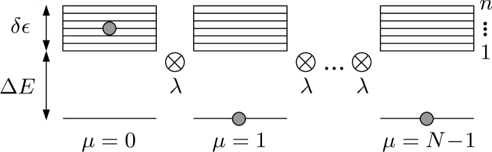
Figure 1: A chain of $N$ identical, weakly coupled subunits which feature a non-degenerate ground state, an energy gap $\Delta E$ and an energy band $\delta\epsilon$ with $n$ equidistant states. The dots indicate excitation probabilities and are supposed to visualize a state from the investigated “single-excitation space”.

In the present Section we firstly consider a model which is “designed” for the application of our method, since it perfectly fulfills almost all properties which have been assumed in the previous Secs. 3-5. The projection onto local densities and second order TCL remarkably allow for a complete characterization of all available types of transport and their dependence on the considered length scale, too.

According to Fig. 1, the model is a chain of $N$ identical subunits which are assumed to feature a non-degenerate ground state, a large energy gap $\Delta E$ and a comparatively narrow energy band $\delta\epsilon$ with $n$ equidistant states. In the following we focus on the “single-excitation subspace”, that is, only one subunit is excited to its band, while all other subunits are in their ground states. Consequently, the local Hamiltonian is given by (2) with $\mu$-independent coefficients $h^{i}=i\,\delta\epsilon/n+\Delta E$.

The next-neighbor interaction (3) is also supposed to be identical for all adjacent subunits. In particular the $\mu$-independent coefficients $v^{i,j}$ form a normalized matrix whose elements are chosen at random from a Gaussian distribution with zero mean. But we do not intend to apply random matrix theory or discuss quantum chaos. For our purposes the crucial point is the fact that matrices of this kind satisfy the van Hove property, see Sec. 4.

However, following the ideas of quantum chaos, we expect that each sufficiently complex one-particle system will take on a form which is similar to our model, once it is partitioned into local subunits and those subunits are diagonalized. The local interactions will effectively be random (Gaussian orthogonal/unitary ensemble) and the local spectra will be more or less equidistant (Wigner level statistics). The influence of the spectral details is discussed below.

Our system may be viewed as a simplified model for, e. g., a chain of coupled atoms, molecules, quantum dots, etc. In this case the hopping of the excitation from one subunit to another corresponds to transport of energy, especially if $\Delta E\gg\delta\epsilon$. This system may also be viewed as a tight-binding model for particles on a lattice. In this case the hopping corresponds to transport of particles. There are $n$ “orbitals” per lattice site but apparently no particle-particle interaction in the sense of the Hubbard model. Although the $v^{i,j}$ are random, these are systems without disorder in the sense of, say, Anderson anderson1958 , since the $v^{i,j}$ are independent from $\mu$. For some literature on this class of systems, see Refs. michel2005 ; gemmer2006 ; steinigeweg2006-2 ; steinigeweg2007-1 ; kadiroglu2007 . Remarkably, a very similar model has been used in Ref. weaver2006 in order to investigate the flow of wave energy in reverberation room acoustics.

In the context of this model we are mainly interested in the probability $p_{\mu}(t)$ for finding an excitation of the $\mu$th subunit to its band, while all other subunits are in their ground state. This quantity is described by (4) with $p^{i}=1/\sqrt{n}$. Because the model is translational invariant and the overall conservation of probability is naturally provided, the projection onto these local quantities and TCL2 immediately leads to (20), that is, the relaxation of $p_{q}(t)$ with the standard rate $-W\,R(t)$. The underlying correlation function $C(\tau)$ reads

$$C(\tau)=\frac{2}{n}\sum_{i,j=0}^{n-1}|v^{i,j}|^{2}\,\cos\!\Big{[}\,\frac{\delta\epsilon\,(i-j)\,\tau}{n}\,\Big{]}\,.$$ (42)

Of course, $C(\tau)$ depends on the concrete realization of the random coefficients $v^{i,j}$. But, due to the law of large numbers, the crucial features are nevertheless the same for the overwhelming majority of all realizations, at least as long as $\sqrt{n}\gg 1$. And in fact, $C(\tau)$ typically assumes the form in Fig. 2. It decays like a standard correlation function on a time scale in the order of $\tau_{C}=1/\delta\epsilon$. The area under this initial peak is approximately given by $R=2\pi\,n/\delta\epsilon$. However, because the local bands possess an equidistant level spacing, $C(\tau)$ is a strictly periodic function with the period $T=2\pi\,n/\delta\varepsilon$, unlike standard correlation functions. As a consequence its time integral $R(t)$ nearly represents a step function, see Fig. 2. A non-equidistant level spacing will certainly “smooth” these steps and change their width, height and distance as well. But we expect that the tendency of an increasing rate $R(t)$ will nevertheless remain.

Figure 2: Sketch of the correlation function $C(\tau)$ [dashed line] and its integral $R(t)$ [continuous line]: $C(\tau)$ features complete revivals at multiples of $T$ such that $R(t)$ has a step-like form. This sketch indeed reflects the numerical results for $C(\tau)$ and $R(t)$ but highlights the relevant time scales for clearness.

Along the lines of Sec. 3, for $\tau_{C}<t<T$ diffusive behavior with a diffusion constant $D=\lambda^{2}\,R$ is to be expected, cf. (21). And indeed, for density profiles $p_{q}(t)$ which decay on such an intermediate time scale we find an excellent agreement between (21) and the numerical solution of the full time-dependent Schrödinger equation (which is obtained by incorporating Bloch’s theorem and exactly diagonalizing the Hamiltonian within decoupled subspaces). In Fig. 3 a “typical” example is shown for a single realization of the random numbers $v^{i,j}$.

Figure 3: Time evolution of a mode $p_{\pi}(t)$ which decays on an intermediate time scale $\tau_{C}<t<T$. Numerics (crosses) shows an exponential decay which indicates diffusive behavior and is in accord with the theoretical prediction (continuous line). Parameters: $N=120$, $n=500$, $\delta\epsilon=0.5$, $\lambda=0.0005$.

However, until now the above picture is not complete for two reasons. The first reason is that $p_{q}(t)$ may decay on a time scale that is long compared to $T$. According to (20), this will happen, if $2\,(1-\cos q)\,\lambda^{2}R\,T\gg 1$ is violated. If we approximate $2\,(1-\cos q)\approx q^{2}=4\pi^{2}/\,l^{2}$ for rather small $q$ (large $l$), we obtain the condition

$$\left(\frac{4\pi^{2}\,n\,\lambda}{l\,\delta\epsilon}\right)^{2}\gg 1\,.$$ (43)

If this condition is satisfied for the largest possible $l$, i. e., for $l=N$, the system exhibits diffusive behavior for all modes. If, however, the system is large enough to allow for some $l$ that violates condition (43), diffusive behavior breaks down in the long-wavelength limit. This result is again backed up by numerics, see Fig. 4.

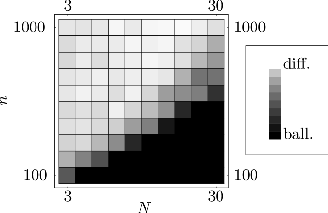
Figure 4: Deviations of the time evolution of Fourier modes $p_{q}(t)$ with $q=2\pi/N$, the longest wavelength, from a purely exponential decay for different model parameters $N$ and $n$. These deviations are based on a measure used in steinigeweg2006-2 and are in accord with the claim that diffusive transport behavior is restricted to the regime defined by condition (43). Other model parameters: $\delta\epsilon=0.5$, $\lambda=0.0005$.

Towards what transport type does the system deviate from diffusive, if condition (43) is violated? As already mentioned above, we have to consider time scales $t\gg T$ in this regime. We may thus approximate $R(t)\approx 2\,R\,t/T$, see Fig. 2. Plugging $D(t)=2\,\lambda^{2}R\,t/T$ into (6) leads to a spatial variance $\sigma^{2}(t)=2\,\lambda^{2}R\,t^{2}/T$, clearly indicating a transition towards ballistic transport. The validity of our approach is again backed up by numerics: In the ballistic regime a Gaussian decay of $p_{q}(t)$ is to be expected, see Fig. 5a.

Figure 5: (a) Evolution of a mode $p_{\pi/60}(t)$ which decays on a time scale $t\gg T$, parameters: $N=120$, $n=500$, $\delta\epsilon=0.5$, $\lambda=0.0005$. (b) Evolution of a mode $p_{\pi}(t)$ which decays on a time scale $t\ll\tau_{C}$, parameters: $N=120$, $n=500$, $\delta\epsilon=0.5$, $\lambda=0.004$. In both cases numerics (crosses) shows a Gaussian decay which indicates ballistic behavior and is in accord with the theoretical predictions (continuous lines).

In a second case transport may be non-diffusive, if the $p_{q}(t)$ decay on a time scale that is short compared to $\tau_{C}$. This will happen, if $2\,(1-\cos q)\,\lambda^{2}R\,\tau_{C}\ll 1$ is violated. If we use the approximation $2\,(1-\cos q)\approx 4$ for the largest possible $q$ (smallest possible $l$), the above inequality may be written as

$$\frac{8\pi\,n\,\lambda^{2}}{\delta\epsilon^{2}}\ll 1\,.$$ (44)

If this inequality is violated, diffusive behavior breaks down in the limit of short-wavelength modes. Moreover, if the second order still yields reasonable results for not too large $\lambda$, we expect a linearly increasing rate $R(t)$ and thus a Gaussian decay, that is, according to the above reasoning, ballistic transport. For increasing wavelength, however, the corresponding inequality will eventually be satisfied, hence allowing for diffusive behavior. Also these conclusions are in accord with numerics, see Fig. 5b.

Relationship to Standard Solid State Theory

Figure 6: Upper section of the $E_{k}$-vs.-$k$ diagram for $N=\infty$ (continuous lines) and $N=10$ (dots). In the limit of small $N$ the band structure of distinct smooth lines apparently breaks down towards a disconnected set of points. Other parameters: $n=500$, $\delta\epsilon=0.5$, $\lambda=0.0005$.

Standard solid state theory always predicts ballistic transport for a translational invariant model without particle-particle interactions. Nevertheless, in the limit of many bands (many orbitals per site) and few sites (few $k$-values) two features may occur: Firstly, the band structure in $k$-space becomes a disconnected set of points rather than the usual set of distinct smooth lines, see Fig. 6. It is therefore impossible to extract velocities by taking derivatives of dispersion relations. And secondly, the eigenstates of the current operator no longer coincide with the Bloch eigenstates of the Hamiltonian such that the current becomes a non-conserved quantity, even in the absence of impurity scattering. It is straightforward manner to check that both features occur in the regime where condition (43) is fulfilled. This is the regime where standard solid state theory breaks down due to the fact that the system is too “small”.

Validity of the TCL Approach and Failure of the NZ Technique

Lowest order TCL suggests the emergence of ballistic transport, if either condition (43) or (44) is violated, e. g., if the coupling strength $\lambda$ is sufficiently weak or strong, respectively. Although the agreement of these predictions with numerics surely is evident, it is desirable to support them by an independent analytical calculation, too. Such calculations are indeed possible in the limit of $\lambda\rightarrow 0$ and $\lambda\rightarrow\infty$, since then first order perturbation theory can be invoked: $\lambda\,\hat{V}$ is a small perturbation to $\hat{H}_{0}$ in the first case and vice versa in the second case. In both limits a localized initial state $\psi(0)=|\mu,i\rangle$ eventually leads to a variance $\sigma^{2}(t)\propto t^{2}$ in the limit $N\rightarrow\infty$. The corresponding proof essentially requires the use of Bessel functions and their properties, see Appendix A for details.

However, in a sense the agreement of the numerical simulations with the TCL2 result is really surprising: The fact that the correlation function $C(\tau)$ features full revivals at multiples of $T$ points towards strong memory effects, cf. Fig. 2. It appears to be a widespread belief that long memory times have to be treated by means of the NZ projection operator technique. Whereas the solutions of NZ2 and TCL2 are almost identical for $\tau_{R}<T$ in the diffusive regime, for $\tau_{R}\gg T$ in the deep ballistic regime the NZ2 equation contrary predicts a purely oscillating behavior of the corresponding density profiles $p_{q}(t)$. But such a behavior obviously contradicts the observed Gaussian decay in Fig. 5 and consequently demonstrates the failure of NZ2 in the description of the long-time dynamics.

Figure 7: Ratio $f(t)$ of fourth to second order contribution at $t=\tau_{R}$ (“best case” approximation). The fact that $f(\tau_{R})\sim 1$ is already reached for rather small $\tau_{R}\sim T$ seems to indicate the breakdown of the TCL2 prediction for ballistic behavior on large length scales. Parameters: $n=500$, $\delta\epsilon=0.5$.

Unfortunately, for this model the unrestricted validity of lowest order TCL cannot be prognosticated by the ideas of Secs. 4 and 5. According to Fig. 7, at $\tau_{R}\sim T$ the fourth order takes on the same order of magnitude as the second order. This finding wrongly indicates the breakdown of the TCL2 prediction for $\tau_{R}\gg T$. One is apparently concerned with a situation where higher order contributions are not individually small but otherwise compensate each other to approximately zero. In such a situation a large but finite fourth order term alone is not suitable as an “alarm” criterion. Note that for this model the fourth order term does not increase arbitrarily and converges to a finite value, see Fig. 7. This will not be the case in the following Sec. 6.2.

6.2 Anderson Model

Since it had been suggested by P. W. Anderson, the Anderson model served as a paradigm for transport in disordered systems anderson1958 ; abouchacra1973 ; lee1985 ; kramer1993 ; erdos2007 ; schwartz2007 . In its probably simplest form the Hamiltonian may be written as

$$\hat{H}=\sum_{\bf r}\epsilon_{\bf r}\,\hat{a}^{\dagger}_{\bf r}\,\hat{a}_{\bf r}+\sum_{\text{NN}}\hat{a}^{\dagger}_{\bf r}\,\hat{a}_{\bf r^{\prime}}\,,$$ (45)

where the $\hat{a}_{\bf r}$, $\hat{a}^{\dagger}_{\bf r}$ are the usual annihilation, respectively creation operators; $\bf r$ labels the sites of a $d$-dimensional lattice; and NN indicates a sum over nearest neighbors. The $\epsilon_{\bf r}$ are independent random numbers, e. g., Gaussian distributed numbers with mean $\langle\epsilon_{\bf r}\rangle=0$ and variance $\langle\epsilon_{\bf r}\,\epsilon_{\bf r^{\prime}}\rangle=\delta_{{\bf r},{\bf r}^{\prime}}\,\sigma^{2}$. Thus, the first sum in (45) describes a random on-site potential and hence disorder.

It is well known that in the presence of disorder, $\sigma\neq 0$, the eigenstates of the Hamiltonian (45) are no longer given by Bloch functions: The eigenstates are not necessarily extended over the whole lattice and can become localized in configuration space, i. e., the envelope of a wavefunction decays exponentially on a finite localization length.

This phenomenon and its impact on transport have intensively been studied for the Anderson model anderson1958 ; abouchacra1973 ; lee1985 ; kramer1993 . For the lower dimensional cases, $d=1$ and $d=2$, it is commonly assumed that all eigenstates feature finite localization lengths for arbitrary (non-zero) values of $\sigma$. Consequently, in the thermodynamic limit, i. e., with respect to the infinite length scale, an insulator is to be expected, see Ref. lee1985 ; kramer1993 . Of particular interest is the $3$-dimensional case, of course. Here, the mobility edge arranges spatially localized and extended wavefunctions into separated regimes in energy space. When the amount of disorder is increased, the mobility edge goes above the Fermi level and a metal-to-insulator transition is induced at zero temperature lee1985 ; kramer1993 , still on the infinite length scale. When $\sigma$ is further increased, above some critical disorder $\sigma_{C}$, all eigenstates become localized and an insulator is to be expected for $T>0$ also. ($\sigma_{C}=W_{C}/\sqrt{12}\approx 6$, where $W_{C}$ is the critical “width” of the Gaussian distribution kramer1993 .)

However, with respect to finite length scales the following transport types are generally expected: (i.) ballistic on a scale below some, say, mean free path; (ii.) possibly diffusive on a scale above this mean free path but below the localization length; and (iii.) insulating on a scale above the localization length.

In the present Section, other than most of the pertinent literature, we do not focus on the mere existence of a finite localization length. Instead we rather concentrate on the size of the intermediate regime and the dynamics within. We especially demonstrate that there exists a length scale regime in which the dynamics is indeed diffusive and characterized by an energy-independent diffusion constant. In principle, this regime could be very large for long localization lengths. But the results in this Section indicate that it is not. Investigations in this direction (but not for $d=3$) are also performed in Refs. schwartz2007 ; lherbier2008 .

Our approach is still based on the form of the TCL technique which has been established in Secs. 3 - 5. In this form the TCL method is restricted to the limit of infinite temperature. This limitation implies that energy dependences are not resolved, i. e., our results are to be interpreted as results for an overall behavior of all energy subspaces. Thus, the regime in which TCL2 holds is characterized by the fact that the dynamics within is diffusive at all energies with a single diffusion constant.

In principle the formalism is also applicable in the case of finite temperatures, but solely in the limit of weak coupling strengths. In this limit the energy subspaces of the full system are directly known from the spectra of the local subunits. The contributions of the initial condition $p_{q}(0)$ to energy subspaces can therefore be weighted with a Boltzmann factor and may be treated separately from each other. But for strong interactions, as it is the typical case for the Anderson model, energy subspaces are simply not extractable from the uncoupled system and merely the case of infinite temperature is accessible.

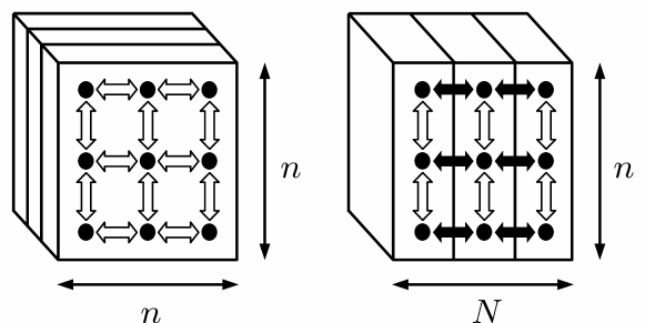
Figure 8: A $3$-dimensional lattice which consists of $N$ layers with $n\times n$ sites each. Only next-neighbor hoppings are taken into account. Constants for intra-layer hoppings are set to $1$ (white arrows), inter-layer hoppings are specified by another constant $\lambda$ (black arrows).

As shown in Fig. 8, we consider a $3$-dimensional (cubic) lattice consisting of $N$ layers with $n\times n$ sites each. For technical reasons we use a Hamiltonian which is almost identical to (45) with a single exception: All those terms corresponding to hoppings between layers are multiplied by some constant $\lambda$. However, for $\lambda=1$ the Hamiltonian reduces to the standard Anderson Hamiltonian (45).

A “coarse-grained” description in terms of subunits is established now: At first we take all those terms of the Hamiltonian which only contain the sites of the $\mu$th layer in order to form the local Hamiltonian $h_{\mu}$ of the subunit $\mu$. Thereafter all those terms which contain the sites of neighboring layers $\mu$ and $\mu+1$ are selected in order to form the interaction $\lambda\,\hat{v}_{\mu,\mu+1}$ between adjacent subunits $\mu$ and $\mu+1$. Then the total Hamiltonian may be also written in the form of (1) as $\hat{H}=\hat{H}_{0}+\lambda\,\hat{V}$. Note that in this form the additional parameter $\lambda$ allows for the independent adjustment of the interaction strength. The eigenbasis of $\hat{H}_{0}$ may be found from the diagonalization of disconnected layers.

By $\hat{p}_{\mu}$ we denote the particle number operator of the $\mu$th subunit, i. e., the sum of $\hat{a}^{\dagger}_{\bf r}\,\hat{a}_{\bf r}$ over all ${\bf r}$ of the $\mu$th layer. Since the overall number of particles is conserved, $[\,\sum_{\mu}\hat{p}_{\mu},\hat{H}\,]=0$, and no particle-particle interactions are taken into account, we choose to restrict the analysis to the one-particle subspace. We may therefore implement $\hat{p}_{\mu}$ by (4) with $p^{i}=1/n$. The corresponding expectation value $p_{\mu}(t)$ is the probability for locating the particle somewhere within the $\mu$th subunit. The consideration of these “coarse-grained” probabilities corresponds to the investigation of transport along the direction which is perpendicular to the layers, cf. Fig. 8. Instead of simply characterizing whether or not there is transport at all, we analyze the full dynamics of the $p_{\mu}(t)$.

According to Sec. 3, the application of our method requires that two conditions are fulfilled: (i.) the overall conservation of probability which is naturally provided; and (ii.) the “average” translational invariance in terms of a correlation function

$$C(\tau)=\frac{1}{n^{2}}\,\text{Tr}\{\,\hat{v}_{\mu,\mu+1}(t)\,\hat{v}_{\mu,\mu+1}(t_{1})\,\}$$ (46)

which depends only negligibly on the concrete choice of the layer number $\mu$ (during some relevant time scale). Simple numerics indicates that this assumption is well fulfilled (for the values of $\sigma$ which are discussed here), once the layer sizes exceed ca. $30\times 30$. Exploiting this assumption immediately leads to the TCL2 prediction (20), namely, the relaxation of Fourier modes $p_{q}(t)$ with the standard rate $-W\,R(t)$. The underlying correlation function is the above $C(\tau)$, of course.

Direct numerics shows that $C(\tau)$ again looks like a standard correlation function. We thus retain the former notation of $\tau_{C}$ as the correlation time and $R$ as the area under the initial peak of $C(\tau)$. The numerical results also indicate that neither $\tau_{C}$ nor $R$ depend substantially on $n$ (at least for $n>30$). Consequently, both $\tau_{C}$ and $R$ are essentially functions of $\sigma$.

Figure 9: Time evolution of modes $p_{q}(t)$ with $q=\pi$ (shortest wavelength) and $q=2\pi/N$ (longest wavelength) for $\lambda=0.24$ (circles) and $\lambda=0.08$ (squares). Remaining model parameters: $n=30$, $\sigma=1$, and $N=10$. Symbols are obtained numerically from exact diagonalization, whereas all curves correspond to the theoretical TCL2 predictions. Additional data from a 4th order Suzuki-Trotter integrator is shown in (b) for the case of $\lambda=1$ and $N=42$ (triangles). Note that the curves in (b) and (c) are identical, since the factor $W$ is the same, see text for details. Further note that the transition from (a) towards (d) is to be expected for larger $N$ with a single choice of $\lambda$. For evidence in that direction, see Fig. 10.

Figure 10: Numerical illustration of the transition in Fig. 9 for a fixed $\lambda$. Model parameters: $n=20$, $\sigma=1$, $N=26$, and $\lambda=0.24$. Smaller layer sizes ($n=20$) are chosen to allow for exact diagonalization of a system with a larger number of layers ($N=26$). Note that theoretical curves are not indicated, since for $n=20$ the “average” translational invariance is not well fulfilled yet.

According to all above findings and the reasoning in Sec. 3, for $t>t_{C}$ diffusive behavior with a diffusion constant $D=\lambda^{2}\,R$ is to be expected in TCL2, cf. (21). Due to the independence of $R$ from both $n$ and $N$, the pertinent diffusion constant for arbitrarily large systems may be quantitatively inferred from the diagonalization of a finite, e. g., “$30\times 30$ layer”.

In order to check the above theory, we exemplarily present some results here. For $n=30$ and, e. g., $\sigma=1$ we numerically find $\tau_{C}\approx 10$ and $R\approx 2.9$. Thus, additionally choosing $\lambda=0.24$ and considering the longest wavelength in a $N=10$ system ($q=\pi/\,5$), we obtain $W\,R\approx 0.064$. This corresponds to a ratio $\tau_{R}/\tau_{C}\approx 1.6$ and hence $\tau_{R}>\tau_{C}$ which justifies the replacement of (20) by (21). And indeed, for the dynamics of $p_{q}(t)$ we get an excellent agreement of the theoretical prediction based on (21) with the numerical solution of the full time-dependent Schrödinger equation, see Fig. 9b. Note that this solution is obtained by the use of exact diagonalization. Naturally interesting is the “isotropic” case of $\lambda=1$. Keeping $\sigma=1$, one has to go to the longest wavelength in a $N=42$ system in order to keep the $W$ of the former example unchanged. If our theory applies, the decay curve should be the same. This indeed turns out to hold, see Fig. 9b. Note that the integration in this case already requires approximative numerical integrators like, e. g., Suzuki-Trotter decompositions steinigeweg2006-1 . A numerical integration of systems with larger $N$ rapidly becomes unfeasible but an analysis based on (21) may always be performed.

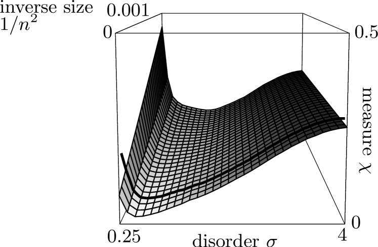
Figure 11: Numerical results for the measure $\chi$ with respect to the disorder $\sigma$ and the inverse layer size $1/n^{2}$ (“best case approximation”). $\chi$ detects the corridor of length scales where the overall behavior of all energy regimes is diffusive. For those values of $\chi$ which are in the order of $1/4$ the corridor does not exist. But for those values of $\chi$ which are closer to $0$, the corridor opens and diffusive behavior is present in all energy regimes with a single diffusion constant. The smaller $\chi$, the larger is this corridor of diffusive length scales. An absolute minimum $\chi_{\text{min}}\approx 0.02$ is found at $\sigma\approx 0.5$ in the limit of $n\rightarrow\infty$. Note that only $10\%$ of the whole area is extrapolated (the area in front of the thick line).

So far, we have characterized the dynamics of the diffusive regime. We now turn towards an investigation of its size. To this end we consider the measure $\chi$ which has been introduced in Secs. 4 and 5. Recall that this measure yields $l_{\text{min}}/l_{\text{max}}\approx 2\,\sqrt{\chi}$, cf. (37).

$l_{\text{min}}$ is the length scale where diffusive dynamics breaks down due to the fact that the corresponding $p_{q}(t)$ decays on a comparatively short time scale $\tau_{R}\approx\tau_{C}$. In complete analogy to the former model, this transition is still correctly described by TCL2: $R(t)$ is not approximately constant but linearly increases during the relaxation period. This strongly indicates a transition towards ballistic behavior, see Fig. 9a.

Contrary, $l_{\text{max}}$ is the length scale where diffusive dynamics breaks down, because the corresponding $p_{q}(t)$ decays on a long time scale $\tau_{R}$ at which the additional contribution $S(t)$ becomes non-negligible, cf. (30). Since the interaction perfectly fulfills the van Hove structure, $S(t)$ essentially reflects fourth order effects which account for, e. g., insulating behavior, cf. Fig. 9d. [Note that all our data available from exact diagonalization is in accord with a description based on (30). Note further that $S(t)$, other than $R(t)$, scales significantly with $n$. This eventually gives rise to the $n$-dependence in Fig. 11.]

As shown in Fig. 11, for each layer size $n$ there is some disorder which minimizes $\chi$ and hence “optimizes” the diffusive regime. However, for $n=30$ (back of Fig. 11) we find $\sqrt{\chi_{\text{min}}}\approx 1/3$ at this optimum disorder, indicating about one diffusive wavelength. Exactly those respective wavelengths have been chosen for the examples in Figs. 9b,c but not in Fig. 9d. For all $\sigma$ and up to $n=100$ (which is about the limit for our numerics) $\chi$ clearly appears to be of the form $\chi(\sigma,n)=A(\sigma)/n^{2}+B(\sigma)$. Extrapolating this $1/n^{2}$-behavior yields a suggestion for the infinite model $n=\infty$ (front of Fig. 11). According to this suggestion, we find $\sqrt{\chi_{\text{min}}}\approx 1/7$, again at optimum disorder. This indicates a rather small regime of diffusive wavelengths, even for the infinite system.

We finally recall that these findings apply at infinite temperature, i. e., the small diffusive regime is characterized by the fact that the dynamics within is diffusive at all energies with a single diffusion constant. The absence of diffusive dynamics in the limit of strong disorder apparently agrees with the common expectation that diffusion at each energy stops completely, once $\sigma$ reaches a value larger than $\sigma_{C}\approx 6$ and all eigenstates become localized lee1985 ; kramer1993 . Down to intermediate amounts of disorder the localization phenomenon certainly plays a crucial role for the smallness of the diffusive regime. In the limit of weak disorder, however, localization appears to be less important, especially since only few eigenstates in the outer tails of the density of states are localized, while the overwhelming majority is extended. In that limit the smallness of the regime in which TCL2 holds may result from the fact that diffusive dynamics is present at each energy but with a energy-dependent diffusion constant, cf. kramer1993 . Then the overall behavior of all energy subspaces is a multi-exponential decay and not diffusive, of course. On that account it appears plausible that the diffusive regime becomes much larger, if only a certain subspace of energy is considered.

7 Summary and Conclusion

In this work the TCL projection operator technique has been applied to quantum transport in modular systems. In particular, the projection onto local densities and the lowest order contribution of the TCL expansion have been used as a strategy for the analysis of transport and its length scale dependence. Furthermore, an estimation for the range of validity of the lowest order prediction has been derived by means of an extension of the standard projection that includes additional relevant degrees of freedom. This estimation is especially suited for interaction types with van Hove structure and also provides an interpretation in the context of length scales.

As a first application a single-particle model has been investigated which has randomly structured interactions but nevertheless is translational invariant. For this model a full characterization of all types of transport behavior has been obtained. Remarkably, purely diffusive behavior has been demonstrated to occur on an intermediate length scale which is bounded by completely ballistic regimes in the limit of short and long length scales.

The next step in the context of single-particle models has been performed by the introduction of disorder. The 3D Anderson model has been shown to exhibit fully diffusive dynamics on an intermediate length scale between mean free path and localization length. But it has also been demonstrated that the diffusive regime is extremely small, at least in the considered limit of high temperatures.

Naturally, a further important step is given by the application of the theory to interacting many-particle systems with or without disorder. In fact, there are already preliminary results for a “many-particle” model which is translational invariant, has randomly structured interactions but does not allow for any single-particle restriction. This model has been discussed only briefly steinigeweg2006-2 ; gemmer2006 and basically seems to show the same dynamical behavior as its single-particle analog, that is, diffusive dynamics on intermediate length scales breaks down towards ballistic transport in the limit of large length scales. The main problem for this system arises from the fact that a direct comparison of the second order prediction with the numerical solution of the time-dependent Schrödinger equation is not feasible for sufficiently large systems. Consequently, an appropriate estimate for the validity range of second-order TCL of the type derived in this paper is indispensable.

Appendix A Analytically Solvable Limit Cases

The results of Sec. 6.1 strongly suggest the occurrence of ballistic transport in the two limit cases (43) and (44) of weak and strong coupling strength $\lambda$. Since these results depend on the applicability of the TCL2 method, it would be desirable to support them by independent analytical calculations. Such calculations are possible in the two limit cases $\lambda\rightarrow 0$ and $\lambda\rightarrow\infty$, since then first order perturbation theory can be invoked. Moreover, we will restrict ourselves to the case where the Hamiltonian given by Eqs. (1)-(3) is translational invariant and the next-neighbor interaction matrix (3) is symmetric, i. e., we will assume

$$h_{\mu}^{i}=h_{0}^{i}\equiv h^{i}\;,$$ (47)

$$v_{\mu,\mu+1}^{i,j}=v_{0,1}^{i,j}=v_{0,1}^{j,i}\equiv v^{i,j}\;.$$ (48)

In these calculations various sums over $\mu=0,1,\ldots,N-1$ occur, which will be most conveniently approximated by integrals. This approximation is exact in the limit $N\rightarrow\infty$. The variance (6) will be considered with local “excitation densities” (4) using $p_{\mu}^{i}=1$.
Let us assume that the symmetric next-neighbor interaction matrix $v$ has been diagonalized:

$$\sum_{j=0}^{n-1}v^{i,j}\,S_{k}^{j}=s_{k}\,S_{k}^{i}$$ (49)

We will consider the time evolution of an initially localized excitation, i. e., a solution

$$\varphi(t)=\sum_{\mu,i}\varphi_{\mu}^{i}(t)\,|\mu,i\rangle$$ (50)

of the Schrödinger equation with the initial value $\varphi_{\mu}^{i}(0)=\delta_{\mu,0}\,\delta_{i,0}$.

A.0.1 The case $\lambda\rightarrow 0$

In the limit $\lambda\rightarrow 0$ and $N\rightarrow\infty$ we obtain

$$\left|\varphi_{\mu}^{i}(t)\right|^{2}\sim\delta_{i,0}\left|J_{|\mu|}\!\left(2\,\lambda\,v^{0,0}\,t\right)\right|^{2}\;,$$ (51)

where $J_{|\mu|}$ denotes the $|\mu|$-th Bessel function, and as a consequence

$$\sigma^{2}(t)=\sum_{\mu,i}\mu^{2}\,\left|\varphi_{\mu}^{i}(t)\right|^{2}\sim 2\,\lambda^{2}\,v^{0,0}\,t^{2}\,,$$ (52)

indicating ballistic transport.

A.0.2 The case $\lambda\rightarrow\infty$

Upon rescaling the Hamiltonian (1) in the form

$$\hat{H}=\frac{1}{\lambda}\,\hat{H_{0}}+\hat{V}$$ (53)

we can again apply first order perturbation theory. This yields eigenvalues of the form

$$E_{k,\mu}=\frac{1}{\lambda}\,E_{k}+2\,s_{k}\cos\frac{2\pi\,\mu}{N}\,,$$ (54)

where

$$E_{k}=\sum_{i}\left|S_{k}^{i}\right|^{2}h^{i}\,.$$ (55)

Consequently,

$$\!\!\!\left|\varphi_{\mu}^{i}(t)\right|^{2}$$

$$\sim \!\!\!\left|\sum_{k}\overline{S_{k}^{0}}\,S_{k}^{i}\,\exp\left(\frac{-\imath\,E_{k}\,t}{\lambda}\right)J_{|\mu|}\!\left(2\,s_{k}\,t\right)\right|^{2}\!.$$ (56)

In order to evaluate the variance (6) we will utilize the following formula, stated without proof,

$$\!\!\!\sum_{m=-\infty}^{\infty}\,m^{2}\,J_{n+m}(s)\,J_{m}(t)$$

$$= \!\!\!\frac{t^{2}}{4}\left[J_{n+2}(s-t)+J_{n-2}(s-t)+2\,J_{n}(s-t)\right]$$

$$+ \!\!\!\frac{t}{2}\left[J_{n+1}(s-t)-J_{n-1}(s-t)\right]$$ (57)

in the special case of $n=0$. We then obtain for the leading term

$$\sigma^{2}(t)\sim 2\,t^{2}\,\sum_{k}\left|S_{k}^{0}\right|^{2}s_{k}^{2}+{\cal O}(t)\;,$$ (58)

again indicating ballistic transport. Numerical tests show that the parabolic approximation (58) is very close for all times.

- (1) S. Nakajima, Progr. Theor. Phys. 20, 948 (1958)
- (2) R. Zwanzig, J. Chem. Phys. 33, 1338 (1960)
- (3) S. Chaturvedi, F. Shibata, Z. Phys. B 35, 297 (1979)
- (4) H. P. Breuer, F. Petruccione, The Theory of Open Quantum Systems (Oxford University Press, Oxford, 2007)
- (5) H. P. Breuer, J. Gemmer, M. Michel, Phys. Rev. E 73, 016139 (2006)
- (6) H. B. Breuer, Phys. Rev. A 75, 022103 (2007)
- (7) R. Steinigeweg, H.-P. Breuer, J. Gemmer, Phys. Rev. Lett. 99, 150601 (2007)
- (8) H. Weimer, M. Michel, J. Gemmer, G. Mahler, Phys. Rev. E 77, 011118 (2008)
- (9) L.-A. Wu, D. Segal, Phys. Rev. E 77, 060101R (2008)
- (10) C. Bartsch, R. Steinigeweg, J. Gemmer, Phys. Rev. E 77, 011119 (2008)
- (11) L. Van Hove, Physica 21, 517 (1954)
- (12) L. Van Hove, Physica 23, 441 (1957)
- (13) M. Michel, G. Mahler, J. Gemmer, Phys. Rev. Lett. 95, 180602 (2005)
- (14) P.W. Anderson, Phys. Rev. 109, 1492 (1958)
- (15) J. Gemmer, R. Steinigeweg, M. Michel, Phys. Rev. B 73, 104302 (2006)
- (16) R. Steinigeweg, J. Gemmer, M. Michel, Europhys. Lett. 75, 406 (2006)
- (17) M. Kadiroḡlu, J. Gemmer, Phys. Rev. B 76, 024306 (2007)
- (18) R. Weaver, Phys. Rev. E 73, 036610 (2006)
- (19) R. Abou-Chacra, D. J. Thouless, P. W. Anderson, J. Phys. C 6, 1734 (1973)
- (20) P. A. Lee, T. V. Ramakrishnan, Rev. Mod. Phys. 57, 287 (1985)
- (21) B. Kramer, A. MacKinnon, Rep. Progr. Phys. 56, 1469 (1993)
- (22) L. Erdős, M. Salmhofer, H.-T. Yau, Annales Henri Poincare 8, 621 (2007)
- (23) T. Schwartz, G. Bartal, S. Fishman, M. Segev, Nature 446, 52 (2007)
- (24) A. Lherbier, B. Biel, Y.-M. Niquet, S. Roche, Phys. Rev. Lett. 100, 036803 (2008)
- (25) R. Steinigeweg, H.-J. Schmidt, Comp. Phys. Comm. 174, 853 (2006)