Disappearance of quasi-fermions in the strongly coupled plasma
from the Schwinger-Dyson equation
with in-medium gauge boson propagator

Abstract

We non-perturbatively study the fermion spectrum in the chiral symmetric phase focusing on the effects of in-medium corrections for gauge boson. The fermion spectrum is derived by solving the Schwinger-Dyson equation (SDE) with ladder approximation on the real time axis. It is shown that the peak of the fermion spectral function is broadened by in-medium effects for gauge boson compared with the peak obtained with the tree gauge boson propagator. The peak becomes much broader as the value of the gauge coupling increases. This broadening is caused by multiple scatterings of fermions and gauge bosons included through the non-perturbative resummation done by the SDE. In particular, the Landau damping of gauge boson propagator plays an important role in the broadening. Our results show no clear peak in the strong coupling region, implying the disappearance of quasi-fermions in the strongly coupled plasma. This indicates that quasi-particle picture may be no longer valid in the strongly coupled QGP.

1 Introduction

In the quark-gluon plasma (QGP) quarks and gluons, existing as elementary degrees of freedom, have different spectra from those for the non-interacting quarks and gluons. In the weak coupling limit ($g\ll 1$), employing the Hard Thermal Loop (HTL) approximation, it is shown[1, 2] that light quarks (such as $u$ and $d$) and gluons have poles with masses proportional to the temperature $T$ and the gauge coupling $g$ but no widths.

Recent experimental studies carried out at RHIC[3], on the other hand, suggests that the QGP near the phase transition is a strongly interacting system. This result seems consistent with the findings of recent studies employing lattice QCD, which show that the lowest charmonium state survives at $T$ higher than the critical temperature ($T_{c}$)[4].

For the thermal mass of quark near $T_{c}$, several analyses show $M_{\rm quark}/T\sim 1$ based on one-loop calculation taking the gluon condensate into account[5], Brueckner-type many-body scheme and data from the heavy quark potential in the lattice QCD[6], Nambu–Jona-Lasinio model[7]. In the work done in Refs. Harada:2007gg and Harada:2008vk, an analysis employing the Schwinger-Dyson equation (SDE) is carried out to show that the thermal mass of fermion in the very strong coupling region saturates at $M_{\rm quark}/T\sim 1$, which is consistent with the result by a quenched lattice QCD with two-pole fitting[10].

It is important to study not only the thermal mass but also the entire spectral function for clarifying the properties of quarks in medium. In Ref. Mannarelli:2005pz, the imaginary part of the quark self-energy is shown to be on the order of the thermal mass. Analyses in Refs. Harada:2007gg and Harada:2008vk show that peaks of the spectral function become broad in the strong coupling region. The SDE used in Ref. Harada:2007gg is solved with the tree gauge boson propagator, which shows the broadening of the peaks with increasing coupling. This is understood from the fact that the probability of gauge boson emission and absorption from a fermion increases rapidly with the coupling.

In the present work, we investigate the effects of medium modified gauge boson on the fermion spectral function. We employ the HTL corrected gauge boson propagator to include the characteristic properties of collective excitations of the gauge boson, i.e. quasi-particle poles and the Landau damping. We will pay special attention to the effect of Landau damping and show that it gives further broadening owing to multiple scatterings with fermions and gauge bosons, resulting no clear peak in the spectral function in the strong coupling region.

The contents of this paper are as follows. In section 2, we introduce the SDE on the real time axis as an iterative equation for the fermion spectral function[9]. In section 3, the fermion spectral function obtained in this way are shown focusing on the effects of medium corrected gauge boson. Section 4 is devoted to a brief summary and discussions. In appendices, we show the phase structure in our frame work, and dependence on the difference of the method for solving the SDE and the gauge fixing condition.

2 The Schwinger-Dyson equation at Finite $T$

The SDE for the fermion propagator ${\mathcal{S}}$ in the imaginary time formalism is expressed as

$${\mathcal{S}}^{-1}(i\omega_{n},\vec{p}) -{\mathcal{S}}_{free}^{-1}(i\omega_{n},\vec{p})=\Sigma(i\omega_{n},\vec{\vec{p}})$$

$$=g^{2}T\sum_{m=-\infty}^{\infty}\int\frac{d^{3}k}{(2\pi)^{3}}\gamma_{\mu}{\mathcal{S}}(i\omega_{m},\vec{k})\gamma_{\nu}{\mathcal{D}^{\mu\nu}}(i\omega_{n}-i\omega_{m},\vec{p}-\vec{k}),$$ (1)

where $\Sigma$ and ${\mathcal{D}}$ are the fermion self-energy and a gauge boson propagator, respectively, and $\omega_{n}=(2n+1)\pi T$ is the Matsubara frequency for the fermion. The SDE was employed to describe the spontaneous chiral symmetry breaking in the strong coupling gauge theories[11, 12, 13, 14, 15, 16]. When the value of the gauge coupling $g$ in Eq. (1) is larger than the critical value $g_{c}$, the chiral symmetry is spontaneously broken at low $T$. When $g$ is smaller than $g_{c}$, on the other hand, the chiral symmetry is not broken even at $T=0$. We summarize the phase structure in appendix A. In the following, we consider only the chiral symmetric phase to investigate the fermion spectrum.

We start with formulating the SDE on the real time axis following Ref. Harada:2008vk. The Matsubara summation in Eq. (1) can be performed by using the spectral representation for fermion and gauge boson propagators as follows:

$$\Sigma(i\omega_{n},\vec{p})= -g^{2}\int\frac{d^{3}k}{(2\pi)^{3}}\int dz\int dz^{\prime}\frac{1}{i\omega_{n}-z-z^{\prime}}\left(1-f(z)+n(z^{\prime})\right)$$

$$\times\left[\gamma_{\mu}\rho_{f}(z,\vec{k})\gamma_{\nu}\rho_{B}^{\mu\nu}(z^{\prime},\vec{p}-\vec{k})\right],$$ (2)

where $f$ ($n$) is the Fermi-Dirac (Bose-Einstein) distribution function, and $\rho_{f}$ and $\rho_{B}^{\mu\nu}$ are the spectral functions for the fermion and the gauge boson introduced as

$${\mathcal{S}}(i\omega_{m},\vec{p}) =-\int dz\frac{\rho_{f}(z,\vec{k})}{i\omega_{m}-z},$$

$${\mathcal{D}}^{\mu\nu}(i\omega_{n}-i\omega_{m},\vec{p}-\vec{k}) =-\int dz\frac{\rho^{\mu\nu}_{B}(z^{\prime},\vec{p}-\vec{k})}{i\omega_{n}-i\omega_{m}-z^{\prime}}.$$ (3)

Then we replace the Matsubara frequency as $i\omega_{n}\rightarrow p_{0}+i\epsilon$ to obtain the retarded fermion self-energy as

$$\Sigma_{R}(p_{0},\vec{p})=-g^{2}\int\frac{d^{3}k}{(2\pi)^{3}}\int dz \int dz^{\prime}\frac{1}{p_{0}+i\epsilon-z-z^{\prime}}\left(1-f(z)+n(z^{\prime})\right)$$

$$\times\left[\gamma_{\mu}\rho_{f}(z,\vec{k})\gamma_{\nu}\rho_{B}^{\mu\nu}(z^{\prime},\vec{p}-\vec{k})\right].$$ (4)

Taking the imaginary parts of both sides, we have

$${\rm Im}\Sigma_{R}(p_{0},\vec{p})=\pi g^{2}\int^{\Lambda}\frac{d^{3}k}{(2\pi)^{3}} \int_{-\Lambda}^{\Lambda}dk_{0}\left(1-f(k_{0})+n(p_{0}-k_{0})\right)$$

$$\times\left[\gamma_{\mu}\rho_{f}(k_{0},\vec{k})\gamma_{\nu}\rho_{B}^{\mu\nu}(p_{0}-k_{0},\vec{p}-\vec{k})\right],$$ (5)

where $\Lambda$ is the ultraviolet cutoff introduced for regularization. Using the dispersion relation, the real part of the retarded fermion self-energy is expressed as

$${\rm Re}\Sigma_{R}(p_{0},\vec{p}) =\frac{1}{\pi}{\rm P}\int_{-\Lambda}^{\Lambda}dp_{0}^{\prime}\frac{{\rm Im}\Sigma_{R}(p_{0}^{\prime},\vec{p})}{p_{0}^{\prime}-p_{0}},$$ (6)

where ${\rm P}$ denotes the principal integral. The full retarded fermion propagator is expressed with the retarded fermion self-energy $\Sigma_{R}(p_{0},\vec{p})$ as

$$iS_{R}(p_{0},\vec{p})=\frac{-1}{\ooalign{\hfil/\hfil\crcr$p$}+\Sigma_{R}}.$$ (9)

The spectral function for full fermion propagator is in turn expressed with the retarded propagator as

$$\rho_{f}(p_{0},p)=\frac{1}{\pi}{\rm Im}\left[iS_{R}(p_{0},\vec{p})\right],$$ (10)

where $p=|\vec{p}|$ and we remark that the fermion spectral function $\rho_{f}$ has spinor structure. Equations (5), (6), (9) and (10) make a closed form for the spectral function of fermion $\rho_{f}$ when the spectral function of gauge boson $\rho_{B}^{\mu\nu}$ is a known function. In the method used in the previous work[8], we computed both real and imaginary parts of fermion propagator. The present formulation has the advantage of reducing the computation task, because we only compute the imaginary part of fermion self-energy from the loop integral, while the real part is computed from the imaginary part using the dispersion relation.

To make Eqs. (5)–(10) a closed form, we choose an appropriate gauge boson propagator for the system. In the present work, to study the effects of collective excitations of gauge boson, we use the HTL corrected gauge boson propagator in the Coulomb gauge. In the previous work[8], we used the Feynman gauge to avoid double pole term. When we take account of the HTL correction to the gauge boson, we encounter the double pole term in the Landau gauge as well as in the Feynman gauge. In the present work, for simplicity of computation, we choose the Coulomb gauge in which there is no double pole term. We will discuss the dependence of the fermion spectrum on the gauge choice in appendix B in the case of tree gauge boson propagator.

The spectral function of the HTL corrected gauge boson in the Coulomb gauge is expressed as

$$\rho_{B}^{\mu\nu}(q_{0},q)=\rho_{T}(q_{0},q)P_{T}^{\mu\nu}+\rho_{L}(q_{0},q)\delta^{\mu 0}\delta^{\nu 0},$$ (11)

where $P_{T}^{\mu\nu}$ is the transverse projection $P_{T}^{00}=P_{T}^{0i}=0$, and $P_{T}^{ij}=\delta^{ij}-q^{i}q^{j}/q^{2}$. $\rho_{T}^{\mu\nu}$ and $\rho_{L}^{\mu\nu}$ are spectral functions for transverse and longitudinal parts of the HTL corrected gauge boson propagator. They are expressed as [2]

$$\rho_{T}(q_{0},q)=Z_{T}(q)[\delta(q_{0}-\omega_{T}(q))-\delta(q_{0}+\omega_{T}(q))]+\beta_{T}(q_{0},q),$$ (12)

$$\rho_{L}(q_{0},q)=Z_{L}(q)[\delta(q_{0}-\omega_{L}(q))-\delta(q_{0}+\omega_{L}(q))]+\beta_{L}(q_{0},q),$$ (13)

where $\omega_{T}(q)$ and $\omega_{L}(q)$ are dispersion relations of the transverse and longitudinal gauge bosons, $\beta_{T}$ and $\beta_{L}$ are continuum parts of spectral functions and $Z_{T}$ and $Z_{L}$ are pole residues. They are expressed as

$$\beta_{T}(q_{0},q)=\frac{m_{g}^{2}x(1-x^{2})\frac{\theta(1-x^{2})}{2}}{\left(q^{2}(x^{2}-1)-m_{g}^{2}\left[x^{2}+\frac{x(1-x)}{2}\ln\left|\frac{x+1}{x-1}\right|\right]\right)^{2}+\frac{\pi^{2}m_{g}^{4}x^{2}(1-x^{2})^{2}}{4}},$$ (14)

$$\beta_{L}(q_{0},q)=\frac{m_{g}^{2}x\theta(1-x^{2})}{\left[q^{2}+2m_{g}^{2}\left(1-\frac{x}{2}\ln\left|\frac{x+1}{x-1}\right|\right)\right]^{2}+\pi^{2}m_{g}^{4}x^{2}},$$ (15)

$$Z_{T}(q)=\frac{\omega_{T}(q)(\omega_{T}^{2}(q)-q^{2})}{3\omega_{p}^{2}\omega_{T}^{2}(q)-(\omega_{T}^{2}(q)-q^{2})},~{}~{}Z_{L}(q)=\frac{\omega_{L}(q)(\omega_{L}^{2}(q)-q^{2})}{q^{2}(q^{2}+2m_{g}^{2}-\omega_{L}^{2}(q))},$$ (16)

where $m_{g}$ is the thermal mass of gauge boson and is related with the plasma frequency $\omega_{p}$ as $\omega_{p}=\sqrt{2/3}m_{g}=\omega_{T,L}(0)$.

It is useful to parameterize the retarded fermion self-energy $\Sigma_{R}$ and the fermion spectral function $\rho_{f}$ as follows:

$$\Sigma_{R} =\Sigma_{R}^{0}\gamma_{0}-\Sigma_{R}^{\rm v}\frac{\vec{p}}{p}\cdot\vec{\gamma},$$

$$\rho_{f} =\frac{1}{\pi}{\rm Im}~{}iS_{R}(p_{0},p)=\frac{1}{2}\left(\gamma_{0}-\frac{{\vec{p}}}{p}\cdot\vec{\gamma}\right)\rho_{+}+\frac{1}{2}\left(\gamma_{0}+\frac{{\vec{p}}}{p}\cdot\vec{\gamma}\right)\rho_{-},$$ (17)

in which $\rho_{+}$ ($\rho_{-}$) is the fermion spectral function for (anti-) fermion sector. Substituting Eqs. (11) and (17) into Eq. (5) and making suitable projections, the energy part ($\Sigma_{R}^{0}$) and the vector part ($\Sigma_{R}^{\rm v}$) of the retarded self-energy become

$${\rm Im}\Sigma_{R}^{0}(p_{0},\vec{p}) =\pi g^{2}\int^{\Lambda}\frac{d^{3}k}{(2\pi)^{3}}\int^{\Lambda}dk_{0}\left(1-f(k_{0})+n(q_{0})\right)\frac{\rho_{+}(k_{0},\vec{k})+\rho_{-}(k_{0},\vec{k})}{2}$$

$$\hskip 10.00002pt\times\left[2\rho_{T}(q_{0},q)+\rho_{L}(q_{0},q)\right],$$ (18)

$${\rm Im}\Sigma_{R}^{\rm v}(p_{0},\vec{p}) =\pi g^{2}\int^{\Lambda}\frac{d^{3}k}{(2\pi)^{3}}\int^{\Lambda}dk_{0}\left(1-f(k_{0})+n(q_{0})\right)\frac{\rho_{+}(k_{0},\vec{k})-\rho_{-}(k_{0},\vec{k})}{2}$$

$$\hskip 10.00002pt\times\left[2\rho_{T}(q,q)\frac{-pk+(p^{2}+k^{2})\cos\theta-pk\cos^{2}\theta}{q^{2}}-\rho_{L}(q_{0},q)~{}\cos\theta\right],$$ (19)

where $q_{0}=p_{0}-k_{0}$ and $q=|\vec{p}-\vec{k}|$. Equations (18), (19), (6), (9) and (17) make a set of iterative equations for the spectral functions $\rho_{\pm}$ in a closed form.

3 Numerical Results

In the following, we fix the cutoff $\Lambda$ as $\Lambda/T=5$, and we show only $\rho_{+}$ noting the relation $\rho_{-}(p_{0},p)=\rho_{+}(-p_{0},p)$ obtained from the charge conjugation invariance.

In Fig. 1, we plot the fermion spectral function $\rho_{+}$ for $g=1,~{}2$ and $3$, where three upper panels represent the spectral functions of fermion interacting with the tree gauge boson and three lower panels represent those of fermion interacting with the HTL corrected gauge boson with $m_{g}=gT/\sqrt{6}$. In the upper panels, we see that $\rho_{+}$ has two peaks in the low momentum region, one in the positive energy region corresponding to the normal quasi-fermion, and another in the negative energy region corresponding to the anti-plasmino. Two peaks become broad as the coupling increases. In the higher momentum region, fermion spectrum approaches the one of free fermion. These results are consistent with those in the previous work [8]. Comparing fermion spectra in the lower panels with those in the upper panels, we find that two peaks in the lower panels are broader than those in the upper panels, i.e. two peaks become broader by the effects of the thermal correction to the gauge boson in medium. In lower panels, two peaks become broader as the coupling increases as in the upper panels. At $g=2$, although we can see clear two peaks in the upper panel, two peaks in the lower panel are very broad, and the quasi-particle picture seems no longer valid. At $g=3$ in lower panel there is no clear peak, which implies the disappearance of quasi-fermions.

Figure 1: The fermion spectral function $\rho_{+}$ in the Coulomb gauge. Fermion spectra in the upper panels are employing the tree gauge boson and those in the lower panels are employing the HTL corrected gauge boson with $m_{g}/T=g/\sqrt{6}$. When we go from the left panels to the right panels, the coupling becomes stronger in both upper and lower panels: $g=1$ (left panels), $g=2$ (middle panels) and $g=3$ (right panels). The figures are clipped at $\rho_{+}T=2$.

The broadening of the peak with increasing coupling, as we stated in the previous work[8], can be understood as the increasing probability of the gauge boson emission and absorption from a fermion. Because the SDE contains the effects of multiple scatterings with gauge bosons through the self-consistency condition, the peak obtained by the SDE is broader than the one obtained by the one-loop approximation (see Ref. Harada:2007gg).

The difference between the HTL corrected gauge boson and tree gauge boson lies in the difference of the value of $m_{g}/T$: The HTL corrected gauge boson becomes tree gauge boson when $m_{g}/T=0$ in Eqs. (14)–(16). Here, we treat $m_{g}/T$ as a parameter in Eqs. (14)–(16) and study $m_{g}/T$ dependence of the fermion spectrum. In Fig. 2, we plot the fermion spectral functions at $p=0$ for $m_{g}/T=0$, $1/5$, $1/3$, $g/\sqrt{6}$ and $1$ with $g=2$ fixed. We see that two peaks become broad as the value of $m_{g}/T$ increases, and that two peaks merge to very broad one peak for $m_{g}/T=1$. (See the dot-dashed (cyan) curve in Fig. 2)

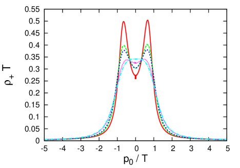
Figure 2: Fermion spectral functions for $g=2$ at $p=0$. The solid (red) curve is for $m_{g}=0$ (tree), the dashed (green) for $m_{g}/T=1/5$, the short-dashed (blue) for $m_{g}/T=1/3$, the dotted (magenta) for $m_{g}/T=g/\sqrt{6}$ and the dot-dashed (cyan) for $m_{g}/T=1$.

To understand the broadening of the peak with increasing value of $m_{g}/T$, we consider the case in which the fermion interacts with HTL corrected gauge boson without continuum parts $\beta_{T}$ and $\beta_{L}$ in Eqs. (12) and (13). We call this gauge boson “HTL pole” gauge boson:

$$\rho_{T}(q_{0},q)\big{|}_{\rm``HTL~{}pole"}=Z_{T}(q)[\delta(q_{0}-\omega_{T}(q))-\delta(q_{0}+\omega_{T}(q))]~{}~{},$$ (20)

$$\rho_{L}(q_{0},q)\big{|}_{\rm``HTL~{}pole"}=Z_{L}(q)[\delta(q_{0}-\omega_{L}(q))-\delta(q_{0}+\omega_{L}(q))]~{}~{}.$$ (21)

On the other hand, the HTL corrected gauge boson with continuum part is labeled as “full HTL” gauge boson:

$$\rho_{T}(q_{0},q)\big{|}_{\rm``full~{}HTL"}=Z_{T}(q)[\delta(q_{0}-\omega_{T}(q))-\delta(q_{0}+\omega_{T}(q))]+\beta_{T}(q_{0},q)~{}~{},$$ (22)

$$\rho_{L}(q_{0},q)\big{|}_{\rm``full~{}HTL"}=Z_{L}(q)[\delta(q_{0}-\omega_{L}(q))-\delta(q_{0}+\omega_{L}(q))]+\beta_{L}(q_{0},q)~{}~{}.$$ (23)

We plot the spectral functions of fermion at $p=0$ coupled with tree gauge boson, the “full HTL” gauge boson and the “HTL pole” gauge boson in Fig. 3.

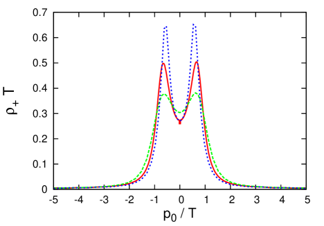
Figure 3: Fermion spectral functions for $g=2$ and $m_{g}/T=1/3$ at $p=0$. Solid (red) curve is the spectrum of fermion coupled with tree gauge boson, dashed (green) curve is coupled with “full HTL” gauge boson expressed in Eqs. (22) and (23), and dotted (blue) curve is coupled with “HTL pole” gauge boson expressed in Eqs. (20) and (21).

The spectral function of fermion interacting with the “HTL pole” gauge boson shown by the dotted (blue) curve in Fig. 3 is sharper than that with tree gauge boson shown by the solid (red) curve. Because the SDE is a self-consistent equation, the internal fermion propagator has a thermal mass. The imaginary part of the fermion self-energy at one-loop, in which both the internal fermion and gauge boson have pole masses (denoted by $m_{f}$ and $m_{g}$), is forbidden in the energy region $|m_{f}-m_{g}|<|p_{0}|<m_{f}+m_{g}$ at $p=0$ owing to the energy-momentum conservation. While the imaginary part in the SDE is not completely forbidden but suppressed in the region, since the internal fermion in the SDE has a width. As was observed in a Yukawa model in Ref. Mitsutani:2007gf, the suppression of the imaginary part leads to a sharp peak in the spectral function. As a result, the peak of the fermion spectrum interacting with the “HTL pole” gauge boson is sharper than that with the tree gauge boson. As $m_{g}$ increases, the above region becomes larger and the peak of fermion spectrum becomes even sharper. When the value of $m_{g}$ is very large, the fermion spectrum will approach that of the free fermion because the gauge boson decouples from the system.

From the above analysis, we find that the continuum parts in Eqs. (22) and (23) play important rolls for the broadening of the fermion spectrum in the case of the “full HTL” gauge boson. Below, we give an interpretation for the broadening of the fermion spectrum with increasing $m_{g}/T$: The dominant parts of $\beta_{T}$ and $\beta_{L}$ are proportional to $m_{g}^{2}$ as we see in Eqs. (14) and (15), i.e. the Landau damping of gauge boson becomes larger as the value of $m_{g}/T$ increases. $m_{g}/T$ is proportional to the coupling at the point indicated by “A” in Fig. 4. [Note that the coupling at “A” is different from $g$.] Therefore the broadening can be interpreted as the increasing probability of scatterings of fermion and gauge boson at “A”. We would like to note that this effects is not included in quenched lattice simulations.

Figure 4: A diagram which generates the imaginary part of the propagator for the fermion interacting with the HTL corrected gauge boson.

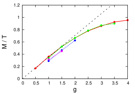
Figure 5: The coupling dependence of the thermal mass $M/T$. The solid (red) curve represents the one for $m_{g}=0$ (tree), the dashed (green) curve for $m_{g}/T=1/3$, the short-dashed (blue) curve for $m_{g}/T=1/2$, the dotted (magenta) curve for $m_{g}/T=1/\sqrt{6}$ and the dashed (black) line represents the thermal mass of fermion in the HTL approximation. In the case of $m_{g}/T=1$, we cannot read the peak as an excitation.

At the last of this section, we consider the coupling dependence (Fig. 5) and the cutoff dependence (Fig. 6) of the peak position of the fermion spectral function which we call the thermal mass. Figure 5 shows that the thermal masses hardly depend on the value of $m_{g}/T$ when the peaks exist as clear ones. On the other hand, the widths strongly depend on $m_{g}/T$ as seen in Fig. 2, and there are no quasi-fermions in the strong coupling region as seen in Fig. 1. That is why the curves for $m_{g}/T>0$ in Fig. 5 terminate at some values of the coupling. This is contrasted to the previous work[8], in which tree gauge boson ($m_{g}/T=0$) was used. There, we saw that the peak position saturates at a value of coupling and the peak position $M$ becomes $M/T\sim 1$ in the very strong coupling region. From Fig. 6, we see that $M/T$ depends little on $\Lambda/T$ in the region $\Lambda/T\gtrsim 4$. We have also checked that the shape of the fermion spectral function around the peak hardly depends on the cutoff.

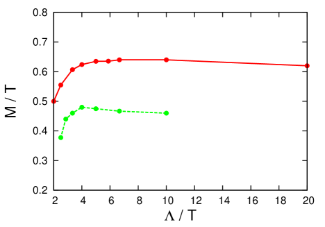
Figure 6: Cutoff dependence of the thermal mass $M/T$. The solid (red) curve is for $m_{g}/T=1/3$ and the dashed (green) for $m_{g}/T=g/\sqrt{6}$. For $\Lambda/T\gtrsim 4$, the ratio $M/T$ is almost independent of the cutoff.

4 A summary and discussions

In this paper, we investigated the fermion spectra in the chiral symmetric phase, focusing on the effect of medium correction for gauge boson, by employing the Schwinger-Dyson equation (SDE) for fermion with the ladder approximation.

We found that in-medium effects for gauge boson propagator make the peak of the fermion spectral function broader compared with the previous result[8] obtained with the tree gauge boson propagator. The broadening occurs owing to multiple fermion-fermion scatterings in addition to fermion-gauge boson scatterings, included through the Landau damping of in-medium corrected gauge boson. Thus, it is important to take into account of not only the thermal mass but also the Landau damping of gauge boson propagator. Our results show no clear peak in the strong coupling region, which implies the disappearance of quasi-fermions in the strongly coupled plasma.

We would like to make a comment on the Van Hove singularities. They exist in the case of the self-energy consisting of two very sharp particles whose dispersion relations are different from each other as in the fermion and gauge boson in the HTL approximation. However, if the particles have widths, these singularities are weakened. In the SDE, because the (internal) fermion has a broad width by non-perturbative effects through the self-consistency condition, we cannot see the effects of Van Hove singularities in the present analysis.

In this paper, we solved the SDE in the Minkowski space as an iterative equation for the fermion spectral function. In the previous work[8], on the other hand, the solution is obtained by performing the analytic continuation from the imaginary time axis to the real time axis through an integral equation. There is little difference in the fermion spectra obtained by two methods as seen in appendix B. We also show that there is little gauge dependence of the peak position in appendix B.

We discuss the application of the results of the present work to QCD. In the very high temperature region of QCD, the HTL approximation is valid for studying the quark spectrum. In the HTL approximation, the fixed coupling, which is the running coupling at an energy scale of order $T$, say $g(T)$, is used, because the quarks and gluons with energy $T$ give the dominant contribution. In studying the quark spectrum in the lower $T$ region, the diagrams other than the HTL start to give non-negligible corrections, since the (fixed) coupling $g(T)$ is larger. For this reason, we can state that, in our approach, we include a part of non-perturbative corrections from a certain diagrams by solving the Schwinger-Dyson equation. However, the following points of QCD are not included: (1) the asymptotic freedom through the running effects of the gauge coupling, (2) vertex corrections and (3) higher oder corrections for the gauge boson.

First, we discuss the effect of asymptotic freedom. In our analysis, the fixed coupling is used, which can be understood as the running coupling at an energy scale of oder $T$, i.e. $g(T)$. In the energy scale $E$ lower than $T$, the gauge coupling does not run, and we have $g(E)\sim g(T)$. This is because quarks and gluons decouple in this energy region owing to the thermal mass. In $E\gtrsim T$, gauge coupling is running, and we have $g(E)<g(T)$. The difference between $g(E)$ and $g(T)$ might cause different results when we use the running coupling in the SDE analysis. However, in the present analysis, we have seen that peak position only depend on $T$ which is an infrared scale, but does not depend on the cutoff $\Lambda$ which is an ultraviolet scale: The peak position is determined by the dynamics of the infrared scale only. Therefore, we think that the peak positions at least will hardly change from those in the present analysis.

Second, we discuss vertex corrections. When we take account of some vertex corrections, the peak of fermion spectrum will become even broader than that in the present analysis owing to multiple scatterings. Then the following qualitative structure of the quark spectrum will hardly change: The peak position of the quark is proportional to the coupling for small $g(T)$ and the quasi-particle picture will be even worse.

Third, we discuss higher order corrections for the gauge boson propagator. There is a coupled SDE for fermion and gauge boson, in which we can include certain higher order corrections for the gauge boson propagator. The peak of fermion spectrum will become even broader than that in the present analysis owing to multiple scatterings. The peak position does not depend on a detailed structure of gauge boson propagator in the present analysis, which indicates that the peak position does not change from the present value in the small coupling region, and that the quasi-particle picture will not be good in the strong coupling region.

To summarize, the following qualitative structure of the quark spectrum will hold in hot QCD: In the high $T$ region where $g(T)$ is small, the thermal masses of the quasi-quark and the plasmino are proportional to the coupling. In the low $T$ region where $g(T)$ is large, the width will become broad due to multiple scatterings. Especially, in the strongly coupled QGP near $T_{c}$, the quasi-particle picture may be no longer valid.

It is suggested that bound states for light quarks exist near $T_{c}$ in Ref. Shuryak:2004cy and Brown:2003km. It is also suggested that new mesonic states consisting of a quark and a plasmino exist in Ref. Weldon:1998ic. It is very interesting to study these bound states for light quarks through the Bethe-Salpeter equation using the fermion spectra obtained in the present analysis.

Appendix A The SDE in the imaginary time formalism and the chiral phase transition

In this appendix, we determine the critical temperature $T_{c}$ of the chiral phase transition from the ladder SDE. We solve the SDE in the imaginary time formalism because the numerical cost is much smaller than solving the SDE on the real time axis.

The ladder SDE in the imaginary time formalism is given by Eq. (1). The full fermion propagator in the imaginary time formalism is restricted by the rotational invariance and the parity invariance as follows:

$${\mathcal{S}}(i\omega_{n},\vec{p})=\frac{1}{B(i\omega_{n},p)+A(i\omega_{n},p)\vec{p}\cdot\vec{\gamma}-C(i\omega_{n},p)i\omega_{n}\gamma_{0}}.$$ (24)

The HTL corrected gauge boson propagator in the Coulomb gauge is expressed as

$${\mathcal{D}}^{\mu\nu}(i\omega_{n}-i\omega_{m},\vec{p}-\vec{k}) =\Delta_{T}(i\omega_{n}-i\omega_{m},\vec{p}-\vec{k})P^{\mu\nu}_{T}+\Delta_{L}(i\omega_{n}-i\omega_{m},\vec{p}-\vec{k})\delta^{\mu 0}\delta^{\nu 0},$$ (25)

where $\Delta_{T}$ and $\Delta_{L}$ are transverse and longitudinal HTL corrected gauge boson propagators. They are expressed as

$$\Delta_{T}(i\omega,q) =\frac{1}{\omega^{2}+q^{2}+m_{g}^{2}\Biggl{(}-\frac{\omega^{2}}{q^{2}}+\left(1+\frac{\omega^{2}}{q^{2}}\right)\frac{|\omega|}{2q}\left(\pi-2\tan^{-1}\frac{|\omega|}{q}\right)\Biggr{)}},$$ (26)

$$\Delta_{L}(i\omega,q) =\frac{-1}{q^{2}+2m_{g}^{2}\Biggl{(}1-\frac{|\omega|}{2q}\left(\pi-2\tan^{-1}\frac{|\omega|}{q}\right)\Biggr{)}}.$$ (27)

Note that Eq. (26) and Eq. (27) have no poles for real $\omega$. Using these fermion propagator and gauge boson propagators, the ladder SDE (1) is decomposed into three coupled equations for $B$, $A$ and $C$ as

$$B =g^{2}T\sum_{m=-\infty}^{\infty}\int\frac{d^{3}k}{(2\pi)^{3}}\frac{B}{B^{2}+C^{2}\omega_{m}^{2}+A^{2}k^{2}}\left[2\Delta_{T}-\Delta_{L}\right],$$ (28)

$$A =1+\frac{g^{2}T}{p^{2}}\sum_{m=-\infty}^{\infty}\int\frac{d^{3}k}{(2\pi)^{3}}\frac{A}{B^{2}+C^{2}\omega_{m}^{2}+A^{2}k^{2}}\left[2\Delta_{T}\left(\frac{(\vec{p}\cdot\vec{q})(\vec{k}\cdot\vec{q})}{q^{2}}\right)-\Delta_{L}\vec{p}\cdot\vec{k}\right],$$ (29)

$$C =1+\frac{g^{2}T}{p_{0}}\sum_{m=-\infty}^{\infty}\int\frac{d^{3}k}{(2\pi)^{3}}\frac{Ck_{0}}{B^{2}+C^{2}\omega_{m}^{2}+A^{2}k^{2}}\left[2\Delta_{T}+\Delta_{L}\right].$$ (30)

Because the integrals in Eqs. (28)–(30) are divergent, we introduce the three-dimensional ultraviolet cutoff $\Lambda$. We also truncate the infinite sum of the Matsubara frequency at a finite number $N$. However, $N$ can be taken to be sufficiently large so that the following results do not depend on it. The angle integral in Eqs. (28)–(30) are numerically performed.

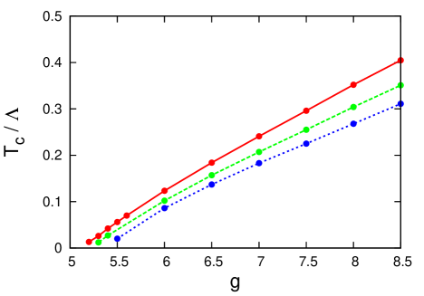
Figure 7: Coupling dependence of the critical temperature $T_{c}/\Lambda$. The chiral symmetric (broken) phase is above (below) the line. The solid (red) line shows $T_{c}/\Lambda$ for $m/\Lambda=0$, the dashed (green) line for $m/\Lambda=0.1$ and the dotted (blue) line for $m_{g}/\Lambda=0.2$.

In Fig. 7, we plot the coupling dependence of $T_{c}/\Lambda$ for $m_{g}/\Lambda=0,~{}0.1$ and $0.2$. We see that $T_{c}/\Lambda$ decreases as $m_{g}/\Lambda$ increases owing to the screening effects. This is consistent with the results in Ref. Takagi which show that $T_{c}$ becomes small by the effects of the Debye screening.

Appendix B Dependences on the gauge fixing condition and method for solving the SDE

There are two methods to obtain the solutions of the SDE on the real time axis. One is to perform the analytic continuation for the solutions of the SDE in the imaginary time formalism through an integral equation[21], which was used in the previous work[8]. Another method is to solve a self-consistent equation as an integral equation for fermion spectral function[9]. In this appendix, we show that the dependence of the peak position of the fermion spectral functions on two methods together with the gauge dependence of the peak position. In Fig. 8, we plot the peak positions of fermion spectral functions obtained by the method 1 in the Feynman gauge, by the method 2 in the Feynman gauge and by the method 2 in the Coulomb gauge. We find that the peak positions little depend on neither the method nor the gauge fixing. This is consistent with the result of Ref. Baym:1992eu in which the exact calculation of the fermion self-energy at one-loop level is performed and it is shown that the peak positions little depend on the gauge choice.

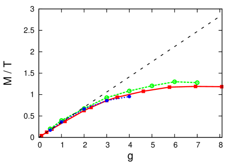
Figure 8: Coupling dependence of the thermal mass. The solid (red) curve represent the thermal mass obtained by the method 1 in the Feynman gauge. The dashed (green) curve and dotted (blue) curve represent the thermal mass obtained by the method 2, in the Feynman and Coulomb gauge, respectively. The dashed (black) line represents the thermal mass in the HTL approximation.

References

- [1] V. V. Klimov, Sov. J. Nucl. Phys. 33 (1981), 934; Yadern. Fiz. 33 (1981), 1734. H. A. Weldon, Phys. Rev. D 26 (1982), 1394. H. A. Weldon, Phys. Rev. D 26 (1982), 2789. H. A. Weldon, Phys. Rev. D 40 (1989), 2410.
- [2] M. Le Bellac, Thermal Field Theory (Cambridge University press, Cambridge, England, 1996).
- [3] I. Arsene et al., Nucl. Phys. A 757 (2005), 1. B. B. Back et al., Nucl. Phys. A 757 (2005), 28. J. Adams et al., Nucl. Phys. A 757 (2005), 102. K. Adcox et al., Nucl. Phys. A 757 (2005), 184.
- [4] T. Umeda, K. Nomura and H. Matsufuru, Eur. Phys. J. C 39S1 (2005), 9 [arXiv:hep-lat/0211003]. M. Asakawa and T. Hatsuda, Phys. Rev. Lett. 92 (2004), 012001 [arXiv:hep-lat/0308034]. S. Datta, F. Karsch, P. Petreczky and I. Wetzorke, Phys. Rev. D 69 (2004), 094507 [arXiv:hep-lat/0312037]. H. Iida, T. Doi, N. Ishii, H. Suganuma and K. Tsumura, Phys. Rev. D 74 (2006), 074502. A. Jakovac, P. Petreczky, K. Petrov and A. Velytsky, Phys. Rev. D 75 (2007), 014506. G. Aarts, C. Allton, M. B. Oktay, M. Peardon and J. I. Skullerud, Phys. Rev. D 76 (2007), 094513
- [5] A. Schaefer and M. H. Thoma, Phys. Lett. B 451 (1999), 195. A. Peshier and M. H. Thoma, Phys. Rev. Lett. 84 (2000), 841.
- [6] M. Mannarelli and R. Rapp, Phys. Rev. C 72 (2005), 064905.
- [7] M. Kitazawa, T. Kunihiro and Y. Nemoto, Phys. Lett. B 633 (2006), 269.
- [8] M. Harada, Y. Nemoto and S. Yoshimoto, Int. J. Mod. Phys. E 16 (2007), 2282 [arXiv:hep-ph/0702253]. M. Harada, Y. Nemoto and S. Yoshimoto, Prog. Theor. Phys 119 (2008), 117. arXiv:0708.3351 [hep-ph].
- [9] M. Harada and Y. Nemoto, Phys. Rev. D 78 (2008) 014004.
- [10] F. Karsch and M. Kitazawa, Phys. Lett. B 658 (2007), 45.
- [11] See, e.g., T. Kugo, in Proc. of 1991 Nagoya Spring School on Dynamical Symmetry Breaking, Nakatsugawa, Japan, 1991, ed. K. Yamawaki (World Scientific, Singapore, 1992). V. A. Miransky, Dynamical symmetry breaking in quantum field theories (Singapore, Singapore: World Scientific, 1993).
- [12] M. Harada and A. Shibata, Phys. Rev. D 59 (1999), 014010. C. D. Roberts and S. M. Schmidt, Prog. Part. Nucl. Phys. 45 (2000), S1.
- [13] M. Harada and S. Takagi, Prog. Theor. Phys. 107 (2002), 561.
- [14] S. Takagi, Prog. Theor. Phys. 109 (2003), 233.
- [15] T. Ikeda, Prog. Theor. Phys. 107 (2002), 403. Y. Fueki, H. Nakkagawa, H. Yokota and K. Yoshida, Prog. Theor. Phys. 110 (2003), 777.
- [16] H. Nakkagawa, H. Yokota and K. Yoshida, in the Proceedings of the 2006 International Workshop ”The Origin of Mass and Strong Coupling Gauge Theories,” Nagoya, Japan, 2006, ed. M. Harada, M. Tanabashi and K. Yamawaki (World Scientific, Singapore, 2008), p. 220 [hep-ph/0703134.] H. Nakkagawa, H. Yokota and K. Yoshida, in the Proceedings of the Nagoya Mini-workshop ”Strongly Coupled Quark-Gluon Plasma: SPS, RHIC and LHC,” Nagoya, Japan, 2007, ed. C. Nonaka and M. Harada, p. 173 [arXiv:0707.0929]. H. Nakkagawa, H. Yokota and K. Yoshida, arXiv:0709.0323 [hep-ph].
- [17] M. Kitazawa, T. Kunihiro and Y. Nemoto, Prog. Theor. Phys. 117 (2007), 103. M. Kitazawa, T. Kunihiro, K. Mitsutani and Y. Nemoto, Phys. Rev. D 77 (2008), 045034.
- [18] E. V. Shuryak and I. Zahed, Phys. Rev. C 70 (2004), 021901; Phys. Rev. D 70 (2004), 054507.
- [19] G. E. Brown, C. H. Lee, M. Rho and E. Shuryak, Nucl. Phys. A 740 (2004), 171; J. Phys. G 30 (2004), S1275. H. J. Park, C. H. Lee and G. E. Brown, Nucl. Phys. A 763 (2005), 197. G. E. Brown, B. A. Gelman and M. Rho, Phys. Rev. Lett. 96 (2006), 132301. G. E. Brown, C. H. Lee and M. Rho, arXiv:nucl-th/0507011.
- [20] H. A. Weldon, arXiv:hep-ph/9810238.
- [21] F. Marsiglio, M. Schossmann and J. P. Carbotte, Phys. Rev. B 37 (1988), 4965.
- [22] G. Baym, J. P. Blaizot and B. Svetitsky, Phys. Rev. D 46 (1992), 4043.