Vertex corrections of impurity scattering at a ferromagnetic quantum critical point

Abstract

We study the renormalization of a non-magnetic impurity’s scattering potential due to the presence of a massless collective spin mode at a ferromagnetic quantum critical point. To this end, we compute the lowest order vertex corrections in two- and three-dimensional systems, for arbitrary scattering angle and frequency of the scattered fermions, as well as band curvature. We show that only for backward scattering in $D=2$ does the lowest order vertex correction diverge logarithmically in the zero frequency limit. In all other cases, the vertex corrections approach a finite (albeit possibly large) value for $\omega\rightarrow 0$. We demonstrate that vertex corrections are strongly suppressed with increasing curvature of the fermionic bands. Moreover, we show how the frequency dependence of vertex corrections varies with the scattering angle. We also discuss the form of higher order ladder vertex corrections and show that they can be classified according to the zero-frequency limit of the lowest order vertex correction. We show that even in those cases where the latter is finite, summing up an infinite series of ladder vertex diagrams can lead to a strong enhancement (or divergence) of the impurity’s scattering potential. Finally, we suggest that the combined frequency and angular dependence of vertex corrections might be experimentally observable via a combination of frequency dependent and local measurements, such as scanning tunneling spectroscopy on ordered impurity structures, or measurements of the frequency dependent optical conductivity.

I Introduction

Understanding the complex physical properties of materials near a quantum critical point (QCP) is one of the most important open problems in condensed matter physics (for a recent review, see Loe07 and references therein). An important piece of this puzzle is the question of how soft collective fluctuations associated with the proximity of the QCP affect the scattering potential of non-magnetic impurities Miyake:2001 ; Kim:2003 . The answer to this question is of great significance for a series of experimental probes, ranging from measurements of the residual resistivity Paul et al. (2005); Belitz et al. (2000) and optical conductivity to that of the local density of states near impurities. Indeed, it was recently argued by Kim and Millis Kim:2003 that the transport anomalies observed at the metamagnetic transition of ${\rm Sr_{3}Ru_{2}O_{7}}$ Perry and et al. (2001); Grigera and et al. (2001) arise from a diverging renormalization of the impurities’ scattering potential.

In this article we study the renormalization of a non-magnetic impurity’s scattering potential due to the presence of a massless collective spin mode at a ferromagnetic quantum critical point (FMQCP). To this end, we compute both analytically and numerically, the lowest order vertex corrections in two- and three-dimensional systems, for arbitrary scattering angle and frequency of the scattered electrons, as well as curvature of the fermionic band. We limit ourselves to the case of a vanishing impurity density such that the nature of the QCP is not altered by the presence of the impurities. Moreover, since the renormalization of the impurity potential by a collective mode effectively enlarges the size of the impurity in real space, the limit of vanishing impurity density also guarantees that quantum interference effects between impurities can be omitted. The interaction of a soft collective spin mode with the fermionic degrees of freedom in the vicinity of a FMQCP was studied previously Rou01 ; Wang01 ; Chu03 ; Dze04 ; Chu05 (for related work in the context of gauge theories see Lee89 ; Blo93 ; Khv94 ; Nay94 ; Alt95 ). At the FMQCP, the same collective spin mode that renormalizes the impurity’s scattering potential yields self-energy corrections to the electronic Greens functions that render the latter non-Fermi-liquid (NFL) like Lee89 ; Alt95 . In order to investigate how the NFL nature of the fermions affect the vertex corrections, we contrast them with those obtained using a Fermi-liquid (FL) form of the fermionic propagators. By doing so, we make contact with two earlier studies of vertex corrections near a FMQCP. Specifically, Miyake et al. Miyake:2001 , using a FL form of the fermionic propagators, studied vertex corrections for forward scattering near a FMQCP in $D=3$, while Kim and Millis Kim:2003 investigated the vertex renormalization for backward scattering in $D=2$ at zero frequency.

We obtain a number of interesting results. First, we find that only for backward scattering in $D=2$ does the lowest order vertex correction diverge in the limit of vanishing frequency. This divergence is logarithmic both for the NFL and the FL case. In all other cases, the vertex corrections approach a finite (albeit possibly large) value for $\omega\rightarrow 0$, with the overall scale for vertex corrections being smaller in the NFL than in the FL case. This result is in disagreement with the earlier finding of Miyake et al. Miyake:2001 who reported a logarithmic divergence in frequency for forward scattering in $D=3$. Second, vertex corrections are in general strongly suppressed with increasing curvature of the fermionic bands. For backward scattering, this suppression obeys a qualitatively different functional form in the NFL and FL cases. Third, we identify the combined dependence of the vertex corrections on scattering angle, frequency, and band curvature. Fourth, we discuss the form of higher order ladder vertex corrections and show that they can be classified according to the zero-frequency limit of the lowest order vertex correction. We show that even in those cases where the latter is finite, summing up an infinite series of ladder vertex diagrams can lead to a strong enhancement (or divergence) of the impurity’s scattering potential. Finally, we suggest that the combined frequency and angular dependence of vertex corrections might be experimentally observable via a combination of frequency dependent and local measurements, such as scanning tunneling spectroscopy (STS) on ordered impurity structures, or measurements of the frequency dependent optical conductivity.

While we consider below a FMQCP with a ${\bf q}=0$ ordering wavevector, the question of whether such a QCP is actually realized in nature has attracted significant interest over the last few years. In the standard theoretical approaches Hertz (1976); Millis (1993) such a QCP is described by integrating out the electronic degrees of freedom and deriving a low energy Landau-Ginzburg effective action in terms of the order parameter field. A number of recent studies Belitz et al. (1997); Coleman:2001 ; Abanov et al. (2003); Chubukov and Maslov (2003) (for reviews see Abanov et al. (2003); Belitz et al. (2002, 2005); Rech et al. (2006)) have shed some doubt on the validity of this approach since they argued that for a system with an SU(2) (Heisenberg) spin symmetry, the momentum dependence of the static spin susceptibility acquires negative non-analytic corrections. These corrections could either lead to a first-order transition in the ferromagnetic state, or could give rise to an incommensurate order with non-zero ordering wavevector. In contrast, in systems with an Ising spin symmetry, these corrections are absent, and a $({\bf q}=0)$-FMQCP can in general occur. A candidate system for the latter case is ${\rm Sr_{3}Ru_{2}O_{7}}$, which exhibits a metamagnetic transition. While this transition is in general first order in nature, it can be tuned to a critical end point which is located close to $T=0$, thus representing a (quasi) quantum critical point. At the same time, the externally applied field renders the spin symmetry Ising-like. In order to keep the discussion of our results as general as possible, we explicitly show below how the spin symmetry of a system, Heisenberg-, XY- or Ising-like, affects the form of the vertex corrections.

The rest of the paper is organized as follow. In Sec. II we give a brief derivation of the bosonic and fermionic propagators at the FMQCP in $D=2$ and $3$. In Sec. III we present the general expression for the lowest order vertex correction, ${\Delta\Gamma}$, that we employ for our numerical and analytical calculations. In Secs. IV and V we present the results for vertex corrections in $D=2$ and $D=3$, respectively, as a function of scattering angle, frequency and band curvature. In Sec. VI we discuss the form of the higher order vertex corrections and their effects on the renormalized scattering potential. Finally, in Sec. VII we summarize our findings and discuss their implications for transport and STS experiments.

II Spin susceptibility and fermionic self energy

Our starting point is the spin-fermion model (for details, see, e.g., Ref. Abanov et al. (2003); Rech et al. (2006)) whose Hamiltonian is given by

$$H= \sum_{{\rm\bf k}\sigma}\epsilon_{\rm\bf k}c^{\dagger}_{{\rm\bf k}\sigma}c_{{\rm\bf k}\sigma}+\sum_{q}\chi_{0}({\rm\bf q})^{-1}{\rm\bf S}_{\rm\bf q}{\rm\bf S}_{-{\rm\bf q}}$$

$$+g\sum_{{\rm\bf k},{\rm\bf q},\sigma,\sigma^{\prime}}c^{\dagger}_{{\rm\bf k}\sigma}{\bf\tau}_{\sigma\sigma^{\prime}}c_{{\rm\bf k}+{\rm\bf q},\sigma^{\prime}}\cdot{\rm\bf S}_{\rm\bf q}\quad,$$ (1)

where $c^{\dagger}_{{\bf k},\sigma}$, ($c_{{\bf k},\sigma}$) is the fermionic creation (annihilation) operator for an electron with momentum ${\bf k}$ and spin $\sigma$, ${\rm\bf S}_{q}$ are vector bosonic operators, $g$ is the effective fermion-boson coupling, ${\bf\tau}_{\sigma\sigma^{\prime}}$ are the Pauli matrices, and

$$\chi_{0}({\rm\bf q})=\frac{\chi_{0}}{\xi^{-2}+q^{2}}$$ (2)

is the static propagator describing ferromagnetic fluctuations, with $\xi$ being the magnetic correlation length. While, in general, $\chi_{0}({\rm\bf q})$ could be obtained by integrating out the high-energy fermions (for a more detailed discussion, see Ref.Rech et al. (2006)), it is commonly used as a phenomenological input for the model. The above model describes the low-energy excitations of the system (such that $|{\rm\bf q}|<W/v_{F}$ where $W$ is of the order of the fermionic bandwidth and $v_{F}$ is the Fermi velocity), in which the dynamic part of bosonic propagator is generated by the interaction with the low-energy fermions. The full bosonic propagator is thus obtained via the Dyson equation

$$\chi^{-1}({\rm\bf q},i\Omega_{m})=\chi^{-1}_{0}({\rm\bf q})-\Pi({\rm\bf q},i\Omega_{m})\quad,$$ (3)

where $\Pi({\rm\bf q},i\Omega_{m})$ is the bosonic self-energy (the polarization operator) which to lowest order in $g$ is given by

$$\Pi({\rm\bf q},i\Omega_{m})= -g^{2}T\sum_{n}\int\frac{d^{D}k}{(2\pi)^{d}}\ G_{0}({\rm\bf k},i\omega_{n})$$

$$\times G_{0}({\rm\bf k}+{\rm\bf q},i\omega_{n}+i\Omega_{m})\quad,$$ (4)

where $G_{0}({\rm\bf k},i\omega_{n})=(i\omega_{n}-\epsilon_{\rm\bf k})^{-1}$ is the bare Green’s function for the fermions, $\omega_{n}$ ($\Omega_{m}$) is the fermionic (bosonic) Matsubara frequency, and $D$ is the dimensionality of the system. In the remainder of the paper, we set $\xi\to\infty$ and study the form of vertex corrections for impurity scattering at the FMQCP.

In the limit $T\to 0$, the polarization bubble can easily be evaluated (see, for example, Abanov et al. (2003); Rech et al. (2006)). After expanding the fermionic dispersion as

$$\epsilon_{\rm\bf k}\approx v_{F}({\rm\bf k})k_{\parallel}+r({\rm\bf k})(k_{\parallel}^{2}+k_{\perp}^{2})\quad,$$ (5)

where $v_{F}({\rm\bf k})$ and $r({\rm\bf k})$ are the local Fermi velocity and band curvature, respectively, and $k_{\parallel}$ ($k_{\perp}$) is the component of ${\rm\bf k}$ parallel (perpendicular) to the normal of the Fermi surface, and keeping only terms in $G_{0}$ up to linear order in ${\rm\bf q}$, one obtains for an isotropic system (i.e., for constant $v_{F}$ and $r$) in $D=2$

$$\Pi({\rm\bf q},i\Omega_{m})=-2g^{2}N_{0}\frac{|\Omega_{m}|}{\sqrt{\Omega_{m}^{2}+(v_{F}q)^{2}}}\quad,$$ (6)

while for $D=3$ one has

$$\Pi({\rm\bf q},i\Omega_{m})=i\frac{g^{2}N_{0}|\Omega_{m}|}{v_{F}q}\ln\left(\frac{1-i\frac{\Omega_{m}}{v_{F}q}}{-1-i\frac{\Omega_{m}}{v_{F}q}}\right)\quad,$$ (7)

where $q=|{\bf q}|$, and $N_{0}$ is the density of states. We assume $rq/v_{F}\ll 1$ such that the local curvature $r$ of the fermionic dispersion leads to only subleading corrections to $\Pi$, which can be neglected Rech et al. (2006). In the limit $\Omega_{m}\ll v_{F}q$ we can simplify the above expressions, and obtain for $D=2$ from Eq.(6) Chu05

$$\Pi({\rm\bf q},i\Omega_{m})=-2g^{2}N_{0}\frac{|\Omega_{m}|}{v_{F}q}$$ (8)

and for $D=3$ from Eq.(7)

$$\Pi({\rm\bf q},i\Omega_{m})=-\pi g^{2}N_{0}\frac{|\Omega_{m}|}{v_{F}q}\quad.$$ (9)

In order to simplify the notation, we introduce the Landau damping parameter $\lambda$ such that for $D=2$ one has $\lambda\equiv 2\chi_{0}g^{2}N_{0}$ while for $D=3$ one obtains $\lambda\equiv\pi\chi_{0}g^{2}N_{0}$, the difference being only a numerical factor. At the QCP, the full spin susceptibility is then given by

$$\chi({\rm\bf q},i\Omega_{m})=\frac{\chi_{0}}{q^{2}+\lambda\frac{|\Omega_{m}|}{v_{F}q}}\ .$$ (10)

Using this form of $\chi$, we can now compute the lowest order fermionic self energy correction, $\Sigma$, shown in Fig.1(a),

Figure 1: (a) Diagram for the lowest order self energy correction. (b) Example of rainbow diagram. (c) Example of neglected higher order corrections.

which for $T=0$ is given by

$$\Sigma({\rm\bf k},i\omega_{n})=I_{s}\ g^{2}\int\frac{d^{D}p\ d\nu_{m}}{(2\pi)^{D+1}}\chi({\rm\bf k}+{\rm\bf p},i\omega_{n}+i\nu_{m})G({\rm\bf p},i\nu_{m})\ ,$$ (11)

with $I_{s}=1,2$ or 3 for a system with Ising, XY or Heisenberg spin symmetry, respectively. In the limit $\lambda/k_{F}^{2}\ll 1$, typical bosonic momenta are much bigger than typical fermionic momenta Rech et al. (2006), and one can decouple the momentum integration parallel and perpendicular to the normal of the Fermi surface by setting

$$\chi(p_{\perp},p_{\parallel},i\Omega_{m})\approx\chi(p_{\perp},0,i\Omega_{m})\ .$$ (12)

This yields

$$\Sigma({\rm\bf k},i\omega_{n})= I_{s}g^{2}\int\frac{d^{D-1}p_{\perp}d\nu_{m}}{(2\pi)^{D}}\chi(p_{\perp},i\nu_{m}+i\omega_{n})$$

$$\times\int_{-\infty}^{\infty}\frac{dp_{\parallel}}{2\pi}G(p_{\parallel},i\nu_{m}).$$ (13)

Using $G(p_{\parallel},i\omega_{n})=1/(i\omega_{n}-v_{F}p_{\parallel})$, one obtains from Eq.(13) in $D=2$ (see Ref.Lee89 ; Alt95 )

$$\Sigma({\rm\bf k},i\omega_{n})=-i\omega_{0}^{1/3}|\omega_{n}|^{2/3}{\rm sgn}(\omega_{n})$$ (14)

where

$$\omega_{0}\equiv\frac{I^{3}_{s}}{3\sqrt{3}(4\pi)^{3}}\frac{\lambda^{2}}{v_{F}^{2}N_{0}^{3}}=\frac{I^{3}_{s}}{12\sqrt{3}}\ \alpha^{2}E_{F}\ ,$$ (15)

$\alpha=\lambda/k_{F}^{2}$, and $E_{F}=v_{F}k_{F}/2$ is the Fermi energy. $\omega_{0}$ is interpreted as the upper frequency scale for quantum critical behavior since for $\omega<\omega_{0}$ the fermions possess a non-Fermi liquid character, while for $\omega>\omega_{0}$ the Fermi liquid behavior is recovered. For $D=3$, one has

$$\Sigma({\rm\bf q},i\omega_{n})=-i\gamma\,\omega_{n}\,\ln\left(1+\frac{\Omega_{c}}{|\omega_{n}|}\right)$$ (16)

with

$$\gamma\equiv\frac{I_{s}g^{2}\chi_{0}}{12\pi^{2}v_{F}}=I_{s}\frac{\lambda}{6\pi k_{F}^{2}};\quad\Omega_{c}\equiv\frac{v_{F}\Lambda^{3}}{\lambda}\ .$$ (17)

Here, $\Lambda$ is a momentum cutoff of order $1/a_{0}$, where $a_{0}$ is the lattice constant. In $D=3$ the upper frequency scale for quantum critical behavior is given by

$$\omega_{0}\equiv\Omega_{c}e^{-1/\gamma}.$$ (18)

As discussed above, this derivation of the self-energies only holds in the limit $\lambda/k_{F}^{2}\ll 1$, implying $\alpha\ll 1$ in $D=2$ and $\gamma\ll 1$ in $D=3$.

Finally, we briefly comment on the effect of higher order self-energy diagrams. It turns out that rainbow diagrams, such as the one shown in Fig.1(b), vanish identically as long as the lowest order self-energy in Fig.1(a) (which is an internal part of all rainbow diagrams) is independent of $k_{\parallel}$; in this case the poles of the internal Greens functions all lie in the same half of the complex plane. In contrast, crossing diagrams such as the one shown in Fig.1(c), provide a renormalization of the boson-fermion vertex, $g$, whose discussion is beyond the scope of this article.

III Vertex corrections for Scattering of Non-Magnetic Impurities

We next consider the scattering of a single non-magnetic impurity, located at ${\bf R}$. The bare scattering process is described by the Hamiltonian ${\cal H}_{imp}=\sum_{\sigma}U_{0}c^{\dagger}_{\sigma}({\bf R})c_{\sigma}({\bf R})$ with bare scattering vertex $U_{0}$, and represented by the diagram shown in Fig. 2(a). The diagrams shown in Fig. 2(b)-(d) represent processes involving the soft ferromagnetic mode that renormalize the impurity’s scattering potential. Note that these processes lead to a renormalized scattering vertex which depends on two additional spatial coordinates, ${\bf r}$ and ${\bf r}^{\prime}$ as shown in Fig. 2(b), effectively leading to an increase in the spatial size of the impurity.

We begin by studying the form of the lowest order vertex correction, $-{\Delta\Gamma}$, shown in Fig. 2(b). Up to second order in $g$, the full vertex, $U$, is then given by

$$U=U_{0}\left(1+\frac{{\Delta\Gamma}}{U_{0}}+...\right)\quad.$$ (19)

Fourier transformation of ${\Delta\Gamma}$ into momentum space yields at $T=0$ (where the fermionic Matsubara frequency $\nu_{m}$ is now a continuous variable)

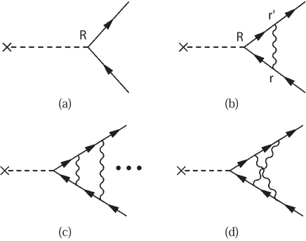
Figure 2: (a) Bare vertex. (b) Lowest order correction to the impurity scattering vertex due the exchange of soft magnetic fluctuations. (c) and (d) higher order diagrams: ladder (c), and crossed (d).

$$\frac{{\Delta\Gamma}({\bf p},{\rm\bf k},i\omega_{n})}{U_{0}}= -I_{s}g^{2}\int\frac{d^{D}q}{(2\pi)^{D}}\int\frac{d\nu_{m}}{2\pi}\chi({\rm\bf q},i\nu_{m}-i\omega_{n})$$

$$G({\rm\bf p}-{\rm\bf q}-{\rm\bf k}/2,i\nu_{m})G({\rm\bf p}-{\rm\bf q}+{\rm\bf k}/2,i\nu_{m})$$ (20)

with momentum transfer ${\rm\bf k}$ at the impurity. In order to evaluate ${\Delta\Gamma}$, we write $G$ in the general form

$$G({\rm\bf k},i\nu_{m})=\frac{1}{Z(i\nu_{m})-\epsilon_{k}}\quad,$$ (21)

where $Z(i\nu_{m})=i\nu_{m}$ in the Fermi-liquid regime, and $Z(i\nu_{m})=i\nu_{m}+\Sigma(i\nu_{m})$ in the non-Fermi liquid regime. Here, $\Sigma$ for $D=2$ is given by Eq.(14) and for $D=3$ by Eq.(16). In what follows, we study ${\Delta\Gamma}$ for fermions near the Fermi surface, and hence set $\left|{\rm\bf p}-{\rm\bf k}/2\right|\sim p_{F}$ and $\left|{\rm\bf p}+{\rm\bf k}/2\right|\sim p_{F}$. We can then expand the dispersion entering the Greens functions in Eq.(20) as

$$\epsilon_{{\rm\bf p}-{\rm\bf q}-{\rm\bf k}/2} \sim -v_{F}q\cos\theta+rq^{2}$$

$$\epsilon_{{\rm\bf p}-{\rm\bf q}+{\rm\bf k}/2} \sim -v_{F}q\cos(\theta+\varphi)+rq^{2}\quad,$$ (22)

where $\varphi$ is the scattering angle and $\theta$ is the angle between ${\rm\bf p}-{\rm\bf k}/2$ and ${\rm\bf q}$. With these approximations and the expression given in Eq.(10) for the bosonic propagator, we obtain in $D=2$

$$\frac{{\Delta\Gamma}}{U_{0}}= -\frac{I_{s}g^{2}\chi_{0}}{(2\pi)^{3}}\int_{0}^{q_{max}}dq\int_{-\omega_{max}}^{\omega_{max}}d\nu_{m}\frac{q^{2}}{q^{3}+\frac{\lambda}{v_{F}}|\nu_{m}-\omega_{n}|}$$

$$\times\int_{0}^{2\pi}d\theta\frac{1}{Z(\nu_{m})+v_{F}q\cos\theta-rq^{2}}\cdot$$

$$\times\frac{1}{Z(\nu_{m})+v_{F}q\cos(\theta+\varphi)-rq^{2}}\quad,$$ (23)

while for $D=3$, one has

$$\frac{{\Delta\Gamma}}{U_{0}}= -\frac{I_{s}g^{2}\chi_{0}}{(2\pi)^{3}}\int_{0}^{q_{max}}dq\int_{-\omega_{max}}^{\omega_{max}}d\nu_{m}\frac{q^{3}}{q^{3}+\frac{\lambda}{v_{F}}|\nu_{m}-\omega_{n}|}$$

$$\times\int_{-1}^{1}d(\cos\theta)\frac{1}{Z(\nu_{m})+v_{F}q\cos\theta-rq^{2}}\cdot$$

$$\times\frac{1}{Z(\nu_{m})+v_{F}q\cos(\theta+\varphi)-rq^{2}}\quad.$$ (24)

Here, $q_{max}$ and $\omega_{max}$ are cut-offs in momentum and frequency space, respectively. All numerical results presented below for $\Delta\Gamma$ in $D=2$ are obtained from Eq.(23) with $Z(\nu_{m})=i\nu_{m}$ for the FL case, and $Z(\nu_{m})=i\nu_{m}+i\omega_{0}^{1/3}|\nu_{m}|^{2/3}{\rm sgn}(\nu_{m})$ for the NFL case com2 . Moreover, after rescaling all frequencies with $\omega_{0}$ and all momenta with $q_{0}=\omega_{0}/v_{F}$, one finds that the above integral depends only on the dimensionless quantities $\alpha=\lambda/k_{F}^{2}$ and

$$r_{d}=\frac{rq_{0}^{2}}{\omega_{0}}=\frac{3\pi\sqrt{3}}{4}rN_{0}\,\alpha^{2}\quad,$$ (25)

where $N_{0}$ is the density of states of the clean system. For the numerical results in $D=2$ shown below, we use $q_{max}=5000q_{0}$ and $\omega_{max}=5000\omega_{0}$.

Similarly, the numerical results for ${\Delta\Gamma}$ in $D=3$ are obtained from Eq.(24) with $Z(\nu_{m})=i\nu_{m}$ for the FL case, and $Z(\nu_{m})=i\nu_{m}+i\gamma\nu_{m}\ln\left(1+\Omega_{c}/|\nu_{m}|\right)$ for the NFL case. After rescaling of momentum and frequency, the integral in Eq.(24) depends only on the dimensionless quantities $\gamma$ and $r_{d}$, where the latter in $D=3$ is given by

$$r_{d}=\frac{\pi}{k_{F}}rN_{0}\left(\frac{\Lambda}{k_{F}}\right)^{3}\frac{e^{-1/\gamma}}{\gamma}\quad.$$ (26)

The respective values for $q_{max}$ and $\omega_{max}$ employed in the numerical evaluation of Eq.(24) are given below.

In order to complement the numerical results for ${\Delta\Gamma}$ shown below, we consider analytically the cases of forward ($\varphi=0$) and backward ($\varphi=\pi$) scattering. Employing the same momentum decoupling [see Eq.(12)] as was used for the calculation of the fermionic self-energy, one obtains from Eq.(20)

$$\frac{{\Delta\Gamma}}{U_{0}}=-\frac{I_{s}g^{2}}{(2\pi)^{D+1}}\int_{-\infty}^{\infty}d\nu_{m}\int_{-\infty}^{\infty}dq^{D-1}_{\perp}\chi(q_{\perp},i\nu_{m}-i\omega_{n})$$

$$\times\int_{-\infty}^{\infty}dq_{\parallel}\frac{1}{Z(i\nu_{m})-v_{F}q_{\parallel}-rq_{\perp}^{2}}\frac{1}{Z(i\nu_{m})\mp v_{F}q_{\parallel}-rq_{\perp}^{2}}\ \$$ (27)

where in the last line, the terms $-v_{F}q_{\parallel}$ and $+v_{F}q_{\parallel}$ correspond to forward and backward scattering, respectively. Eq.(27) is the starting point for the analytical results presented below.

IV Vertex Corrections in $D=2$

In this section we discuss the frequency and angular dependence of $\Delta\Gamma$ in $D=2$ for both the FL and NFL cases. For the numerical results presented in this section, we use for definiteness $\alpha=0.1$ and $I_{s}=3$.

IV.1 Forward scattering

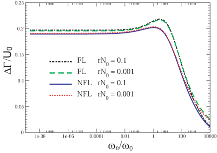
Figure 3: Vertex corrections for forward scattering in $D=2$ in the FL and NFL cases for several values of the curvature $r$.

In Fig. 3 we present the numerical results obtained from Eq.(23) for forward scattering ($\varphi=0$) in the NFL and FL cases for different values of the curvature, $r$. We find that in both cases, ${\Delta\Gamma}$ approaches a finite value in the limit $\omega_{n}\rightarrow 0$, consistent with the findings by Rech et al. Rech et al. (2006), and is almost frequency independent upto a frequency of order $O(\omega_{0})$ where it exhibits a weak maximum before rapidly decreasing at larger frequencies. Moreover, $\Delta\Gamma$ exhibits a very similar functional form for the NFL and FL cases exhibiting only a small quantitative difference in the overall scale. Note that in both cases, ${\Delta\Gamma}$ varies only weakly with curvature $r$. In order to understand the similar frequency dependence in the NFL and FL cases, we evaluate Eq.(27) analytically. Since $\Delta\Gamma$ depends only weakly on $r$, we set for simplicity $r=0$. Moreover, since the poles of the Greens functions in Eq.(27) lie in the same half of the complex plane for $\varphi=0$, it is necessary to introduce a finite upper cut-off, $q_{max}$, in the momentum integration in order to obtain a non-zero result for $\Delta\Gamma$. Note that the numerical evaluation of Eq.(23), in which the momentum decoupling, Eq.(12), is not employed, yields a finite value for $\Delta\Gamma$ even in the limit $q_{max}\rightarrow\infty$ due to the branch cut contribution coming from $\chi$ Rech et al. (2006). After performing the momentum integration in Eq.(27) and rescaling $\hat{\nu}_{m}\equiv\frac{\nu_{m}}{v_{F}q_{max}}$ one obtains

$$\frac{{\Delta\Gamma}}{U_{0}}=-\frac{2I_{s}}{9\pi}\left(\frac{\omega_{0}}{v_{F}q_{max}}\right)^{1/3}\int_{-\infty}^{\infty}\frac{d\hat{\nu}_{m}}{1+Z^{2}(\hat{\nu}_{m})}\frac{1}{|\hat{\nu}_{m}-{\hat{\omega}_{n}}|^{1/3}}\ .$$ (28)

In the limit ${\hat{\omega}}_{0}=\omega_{0}/v_{F}q_{max}\ll 1$ considered here (for the numerical results in Fig. 3, one has ${\hat{\omega}}_{0}=2\times 10^{-4}$), one obtains $|\hat{\nu}_{m}+{\hat{\omega}}_{0}^{1/3}\hat{\nu}_{m}^{2/3}|\approx|\hat{\nu}_{m}|$ for $\hat{\nu}_{m}\gg{\hat{\omega}}_{0}$, implying that the term $[1+Z^{2}(\hat{\nu}_{m})]^{-1}$ in the integrand of Eq.(28), is approximately the same for the FL and NFL cases, thus explaining the small quantitative differences between these two cases.

IV.2 Backward scattering

We begin by discussing the FL case, for which the analytical derivation of ${\Delta\Gamma}$, starting from Eq.(27), is presented in Appendix A. Since the final expression for ${\Delta\Gamma}$ given in Eq.(55) is rather cumbersome, we fill focus here on two limiting cases. In the low-frequency limit $\omega_{n}\ll\omega_{r}$, the asymptotic behavior of ${\Delta\Gamma}$ is given by

$$\frac{{\Delta\Gamma}}{U_{0}}=\frac{3}{16\pi}\frac{1}{N_{0}r}\ln\left(\frac{\omega_{n}}{\omega_{0}}\right)-O\left(\omega_{n}^{1/3}\right)$$ (29)

while for $\omega_{n}\gg\omega_{r}$, one obtains

$$\frac{{\Delta\Gamma}}{U_{0}}= 2\left(\frac{\omega_{n}}{\omega_{0}}\right)^{-1/3}-\sqrt{\frac{3}{2}}z^{-1/2}\left(\frac{\omega_{n}}{\omega_{0}}\right)^{-1/2}$$

$$\quad-O\left[\frac{\ln(\omega_{n})}{\omega_{n}}\right]$$ (30)

with

$$z=\frac{\sqrt{3}}{4\pi}\frac{1}{rN_{0}}\ .$$ (31)

Here, $\omega_{r}=z^{-3}\omega_{0}\sim r^{3}$ is the crossover frequency between the high and low frequency limits which strongly varies with the curvature of the Fermi surface. In the low-frequency limit, ${\Delta\Gamma}$ exhibits a logarithmic divergence whose prefactor depends inversely on the local curvature, $r$. In contrast, in the high frequency limit, the leading order frequency dependence of ${\Delta\Gamma}$ is algebraic with an $r$-independent prefactor.

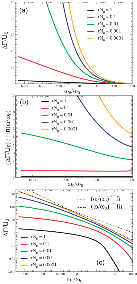
Figure 4: Backward scattering in 2D for the FL case: (a) $\Delta\Gamma/U_{0}$, (b) $(\Delta\Gamma/U_{0})/|\ln\left(\omega_{n}/\omega_{0}\right)|$, (c) log-log plot of ${\Delta\Gamma}/U_{0}$ with fits to $(\omega_{n}/\omega_{0})^{-1/3}$ (dotted line) and $(\omega_{n}/\omega_{0})^{-1/4}$ (dashed line).

In Fig. 4(a), we present the frequency dependence of $\Delta\Gamma$ for the FL case and backward scattering obtained numerically from Eq.(23) for different values of curvature $r$. In agreement with the analytical results in Eq.(29), we find that ${\Delta\Gamma}$ diverges in the limit $\omega_{n}\rightarrow 0$ and that its overall scale decreases with increasing $r$. In order to extract the functional dependence of ${\Delta\Gamma}$ in the low-frequency limit, we plot in Fig. 4(b) the ratio $R=({\Delta\Gamma}/U_{0})/|\ln(\omega_{n}/\omega_{0})|$. For $rN_{0}=1$ and $0.1$, this ratio is constant in the low-frequency limit, implying a logarithmically diverging ${\Delta\Gamma}$, in agreement with Eq.(29). For $rN_{0}=0.01$, $R$ still possesses a substantial frequency dependence at low frequencies, however, its second derivative, $d^{2}R/d\ln^{2}(\omega)$, is negative, suggesting that $R$ approaches a constant value for $\omega_{n}\rightarrow 0$. However, for $rN_{0}=0.001$ and $0.0001$, we find that $R$ strongly increases with decreasing $\omega_{n}$ upto the smallest frequencies that we can access numerically. The problem in establishing a logarithmic divergence of ${\Delta\Gamma}$ for small values of $rN_{0}$ arises from the fact that this divergence emerges only in the limit $\omega\ll\omega_{r}\sim r^{3}\omega_{0}$. Since $\omega_{r}$ decreases strongly with decreasing curvature $r$, it becomes increasingly difficult to identify the logarithmic divergence over the numerically accessible frequency range. For example, for $rN_{0}=0.0001$, one has $\omega_{r}=3.82\times 10^{-10}\omega_{0}$ which is smaller than the smallest frequencies we can consider. The approach to a logarithmic divergence at low frequencies, however, can be seen by considering a log-log plot of ${\Delta\Gamma}$, as shown in Fig. 4(c). For $rN_{0}=0.0001$ we find that at larger frequencies $\omega_{n}/\omega_{0}\gtrsim 10^{-3}$, ${\Delta\Gamma}$ scales approximately as $\omega_{n}^{-1/3}$ while in the low-frequency range $10^{-9}\gtrsim\omega_{n}/\omega_{0}\gtrsim 10^{-4}$, we have ${\Delta\Gamma}\sim\omega_{n}^{-1/4}$ [see straight lines in Fig. 4(c)]. The decrease in the exponent of the algebraic dependence with decreasing frequency suggests that ${\Delta\Gamma}$ eventually crosses over to a logarithmic form in the limit $\omega_{n}\rightarrow 0$.

In the high-frequency limit, $\omega_{n}\gg\omega_{r}$, the leading frequency dependence is given by ${\Delta\Gamma}\sim\omega_{n}^{-1/3}$ [see Eq.(30)]. There are two reasons why this behavior is not necessarily observed in the numerical results shown in Fig. 4(c). First, ${\Delta\Gamma}\sim\omega_{n}^{-1/3}$ holds only for the case of an infinitely large fermionic band. In contrast, for the numerical evaluation of ${\Delta\Gamma}$, it is necessary to introduce a finite cut off in the frequency ($\omega_{max}$) and momentum ($q_{max}$) integration (with $\omega_{max}=v_{F}q_{max}$) which establishes a finite fermionic bandwidth (we set $\omega_{max}=5000\omega_{0}$ for the results shown in Fig.4). Once $\omega_{n}$ exceeds $\omega_{max}$, ${\Delta\Gamma}$ decrease more rapidly than $\omega_{n}^{-1/3}$. In order to further demonstrate the dependence of ${\Delta\Gamma}$ on the $\omega_{max}$ we present in Fig. 5 the frequency dependence of ${\Delta\Gamma}$ for $rN_{0}=0.001$ and several values of $\omega_{max}$.

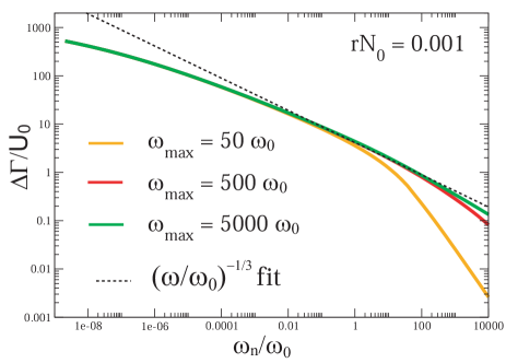
Figure 5: ${\Delta\Gamma}/U_{0}$ in the FL case for backward scattering in $D=2$ and several values of the frequency cut-off, $\omega_{max}=v_{F}q_{max}$ together with a fit to ${\Delta\Gamma}\sim\omega_{n}^{-1/3}$.

As $\omega_{max}$ increases, ${\Delta\Gamma}$ decreases slower and extends its $\omega_{n}^{-1/3}$-behavior towards higher frequencies, as expected from the above discussion. Second, in order to observe ${\Delta\Gamma}\sim\omega_{n}^{-1/3}$, it is necessary for the subleading $\omega_{n}^{-1/2}$-term [see Eq.(30)] to be negligible in comparison to the leading $\omega_{n}^{-1/3}$-term. We find that the frequency, above which the subleading term is negligible, can be much larger than $\omega_{max}$. To quantify this result, consider the frequency $\omega_{\beta}=(3/8z)^{3}\beta^{6}\omega_{0}$ such that for $\omega_{n}>\omega_{\beta}$, the ratio of the subleading to leading frequency term in ${\Delta\Gamma}$ is smaller than $\beta$. Since, $z\sim 1/r$, one immediately finds that for values of $rN_{0}$ of order $O(1)$, $\omega_{\beta}$ exceeds $\omega_{max}$ even for small values of $\beta$. This explains why for values of the curvature such as $rN_{0}=1$ or $rN_{0}=0.1$ [see Fig.4(c)], ${\Delta\Gamma}\sim\omega_{n}^{-1/3}$ is only observed as a crossover behavior between the low-frequency logarithmic divergence and the more rapid decrease at high frequencies. As $rN_{0}$ decreases, the frequency range over which ${\Delta\Gamma}\sim\omega_{n}^{-1/3}$ is observed increase because both $\omega_{r}$ and $\omega_{\beta}$ decrease, while $\omega_{max}$ remains unchanged.

For the NFL case, the derivation of ${\Delta\Gamma}$ is presented in Appendix A. For $\omega_{n}<\omega_{0}$ one obtains [see Eq.(51)]

$${\Delta\Gamma}=G(r)\ln\left(\frac{\omega_{0}}{\omega_{n}}\right).$$ (32)

where the full form of $G(r)$ is given in Eq.(52) (the logarithmic frequency dependence is similar to the one obtained in the context of a $U(1)$ gauge theory Alt95 ). In the NFL case, there exists no crossover scale (such as $\omega_{r}$ in the FL case) to an algebraic dependence of ${\Delta\Gamma}$ below $\omega_{0}$. However, since the upper bound for NFL behavior in the fermionic propagator is set by $\omega_{0}$, one finds that for $\omega_{n}\gg\omega_{0}$, ${\Delta\Gamma}$ exhibits the same frequency dependence as was obtained for the FL case [see Eq.(30)]. Hence, in the NFL case, the crossover scale from a logarithmic to an algebraic dependence of ${\Delta\Gamma}$ is set by the larger one of $\omega_{0}$ and $\omega_{r}$.

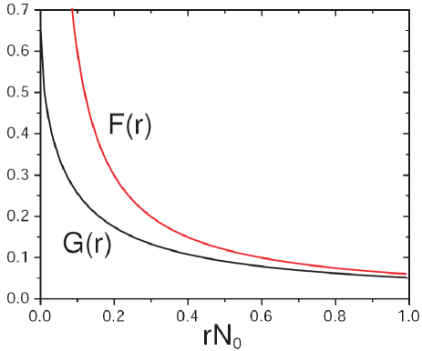
Figure 6: $G(r)$ and $F(r)$ as a function of $rN_{0}$.

In Fig. 6 we present the prefactors of the logarithmic frequency dependence for the NFL and FL cases, $G(r)$ and $F(r)=3/(16\pi rN_{0})$, respectively, as a function of curvature. In both cases, the overall scale of the logarithmic divergence, rapidly decreases with increasing $r$. Since for all $r$, $F(r)>G(r)$, we conclude that the inclusion of the fermionic self-energy [see Eq.(14)] which renders the fermionic Greens function non-Fermi-liquid like, leads to a suppression of the overall scale of the vertex correction, ${\Delta\Gamma}$. Moreover, in the limit of vanishing curvature, $r\rightarrow 0$, one has $G(r)\rightarrow 2/3$. Hence, the prefactor of the log-divergence is finite, in contrast to the FL case where $F(r)$ diverges as $\sim r^{-1}$. In the opposite limit, $r\rightarrow\infty$, one finds to leading order $G(r)\approx 3/(16\pi rN_{0})$, and hence $G(r)$ approaches $F(r)$ asymptotically.

In Fig. 7(a), we present the frequency dependence of $\Delta\Gamma$ for backward scattering ($\varphi=\pi$) as obtained numerically from Eq.(23) for the NFL case and different values of curvature $r$.

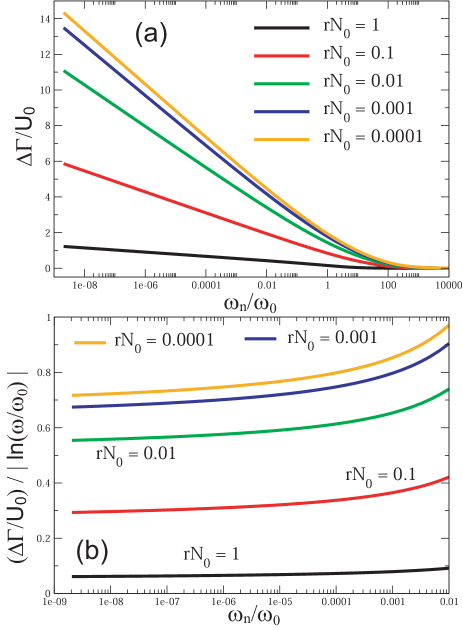
Figure 7: Backward scattering in $D=2$ for the NFL case: (a) $\Delta\Gamma/U_{0}$, (b) $(\Delta\Gamma/U_{0})/|\ln\left(\omega_{n}/\omega_{0}\right)|$.

In agreement with our analytical results in Eq.(32) we find that ${\Delta\Gamma}$ diverges logarithmically for $\omega_{n}\rightarrow 0$. This conclusion is supported by Fig. 7(b), where we again plot the ratio $({\Delta\Gamma}/U_{0})/|\ln(\omega_{n}/\omega_{0})|$ which approaches a constant value for $\omega_{n}\rightarrow 0$. Moreover, our numerical results confirm that (a) in the limit of vanishing curvature, the prefactor of the logarithmic divergence approaches a finite value, and (b) that the overall scale of the vertex corrections is suppressed with increasing curvature. Finally, a comparison of the results for the FL case in Fig. 4(a) with those of the NFL case in Fig. 7(a) support our earlier conclusion that the NFL nature of the fermionic Greens function suppresses the overall scale of ${\Delta\Gamma}$.

IV.3 Angular dependence of ${\Delta\Gamma}$

In Fig. 8, we present ${\Delta\Gamma}$ for $\omega_{n}=2\times 10^{-9}\omega_{0}$ as a function of the scattering angle, $\varphi$ in the FL and NFL cases.

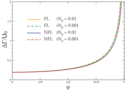
Figure 8: ${\Delta\Gamma}/U_{0}$ for $\omega_{n}=2\times 10^{-9}\omega_{0}$ as a function of the scattering angle, $\varphi$, for the NFL and FL cases in $D=2$ and several values of $r$.

In both cases, ${\Delta\Gamma}$ increases monotonically with increasing $\varphi$. Moreover, ${\Delta\Gamma}$ is practically frequency independent upto frequencies of order $\omega_{0}$ over a wide range of scattering angles (not shown). Only in the immediate vicinity of backward scattering ($\varphi\approx\pi$) does the frequency dependence of ${\Delta\Gamma}$ depend very sensitively on the scattering angle $\varphi$, as we discuss next.

In order to gain analytical insight into the form of ${\Delta\Gamma}$ in the vicinity of backward scattering, we consider the case $r=0$ for which a full analytical expression of ${\Delta\Gamma}$ can be obtained (the derivation is similar to the one discussed in Appendix A). We begin by discussing the FL case, where in the low frequency limit, $\omega_{n}\rightarrow 0$, one obtains

$$\frac{{\Delta\Gamma}}{U_{0}}=\frac{3\pi}{4}\sqrt{\frac{\alpha}{\phi}}\ ,$$ (33)

with $\phi=\pi-\varphi$ such that $\phi=0$ corresponds to backward scattering. In the high-frequency limit, $\omega_{n}\gg\omega^{FL}_{\phi}$, we have

$$\frac{{\Delta\Gamma}}{U_{0}}=2\left(\frac{\omega_{n}}{\omega_{0}}\right)^{-1/3}\ ,$$ (34)

with the crossover scale being set by

$$\omega_{\phi}^{FL}=z^{-3/2}\omega_{0}=\left(\frac{2\phi}{3\alpha}\right)^{3/2}\omega_{0}\ ,$$ (35)

which decreases with $\phi$. We thus find that a non-zero angle $\phi$ eliminates the low-frequency logarithmic divergence of ${\Delta\Gamma}$ [see Eq.(29)] and leads to a constant value of ${\Delta\Gamma}$ for $\omega_{n}\rightarrow 0$. In contrast, the high-frequency form of ${\Delta\Gamma}$ remains unchanged from that for backward scattering ($\phi=0$) shown in Eq.(30).

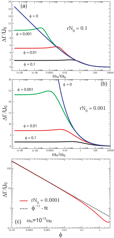
Figure 9: ${\Delta\Gamma}/U_{0}$ in $D=2$ as a function of $\omega_{n}$ for the FL case and several values of $\phi$: (a) $rN_{0}=0.1$, and (b) $rN_{0}=0.001$. (c) ${\Delta\Gamma}/U_{0}$ as a function of $\phi$ for $rN_{0}=0.0001$ and $\omega_{n}=10^{-13}\omega_{0}$.

In Figs. 9(a) and (b) we present the frequency dependence of ${\Delta\Gamma}$ for the FL case, as obtained from the numerical evaluation of Eq.(23), for several values of $\phi$ and curvature $r$. For comparison, we have also included the results for backward scattering, corresponding to $\phi=0$. In agreement with the analytical results presented above, we find that the logarithmic divergence is eliminated by a non-zero $\phi$, and that ${\Delta\Gamma}$ approaches a constant value for $\omega_{n}\rightarrow 0$. In addition, for frequencies above some crossover scale, ${\Delta\Gamma}$ for $\phi\not=0$ exhibits the same frequency dependence as that for $\phi=0$, as expected from Eq.(34). It is, in general, difficult to estimate a quantitative value for the crossover scale from the numerical data presented in Figs. 9(a) and (b), and to compare them directly with the analytically obtained result. However, taking, for example, the maxima in ${\Delta\Gamma}$ as a measure of the crossover scale, we find that they scale as $\sim\phi^{3/2}$, in agreement with the analytical result given in Eq.(35). Finally, in Fig. 9(c) we present ${\Delta\Gamma}$ for vanishing frequency ($\omega_{n}=10^{-13}\omega_{0}$) and small $rN_{0}=0.0001$, as a function of deviation from backward scattering, $\phi$. We find that ${\Delta\Gamma}$ scales as $1/\sqrt{\phi}$ [see dotted line in Fig. 9(c)], in agreement wit the analytical result presented in Eq.(33).

We next turn to the NFL case, where one obtains for $z\gg 1$ and in the limit $\omega_{n}\rightarrow 0$

$$\frac{{\Delta\Gamma}}{U_{0}}=2\ln\left(\frac{3\alpha}{2\phi}\right),$$ (36)

in qualitative agreement with the result obtained by Kim and Millis Kim:2003 . In the intermediate frequency regime, $\omega^{NFL}_{\phi}\ll\omega_{n}\ll\omega_{0}$, one has to leading order

$$\frac{{\Delta\Gamma}}{U_{0}}=\frac{2}{3}\ln\left(\frac{\omega_{n}}{\omega_{0}}\right)\ .$$ (37)

Here, the crossover scale is set by

$$\omega^{NFL}_{\phi}=\left(\frac{2\phi}{3\alpha}\right)^{3}\omega_{0}\ .$$ (38)

For $\omega_{n}\gg\omega_{0}$, ${\Delta\Gamma}$ again takes the FL form given in Eq.(30). Similar to the FL case, we find that a non-zero $\phi$ eliminates the logarithmic divergence for $\omega_{n}\rightarrow 0$. In addition, there exists an intermediate frequency range ($\omega^{NFL}_{\phi}\ll\omega_{n}\ll\omega_{0}$) in which ${\Delta\Gamma}$ exhibits a logarithmic frequency dependence, in contrast to the FL case. Note that it was argued in Ref. Kim:2003 that the logarithmic dependence of ${\Delta\Gamma}$ on $\phi$ is responsible for the anomalies observed in the residual resistivity of ${\rm Sr_{3}Ru_{2}O_{7}}$ at the metamagnetic transition.

In Figs. 10(a) and(b) we present the frequency dependence of ${\Delta\Gamma}$ for the NFL case obtained from the numerical evaluation of Eq.(23), for several values of $\phi$ and $r$.

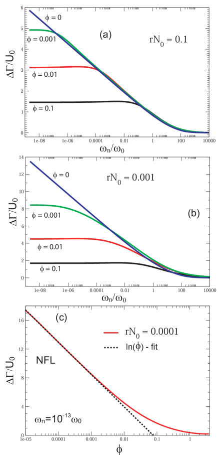
Figure 10: ${\Delta\Gamma}/U_{0}$ in $D=2$ as a function of $\omega_{n}$ for the NFL case and several values of $\phi$: (a) $rN_{0}=0.1$, and (b) $rN_{0}=0.001$. (c) ${\Delta\Gamma}/U_{0}$ as a function of $\phi$ for $rN_{0}=0.0001$ and $\omega_{n}=10^{-13}\omega_{0}$.

In agreement with our analytical results we find that for non-zero $\phi$, ${\Delta\Gamma}$ saturates to a finite value in the limit $\omega_{n}\rightarrow 0$, and that the crossover scale (below which ${\Delta\Gamma}$ becomes approximately constant) increases with $\phi$. Above the crossover scale, the form of ${\Delta\Gamma}$ for backward scattering ($\phi=0$) and away from backward scattering ($\phi\not=0$) are practically identical. For small values of $rN_{0}$, and in the limit $\phi\rightarrow 0$, we find that ${\Delta\Gamma}$ scales as $\sim\ln{\phi}$ [see dotted line in Fig. 10(c)], in agreement wit the analytical result presented in Eq.(36). Moreover, a comparison of Figs. 9 and 10 confirms two important analytical results. First, the limiting value of ${\Delta\Gamma}$ for $\omega_{n}\rightarrow 0$ is smaller in the NFL than in the FL case [see Eqs.(33) and (36)]. Second, for a given $\phi$, the crossover scale is smaller for the NFL case than it is for the FL case, i.e., $\omega^{NFL}_{\phi}\ll\omega^{FL}_{\phi}$. By comparing the result for $\phi=0.001$ in Figs. 9(a) and (b) [and similarly, in Figs. 10(a) and (b)] we note that in both cases the crossover scale moves to lower frequencies with increasing $r$.

V Vertex Corrections in $D=3$

Since the higher dimensionality leads to a weaker deviation of the fermionic propagator from Fermi-liquid behavior in $D=3$ than in $D=2$ (see Sec.II), we expect a concurrent weaker renormalization of the scattering amplitude in $D=3$ as well. For the numerical results presented below, we set $\gamma=0.1$, $I_{s}=3$, and give $rN_{0}$ in units of $[\frac{\pi}{k_{F}}\left(\frac{\Lambda}{k_{F}}\right)^{3}]^{-1}$, while $q_{max}$ and $\omega_{max}$ are given in units of $q_{0}\gamma e^{1/\gamma}$ and $\omega_{0}\gamma e^{1/\gamma}$, respectively.

V.1 Forward scattering

The frequency dependence of ${\Delta\Gamma}$ for forward scattering, obtained from the numerical evaluation of Eq.(24) is shown in Figs. 11(a) and (b), for the FL and NFL cases, respectively (similar to our results in $D=2$, we note that the non-zero contribution to ${\Delta\Gamma}$ for forward scattering obtained from the numerical evaluation arises from the branch cut in $\chi$ and the finite cut-off in the momentum integration).

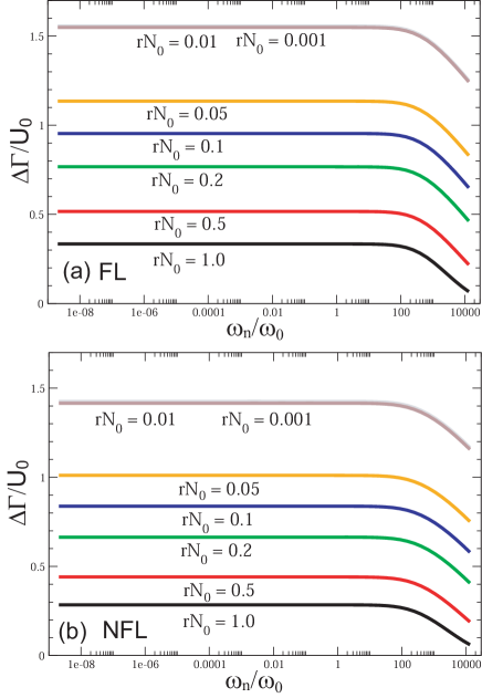
Figure 11: Frequency dependence of ${\Delta\Gamma}/U_{0}$ in $D=3$ for forward scattering and several values of $rN_{0}$: (a) the FL case, and (b) the NFL case (with $\omega_{max}=q_{max}=100$).

In both cases, ${\Delta\Gamma}$ is practically frequency independent for frequencies below $\omega_{0}$, and hence approaches a constant value in the limit $\omega_{n}\rightarrow 0$. We note, however, that the overall scale of ${\Delta\Gamma}$ increases with decreasing $r$, upto a value, $r_{c}$, below which ${\Delta\Gamma}$ becomes independent of $r$ [for example, ${\Delta\Gamma}$ for $rN_{0}=0.01$ and $0.001$ are practically indistinguishable in Figs. 11(a) and (b).] We find from an analytical analysis of Eq.(24) that $r_{c}N_{0}=1/q_{max}$ where $q_{max}$ is the upper cut-off in the momentum integration of Eq.(24). This result is in agreement with our numerical analysis which is summarized in Fig. 12 where we present ${\Delta\Gamma}$ at $\omega_{n}=2\times 10^{-9}\omega_{0}$ as a function of $rN_{0}$ for several $q_{max}$.

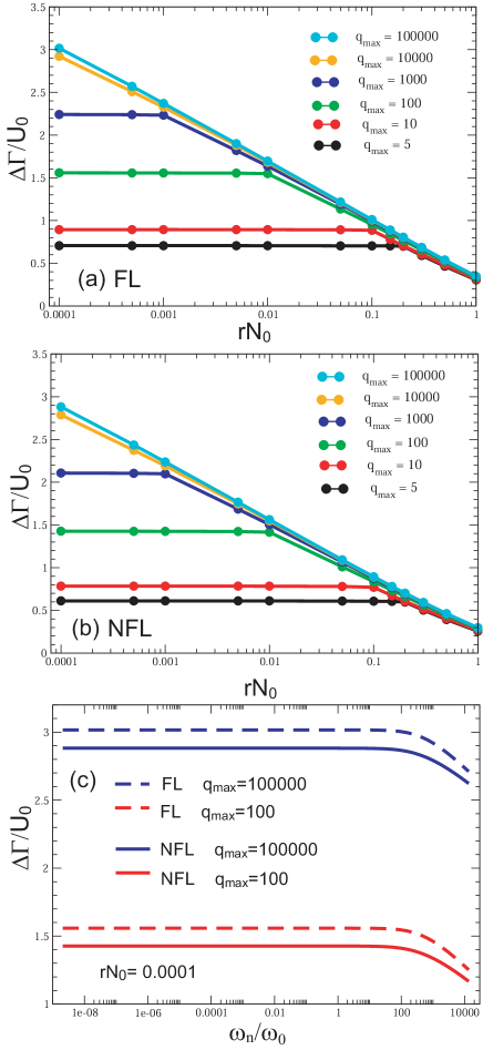
Figure 12: ${\Delta\Gamma}/U_{0}$ for $\omega_{n}=2\times 10^{-9}$ and forward scattering in $D=3$ as a function of $rN_{0}$: (a) the FL case, and (b) the NFL case. (c) Frequency dependence of ${\Delta\Gamma}/U_{0}$ for $rN_{0}=0.0001$ and several values of $q_{max}$.

As follows from Figs. 12(a) and (b), one has ${\Delta\Gamma}\sim\ln(r)$ down to $r_{c}$ below which ${\Delta\Gamma}$ becomes independent of $r$. In order to investigate whether the functional form of the frequency dependence of ${\Delta\Gamma}$ changes between $r<r_{c}$ and $r>r_{c}$, we present in Fig. 12(c) ${\Delta\Gamma}$ as a function of frequency for $rN_{0}=0.0001$ and different values of $q_{max}$. For $q_{max}=100$, one has $r<r_{c}$, while $r>r_{c}$ for $q_{max}=10^{5}$. We find not only that the functional form of ${\Delta\Gamma}$ is practically independent of whether $r$ is smaller or larger than $r_{c}$, but also that the crossover frequency below which ${\Delta\Gamma}$ becomes frequency independent does not change with $r$ or $q_{max}$. This result is in apparent contradiction to the findings of Miyake et al. Miyake:2001 who argued that in the FL case, ${\Delta\Gamma}$ diverges logarithmically for $\omega_{n}\rightarrow 0$. At present, the origin for this discrepancy is unclear. Our result, however, is consistent with the finding that in $D=2$, ${\Delta\Gamma}$ also approaches a finite value for $\omega_{n}\rightarrow 0$, since, in general, one would expect that with increasing dimensionality of the system, fluctuation corrections become weaker, and that as a result, the functional dependence of ${\Delta\Gamma}$ on $\omega_{n}$ should not become stronger in the low frequency limit.

V.2 Backward scattering

In order to gain analytical insight into the functional form of ${\Delta\Gamma}$ for backward scattering in $D=3$, we again start from Eq.(27). In the FL case and in the limit $\omega_{n}\rightarrow 0$, one finds to leading order

$$\frac{{\Delta\Gamma}}{U_{0}}=9\pi^{2}\gamma\left[F\left(x\right)-\frac{\sqrt{2}}{3\rho^{1/2}}\sqrt{\frac{\omega_{n}}{\omega_{0}}}+\frac{2}{3\sqrt{3}\rho^{2/3}}\left(\frac{\omega_{n}}{\omega_{0}}\right)^{2/3}\right]$$ (39)

where $\rho=\lambda^{2}r^{3}/(\langle v_{F}\rangle^{2}\omega_{0})$, $x=\left(\rho^{-1}\omega_{max}/\omega_{0}\right)^{1/3}$, $\omega_{max}$ is the upper cut-off in frequency, and $F(x)$ is a universal function of the upper cut-off, which scales as $F(x)\approx\ln^{2}(x)/(2\pi)$ for $x\to\infty$, i.e. $r\to 0$. In the NFL case we obtain to leading order

$$\frac{{\Delta\Gamma}}{U_{0}}=\frac{3}{2}\left[F\left(x\right)-\frac{\sqrt{2}\pi}{\rho^{1/2}}\sqrt{\left(\frac{\omega_{n}}{\omega_{0}}\right)\ln{\left(\frac{\omega_{0}}{\omega_{n}}\right)}}\right]$$ (40)

with $F(x)$ given above. Thus, the zero frequency limit of ${\Delta\Gamma}$ for both the FL and NFL cases is finite, though it diverges with vanishing curvature $r$ as ${\Delta\Gamma}\sim\ln^{2}(r)$.

In Figs. 13 and 14 we present ${\Delta\Gamma}$ in the FL and NFL cases, respectively, for backward scattering ($\varphi=\pi$), as obtained from the numerical evaluation of Eq.(24).

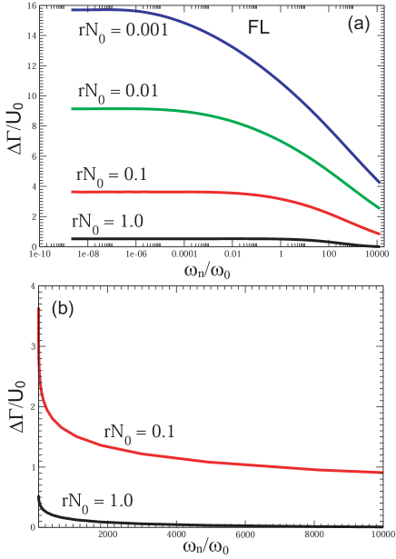
Figure 13: ${\Delta\Gamma}/U_{0}$ in $D=3$ for backward scattering in the FL case for different values of $rN_{0}$: (a) linear-log plot, (b) same results as in (a) but on a linear-linear plot. We set $\omega_{max}=q_{max}=10$.

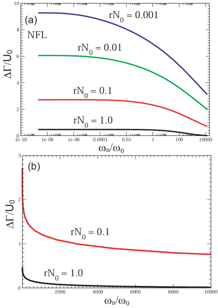
Figure 14: ${\Delta\Gamma}/U_{0}$ in $D=3$ for backward scattering in the NFL case for different values of $rN_{0}$: (a) linear-log plot, (b) same results as in (a) but on a linear-linear plot. We set $\omega_{max}=q_{max}=10$.

In agreement with the analytical results, we find that in both cases, ${\Delta\Gamma}$ approaches a constant value as $\omega_{n}\rightarrow 0$, in contrast to the logarithmic divergence found in $D=2$. Moreover, our numerical results show that ${\Delta\Gamma}$ at the lowest frequency scales as $\sim\ln^{2}(r)$ (in contrast to $\sim\ln(r)$ for forward scattering), and that the leading frequency correction in the FL case is given by $\sim\sqrt{\omega_{n}}$, in agreement with our analytical findings.

V.3 Angular dependence of ${\Delta\Gamma}$

In Fig. 15, we present ${\Delta\Gamma}$ for $\omega_{n}=2\times 10^{-9}\omega_{0}$ as a function of scattering angle $\varphi$ in the FL and NFL cases for several values of $r$.

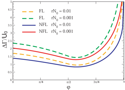
Figure 15: ${\Delta\Gamma}/U_{0}$ for $\omega_{n}=2\times 10^{-9}\omega_{0}$ as a function of scattering angle $\varphi$ in $D=3$ for the NFL and FL cases and several values of $rN_{0}$. We set $\omega_{max}=q_{max}=10^{4}$.

In both cases, ${\Delta\Gamma}$ first decreases with increasing $\varphi$, exhibiting a minimum around $\varphi\approx 0.578\pi$, and then increases sharply as $\varphi$ approaches $\pi$. Similar to the case in $D=2$, we find that ${\Delta\Gamma}$ is practically frequency independent upto frequencies of order $\omega_{0}$ over a wide range of scattering angles. Only in the immediate vicinity of backward scattering ($\varphi\approx\pi$) does the frequency dependence of ${\Delta\Gamma}$ depend very sensitively on the scattering angle $\varphi$. A comparison of Fig. 8 with Fig. 15 show that the dependence of ${\Delta\Gamma}$ on curvature $r$ is significantly stronger in $D=3$ that it is in $D=3$, in agreement with the above analytical results.

VI Higher Order Vertex Corrections

We next discuss the form of higher order vertex corrections, such as the one shown in Fig. 2 (c). It turns out that the low-frequency form of the higher order vertex corrections is entirely determined by that of the lowest order vertex correction, $\Delta\Gamma^{(1)}\equiv{\Delta\Gamma}$ discussed in the previous sections. In what follows, we consider the case of vanishing curvature, where the segments between wavy lines of the higher order (ladder) vertex corrections decouple, and the infinite series of ladder vertex corrections can be summed up.

To demonstrate this, we first consider the case of backward scattering in $D=2$ for the NFL case, where in the low-frequency limit, we found for the lowest order vertex correction ${\Delta\Gamma}^{(1)}={\Delta\Gamma}=2/3\ln(\omega_{0}/\omega_{n})$ [see Eq.(32) for $r=0$]. It then immediately follows that the leading frequency dependence of the $m^{\prime}th$ order vertex correction in the limit $\omega_{n}\rightarrow 0$ is given by

$$\Delta\Gamma^{(m)}=\frac{1}{m!}\left[\frac{2}{3}\ln\left(\frac{\omega_{0}}{\omega_{n}}\right)\right]^{m}$$ (41)

Summing up the entire series of ladder vertex corrections (including the bare vertex) yields for the renormalized scattering vertex for backward scattering

$$U=U_{0}\left(\frac{\omega_{n}}{\omega_{0}}\right)^{-2/3}$$ (42)

Performing the analytical continuation to real frequencies, one obtains

$$U=U_{0}\left(\frac{\omega}{\omega_{0}}\right)^{-2/3}e^{\sigma i\pi/3}$$ (43)

where the choice of the branch in the complex plane ($\sigma=\pm$) is determined by requirement that the LDOS, renormalized by the scattering off the impurity, be positive. For a particle-hole symmetric band structure, we find that this requirement is met by using $\sigma=-{\rm sgn}(U_{0})$. We thus find an algebraic frequency divergence of the full vertex in the low frequency limit, similar to the result obtained by Altshuler et al. Alt95 in the context of a $U(1)$ gauge theory. For zero frequency, it was shown by Kim and Millis Kim:2003 that the same summation of ladder diagrams in $D=2$ for the NFL case leads to similar algebraic dependence of ${\Delta\Gamma}$ on the deviation from backward scattering, $\phi$.

As a second example for the form of the higher order ladder diagrams, we consider the case where the lowest order vertex correction, ${\Delta\Gamma}^{(1)}$, approaches a constant value in the limit $\omega_{n}\rightarrow 0$, i.e., ${\Delta\Gamma}^{(1)}/U_{0}=A$. In the same limit, the $m^{\prime}th$ order vertex correction is given by

$$\frac{\Delta\Gamma^{(m)}}{U_{0}}=A^{m}\ .$$ (44)

Summing up the entire series of ladder vertex corrections (including the bare vertex) yields for the renormalized scattering vertex for backward scattering

$$U=U_{0}\frac{1}{1-A}$$ (45)

As a result, we find that even for those cases where the lowest order vertex correction does not diverge in the limit $\omega_{n}\rightarrow 0$, the full scattering vertex can be enhanced, or even diverge, depending on the zero-frequency limit of ${\Delta\Gamma}^{(1)}$. Finally, note that the (crossing) vertex correction diagrams of the type shown in Fig. 2 (d) are expected to not qualitatively modify the results given in Eq.(43) and Eq.(45), [Kim:2003, ].

VII Conclusions

Table 1: Summary of the leading frequency dependence of ${\Delta\Gamma}$ for backward scattering in the limit $\omega_{n}\rightarrow 0$. All quantities are defined in the main text. The function $G$ is given by Eq.(52) and shown in Fig. 6. As stated in the text, after Eq.(39), $F(x)$ is a universal function, which scales as $F(x)\approx\ln^{2}(x)/(2\pi)$ for $x\to\infty$, where $x=r^{-1}(v_{F}^{2}\Omega_{c}/\lambda^{2})^{1/3}$. For forward scattering we find that both in $D=2$ and $3$ the lowest order vertex corrections do not diverge as $\omega_{n}\to 0$.

	Fermi Liquid	Non-Fermi liquid
$D=2$	ΔΓU0 = 316π1rN0ln(ωnω0)	ΔΓU0 ≈G(r)ln(ω0ωn)
$D=3$	ΔΓU0 = 9 π^2 γ[ F( x )-23 ρ1/2 ωnω0 ]	ΔΓU0 = 32 [ F(x ) -2πρ1/2 (ωnω0)ln(ω0ωn) ]

In summary, we have studied the renormalization of a non-magnetic impurity’s scattering potential due to the presence of a massless collective spin mode at a ferromagnetic quantum critical point. For the case of a single, isolated impurity (corresponding to the limit of a vanishing impurity density), we computed the lowest order vertex corrections in two- and three-dimensional systems, for arbitrary scattering angle, frequency and curvature. We showed that only for backward scattering, $\varphi=\pi$, in $D=2$ does the lowest order vertex correction diverge logarithmically in the limit $\omega_{n}\rightarrow 0$ (a summary of these results is shown in Table 1). A similar result (for the NFL case) was obtained in the context of a $U(1)$ gauge theory by Altshuler et al. Alt95 . For $\varphi\not=\pi$ in $D=2$, and for all $\varphi$ in $D=3$, we find that the vertex corrections both for the NFL and FL cases approach a finite (albeit possibly large) value in the low-frequency limit. In particular, in the vicinity of backward scattering in $D=2$, we find that the logarithmic frequency divergence in ${\Delta\Gamma}$ is cut by a non-zero deviation from backward scattering, $\phi$, with ${\Delta\Gamma}\sim 1/\sqrt{\phi}$ for the FL case, and ${\Delta\Gamma}\sim\ln(\phi)$ in the NFL case. The latter result is in qualitative agreement with that obtained by Kim and Millis Kim:2003 . Moreover, for the NFL case and forward scattering in $D=2$, our finding of a finite ${\Delta\Gamma}$ in the limit $\omega_{n}\rightarrow 0$ agrees with that by Rech et al. Rech et al. (2006). However, our results are in disagreement with those of Miyake et al.Miyake:2001 who for the FL case reported a logarithmic divergence in frequency of ${\Delta\Gamma}$ for forward scattering in $D=3$. The origin of this discrepancy is presently unclear.

We also showed that the overall scale of vertex corrections is weaker in the NFL than in the FL case, implying that the NFL nature of the fermionic degrees of freedom diminish the vertex corrections. Furthermore, we demonstrated that vertex corrections for backward scattering are strongly suppressed with increasing curvature of the fermionic bands; the qualitative nature of this suppression, however, is different in the NFL and FL cases. Moreover, ${\Delta\Gamma}$ exhibits in general a stronger dependence on $r$ in $D=3$ than in $D=2$. In particular, for forward scattering, we find that in $D=2$, ${\Delta\Gamma}$ in the low-frequency limit is practically independent of the curvature, $r$, but that in $D=3$, ${\Delta\Gamma}$ depends logarithmically on $r$ down to $r_{c}N_{0}=1/q_{max}$ below which it becomes independent of $r$. We explicitly computed the full angular dependence of the vertex correction, and showed that they vary only weakly over a large range of scattering angles and frequencies, but are strongly enhanced in the vicinity of backward scattering. Finally, we considered higher order ladder vertex corrections, and showed that their zero-frequency limit, for $r\to 0$, is solely determined by that of the lowest order vertex correction. As a result, it is possible to sum an infinite series of ladder diagrams. We showed that for backward scattering in $D=2$, this summation changes the logarithmic frequency dependence of the lowest order vertex correction into an algebraic frequency dependence of the fully renormalized scattering vertex. For zero frequency, it was shown by Kim and Millis Kim:2003 that a summation of ladder diagrams in $D=2$ for the NFL case leads to similar algebraic dependence of ${\Delta\Gamma}$ on the deviation from backward scattering.

The question naturally arises whether the combined angular and frequency dependence of the vertex corrections discussed above are experimentally measurable, for example, via a combination of frequency dependent and local measurements. For example, by using several impurities in a well-defined spatial geometry (which could predominantly probe vertex corrections for certain scattering angles), scanning tunneling spectroscopy experiments could provide insight into the combined angular and frequency dependence of vertex corrections via measurements of the local density of states. Moreover, since the resistivity of a material is predominantly determined by backscattering, the frequency dependence of ${\Delta\Gamma}$ for backscattering might be experimentally detectable in the optical conductivity Belitz et al. (2000). A theoretical investigation of these questions is reserved for future studies. We note, however, that the combination of theoretical and experimental results on the form of the LDOS and the optical conductivity will provide important insight into the nature of vertex corrections in particular, and into the interplay of quantum fluctuations and disorder in general.

VIII Acknowledgments

We thank A. Chubukov, D. Maslov, A. Millis, K. Miyake, and G. Schwiete for helpful discussions. D.K.M. acknowledges financial support by the National Science Foundation under Grant No. DMR-0513415 and the U.S. Department of Energy under Award No. DE-FG02-05ER46225.

Appendix A Derivation of ${\Delta\Gamma}$ in $D=2$ for backward scattering

The analytical derivation of ${\Delta\Gamma}$ starts from Eq.(27). Performing the integration over $q_{\parallel}$ yields

$$\frac{{\Delta\Gamma}}{U_{0}} = -\frac{3g^{2}\chi_{0}}{(2\pi)^{3}}\frac{\pi}{v_{F}}\int_{-\infty}^{\infty}d\nu\int_{-\infty}^{\infty}dq_{\perp}\frac{1}{q^{2}_{\perp}+\frac{\lambda|\omega_{n}-\nu|}{v_{F}|q_{\perp}|}}$$ (46)

$$\times\frac{1}{F(|\nu|)+irq^{2}_{\perp}{\rm sign}(\nu)}$$

where $F(|\nu|)=|\nu|$ for the FL case and $F(|\nu|)=|\nu|+\omega_{0}^{1/3}|\nu|^{2/3}$ for the NFL case. While it is possible to analytically perform the integrations over $q_{\perp}$ and $\nu$ in Eq.(46), it turns out that a better analytical understanding of ${\Delta\Gamma}$ can be obtained by eliminating the frequency $\omega_{n}$ from the integrand and reintroducing it as a lower cut-off in the frequency integration. We explicitly checked (analytically and numerically) that the resulting leading order frequency dependence of ${\Delta\Gamma}$ as discussed above is the same in both methods. We then obtain (dropping the subscript of $q_{\perp}$)

$$\frac{{\Delta\Gamma}}{U_{0}} = -\frac{12g^{2}\chi_{0}}{(2\pi)^{3}}\frac{\pi}{v_{F}}\int_{\omega_{n}}^{\infty}d\nu\int_{0}^{\infty}dq\frac{q}{q^{3}+\frac{\lambda\nu}{v_{F}}}$$ (47)

$$\times\frac{F^{2}(|\nu|)}{F^{2}(|\nu|)+r^{2}q^{4}}\ .$$

Rescaling momenta and frequencies as

$$\hat{\omega}=\frac{\omega}{\omega_{0}};\,\hat{q}=\frac{q}{q_{0}};\,q_{0}=\frac{\omega_{0}}{v_{F}};\,{\hat{F}}=\frac{F}{\omega_{0}}$$ (48)

one obtains

$$\frac{{\Delta\Gamma}}{U_{0}} = -\frac{12g^{2}\chi_{0}}{(2\pi)^{3}}\frac{\pi}{v_{F}}\int_{\omega_{n}}^{\Omega_{\Lambda}}d\nu\int_{0}^{\infty}d{\hat{q}}\frac{{\hat{q}}}{{\hat{q}}^{3}+\beta^{3}{\hat{\nu}}}$$ (49)

$$\times\frac{{\hat{F}}^{2}(|\nu|)}{{\hat{F}}^{2}(|\nu|)+{\hat{r}}^{2}{\hat{q}}^{4}}$$

where

$$\beta\equiv\frac{4}{3}\alpha^{-1};\quad{\hat{r}}\equiv r\frac{q^{2}_{0}}{\omega_{0}}$$ (50)

We next consider the NFL case. Since the upper frequency cut-off for NFL behavior is set by $\omega_{0}$, we can introduce $\omega_{0}$ as a high frequency cut-off in the frequency integration, and use the approximation $F(|\nu|)\approx\omega_{0}^{1/3}|\nu|^{2/3}$ which is valid for $\omega_{n}<\omega_{0}$ (for $\omega_{n}>\omega_{0}$ the fermionic propagator is FL-like, and ${\Delta\Gamma}$ takes the FL form discussed below). We then obtain to leading order in $\omega_{n}/\omega_{0}$

$$\Delta\Gamma(\omega_{n})=G(z)\ln\left(\frac{\omega_{0}}{\omega_{n}}\right)$$ (51)

where $z$ is given in Eq.(31) and

$$G(z) = \frac{\sqrt{3}}{4}\frac{z}{1+z^{6}}\left[1+\frac{8}{3\sqrt{3}}z(z^{4}-1)\right.$$ (52)

$$\quad\left.+\sqrt{2}z^{3/2}(1-z^{3})+\frac{2}{\pi}z^{3}\ln z\right]$$

In contrast, for the FL case, the integration of ${\hat{q}}$ in Eq.(49) yields

$${\Delta\Gamma}(\omega_{n})=-\frac{3}{16\pi}\frac{1}{N_{0}r}\int_{y_{n}}^{\infty}dy\frac{P(y)}{y}$$ (53)

where $y=z^{3}\hat{\nu}$ and

$$P(y)= \frac{1}{1+y^{2}}\left[1+\frac{8}{3\sqrt{3}}y^{1/3}(y^{4/3}-1)\right.$$

$$\left.+\sqrt{2}y^{1/2}(1-y)+\frac{1}{9\pi}y\ln y\right].$$ (54)

Performing the final integral over $y$, one obtains

$${\Delta\Gamma}(\omega_{n})=-\frac{3}{16\pi^{2}}\frac{1}{N_{0}r}R(y_{n})$$ (55)

where

$$R(y_{n})= i\pi-\ln y_{n}+\frac{1}{2}\ln(1+y_{n}^{2})-2\arctan y_{n}\ln y_{n}+\ln\left[\frac{1+\sqrt{2}y_{n}^{1/6}-y_{n}^{1/3}}{-1+\sqrt{2}y_{n}^{1/6}-y_{n}^{1/3}}\right]+\frac{7}{3}\ln\left[\frac{1+\sqrt{2-\sqrt{3}}y_{n}^{1/6}+y_{n}^{1/3}}{1+\sqrt{2+\sqrt{3}}y_{n}^{1/6}+y_{n}^{1/3}}\right]$$

$$+\frac{1}{3}\ln\left[\frac{-1+\sqrt{2-\sqrt{3}}y_{n}^{1/6}-y_{n}^{1/3}}{-1+\sqrt{2+\sqrt{3}}y_{n}^{1/6}-y_{n}^{1/3}}\right]-\frac{i}{18\pi}\left[Li_{2}(iy_{n})-Li_{2}(-iy_{n})\right]$$ (56)

and $Li_{2}$ is the dilogarithm function. Expanding $R(y_{n})$ in the limits $y_{n}\ll 1$ and $y_{n}\gg 1$, one obtains the results for ${\Delta\Gamma}$ presented in Eqs.(29) and (30), respectively.

References

- (1) H. v. Löhneysen, A. Rosch, M. Vojta, and P. Wölfle, Rev. Mod. Phys. 79, 1015 (2007)
- (2) K. Miyake and O. Narikiyo, J. Phys. Soc. Jpn. 71, 867 (2001).
- (3) Y. B. Kim and A. J. Millis Phys. Rev. B 67, 085102 (2003).
- Paul et al. (2005) I. Paul, C. Pépin, B. Narozhny, and D. Maslov, Phys. Rev. Lett. 95, 017206 (2005).
- Belitz et al. (2000) D. Belitz, T. R. Kirkpatrick, R. Narayanan, and T. Vojta, Phys. Rev. Lett. 85, 4602 (2000).
- Perry and et al. (2001) R. S. Perry and et al., Phys. Rev. Lett. 86, 2661 (2001).
- Grigera and et al. (2001) S. Grigera and et al., Science 294, 329 (2001).
- (8) R. Roussev and A. J. Millis, Phys. Rev. B 63, (2001).
- (9) Z. Wang, W. Mao and K. Bedell, Phys. Rev. Lett. 87, 257001 (2001).
- (10) A.V. Chubukov, A. M. Finkel’stein, R. Haslinger, D. K. Morr, Phys. Rev. Lett. 90, 077002 (2003)
- (11) M. Dzero and L.P. Gorkov, Phys. Rev. B 69, 092501 (2004).
- (12) A. V. Chubukov, Phys. Rev. B 71, 245123 (2005).
- (13) P. A. Lee, Phys. Rev. Lett. 63, 680 (1989).
- (14) B. Blok and H. Monien, Phys Rev B 47, 3454 (1993).
- (15) D. V. Khveshchenko, Phys. Rev. B 49, 16893 (1994); D. V. Khveshchenko, Phys. Rev. B 52, 4833 (1995).
- (16) C. Nayak and F. Wilczek, Nucl. Phys. B 430, 534 (1994).
- (17) B. L. Altshuler, L. B. Ioffe, and A. J. Millis, Phys. Rev B 50, 14048 (1994); ibid. Phys. Rev B 52, 5563 (1995).
- Hertz (1976) J. A. Hertz, Phys. Rev. B 14, 1165 (1976).
- Millis (1993) A. J. Millis, Phys. Rev. B 48, 7183 (1993).
- Belitz et al. (1997) D. Belitz, T. R. Kirkpatrick, and T. Vojta, Phys. Rev. B 55, 9452 (1997).
- (21) P. Coleman et al., J. Phys. Cond. Mat. 13, R723 (2001).
- Abanov et al. (2003) A. Abanov, A. V. Chubukov, and J. Schmalian, Adv. Phys. 52, 119 (2003).
- Chubukov and Maslov (2003) A. V. Chubukov and D. L. Maslov, Phys. Rev. B 68, 155113 (2003).
- Belitz et al. (2002) D. Belitz, T. R. Kirkpatrick, and T. Vojta, Phys. Rev. B 65, 165112 (2002).
- Belitz et al. (2005) D. Belitz, T. R. Kirkpatrick, and T. Vojta, Rev. Mod. Phys. 77, 579 (2005).
- Rech et al. (2006) J. Rech, C. Pépin, and A. V. Chubukov, Phys. Rev. B 74, 195126 (2006).
- (27) The result for in , Eq.(23), can be further simplified by performing the integral over analytically via a standard integration over a closed circle in the complex plane. The resulting expression is then evaluated numerically.