The spatial distribution of X-ray selected AGN in the Chandra deep fields: a theoretical perspective

Abstract

We study the spatial distribution of X-ray selected AGN in the framework of hierarchical co-evolution of supermassive black holes (BHs) and their host galaxies and dark matter (DM) haloes. To this end, we have applied the theoretical model developed by Croton et al. (2006), De Lucia & Blaizot (2007) and Marulli et al. (2008) to the output of the Millennium Run and obtained hundreds of realizations of past light-cones from which we have extracted realistic mock AGN catalogues that mimic the Chandra deep fields. We find that the model AGN number counts are in fair agreement with observations both in the soft and in the hard X-ray bands, except at fluxes $\lesssim 10^{-15}$ $\mbox{erg}\,\mbox{cm}^{-2}\,\mbox{s}^{-1}$, where the model systematically overestimates the observations. However, a large fraction of these faint objects is typically excluded from the spectroscopic AGN samples of the Chandra fields. We find that the spatial two-point correlation function predicted by the model is well described by a power-law relation out to 20 $h^{-1}\,\mbox{Mpc}$ , in close agreement with observations. Our model matches the correlation length $r_{0}$ of AGN in the Chandra Deep Field North but underestimates it in the Chandra Deep Field South. When fixing the slope to $\gamma=1.4$, as in Gilli et al. (2005), the statistical significance of the mismatch is 2-2.5 $\sigma$, suggesting that the predicted cosmic variance, which dominates the error budget, may not account for the different correlation length of the AGN in the two fields. However, the overall mismatch between the model and the observed correlation function decreases when both $r_{0}$ and $\gamma$ are allowed to vary, suggesting that more realistic AGN models and a full account of all observational errors may significantly reduce the tension between AGN clustering in the two fields. While our results are robust to changes in the model prescriptions for the AGN lightcurves, the luminosity dependence of the clustering is sensitive to the different lightcurve models adopted. However, irrespective of the model considered, the luminosity dependence of the AGN clustering in our mock fields seems to be weaker than in the real Chandra fields. The significance of this mismatch needs to be confirmed using larger datasets.

1 Introduction

A cosmological co-evolution of DM structures, galaxies and BHs is expected within the standard $\Lambda$CDM framework (see, e.g. Volonteri et al., 2003; Cattaneo et al., 2005; Marulli et al., 2006; Croton et al., 2006; Fontanot et al., 2006; Malbon et al., 2007; Hopkins et al., 2008; Marulli et al., 2008, and references therein) and strongly supported by several observational evidences like, for example, the BH scaling relations and the luminosity function of galaxies and AGN (see, e.g. Magorrian et al., 1998; Tremaine et al., 2002; Marconi & Hunt, 2003; Ferrarese & Ford, 2005; Hopkins et al., 2007; Graham, 2008). Modelling these observations is a significant challenge for modern computational astrophysics, as it requires to self-consistently account for complex physical processes acting both on very large scales, like the ones related to galaxy formation and evolution, and on very small scales, like the gas cooling and the mass accretion onto the central BHs.

The computational cost of full cosmological hydrodynamical simulations is very high, and only few attempts have been made thus far to directly follow the co-evolution of BHs and their host galaxies within large cosmological volumes from high redshifts to the present epoch (Li et al., 2007; Pelupessy et al., 2007; Sijacki et al., 2007; Di Matteo et al., 2008). Moreover, every modification of the prescriptions used to encapsulate the ‘sub-grid’ physics requires the simulations to be repeated. A popular, considerably less time consuming alternative is to run high-resolution, cosmological simulations of the DM component alone and apply semi-analytic prescriptions in post-processing to model the diffuse galactic gas and its accretion onto the central BH. Using this ‘hybrid’ approach, a galaxy formation model has been implemented on top of the Millennium Run (Springel et al., 2005), a very large simulation of the concordance $\Lambda$CDM cosmology, which follows the DM evolution from $z=127$ to the present, in a comoving box of 500 $h^{-1}\,\mbox{Mpc}$ on a side and with a comoving scale resolution of 5 $h^{-1}\,\mbox{kpc}$ . The galaxy formation model has been originally proposed by Springel et al. (2001) and De Lucia et al. (2004) and subsequently updated to include a ‘radio mode’ BH feedback (Croton et al., 2006; De Lucia & Blaizot, 2007) and to self-consistently describe the BH mass accretion rate triggered by galaxy merger events (‘quasar’ mode) and its conversion into radiation (Marulli et al., 2008, hereafter M08). The model outputs are publicly available at the Millennium download site at the German Astrophysical Virtual Observatory (Lemson & Virgo Consortium, 2006).

Here, we use an updated version of the model as presented in M08. In several previous works the model has been extensively compared to a large set of observational data. Thanks to the ‘radio mode’ BH feedback, the model is able to reproduce the observed low mass drop-out rate in cooling flows, the exponential cut-off in the bright end of the galaxy luminosity function and the bulge-dominated morphologies and old stellar ages of the most massive galaxies in clusters (Croton et al., 2006). In fact, model predictions are in agreement with several different properties of the galaxy and BH populations (see e.g. De Lucia et al., 2004; De Lucia et al., 2006; Springel et al., 2005; Wang et al., 2007; Croton & Farrar, 2008; De Lucia & Helmi, 2008, and reference therein). In M08 the model predictions have been compared to the observed scaling relations, fundamental plane and mass function of BHs, and to the luminosity function of AGN. The agreement between predicted and observed BH properties is generally quite good. Also, the AGN luminosity function can be well matched over the whole redshift range, provided it is assumed that the cold gas fraction accreted by BHs at high redshifts is larger than at low redshifts. Despite this success, some authors found discrepancies between model predictions and some observations (see e.g. Weinmann et al., 2006; Kitzbichler & White, 2007; Elbaz et al., 2007; McCracken et al., 2007; Gilli et al., 2007; Mateus, 2008). This suggests that several improvements in the physical assumptions of the semi-analytic model are needed to make the model predictions agree closer with these observations. However, this is beyond the scope of the present work, in which we focus on studying the present model predictions about the BH and AGN populations, extending the analysis of M08.

In this work, we focus on the AGN clustering, which represents an additional, fundamental observational property that provides further constraints to the theoretical models. Together with the AGN luminosity function, the galaxy mass function and their bias, the AGN clustering can be used to constrain the masses of the AGN host galaxies, and thus the AGN lifetimes. In fact, if AGN are long-lived sources, then they are probably rare phenomena occurring in massive haloes, highly biased with respect to the underlying mass distribution. On the contrary, if they are short-lived they likely reside in typical haloes that are less clustered than the massive ones.

In recent years, wide-field surveys of optically selected AGN have enabled tight measurements of the unobscured (type-1) AGN clustering up to $z\sim 3$ (see e.g. Porciani et al., 2004; Grazian et al., 2004; Croom et al., 2005; Porciani & Norberg, 2006). The use of X-ray selected AGN catalogues allows one to include also obscured (type-2) objects, thus minimizing the impact of bolometric corrections. However, such observational studies have been limited by the lack of sizeable samples of optically identified X-ray sources. To overcome this problem, Gilli et al. (2005) used the two deepest X-ray fields to date, i.e. the 2Msec Chandra Deep Field North (CDFN, Alexander et al., 2003; Barger et al., 2003) and the 1Msec Chandra Deep Field South (CDFS, Rosati et al., 2002; Giacconi et al., 2002). Limiting fluxes (in $\mbox{erg}\,\mbox{cm}^{-2}\,\mbox{s}^{-1}$) of $\sim 2.5\times 10^{-17}$ and $\sim 1.4\times 10^{-16}$ for the CDFN and of $\sim 5.5\times 10^{-17}$ and $\sim 4.5\times 10^{-16}$ for the CDFS have been reached in the soft (0.5-2 keV) and hard (2-10 keV) X-ray bands, respectively. A sample of 503 sources in the CDFN and 346 sources in the CDFS has been collected over two areas of 0.13 and 0.1 ${\rm deg}^{2}$, respectively. The correlation properties of the AGN in these two fields turned out to be quite different since the correlation length, $r_{0}$, measured in the CDFS is a factor of $\sim 2$ higher than in the CDFN (Gilli et al., 2005). As it seems unlikely that this difference can be due only to observational biases, it has been argued that it could be accounted for if one includes the cosmic variance, supposedly large in these deep fields, in the error budget.

To successfully discriminate between different AGN models one needs to account for all possible systematic errors that may plague the comparison between theoretical predictions and observations. For this purpose, we construct a large set of mock AGN catalogues that mimic as close as possible the observed properties of the X-ray selected AGN in the two Chandra fields and account for all known observational biases. We then use these simulated samples to ‘observe’ the number counts of mock AGN and their clustering properties that we then compare to observations. Thanks to the large box of the Millennium Simulation where many such independent samples can be extracted from, we can directly assess the impact of the cosmic variance by measuring the field-to-field variation of the mock AGN clustering properties.

The paper is organized as follows. In Section 2, we briefly discuss the main aspects of the hybrid simulation used to construct the mock AGN catalogues. In Section 3, we describe the technique used to extract realistic mock Chandra fields from the Millennium Simulation. We compare the predicted AGN number counts and spatial clustering with those measured in the Chandra Deep Fields in Section 4. Finally, in Section 5, we summarize our conclusions and discuss our results.

2 The AGN model

The hybrid simulation used in this paper is described in detail in Croton et al. (2006) and De Lucia & Blaizot (2007). In the following, we just give a brief description of the main features of the model and review the new semi-analytic recipes recently included by M08 to describe the AGN evolution.

2.1 DM haloes and galaxies

The model simulates the co-evolution of DM haloes, galaxies and their central BHs in the $\Lambda$CDM ‘concordance’ cosmological framework, with parameters $\Omega_{\rm m}=0.25$, $\Omega_{\rm b}=0.045$, $\Omega_{\Lambda}=0.75$, $h=H_{0}/100\,{\rm km\,s^{-1}Mpc^{-1}}=0.73$, $n=1$, and $\sigma_{8}=0.9$, consistent with determinations from the combined analysis of the 2-degree Field Galaxy Redshift Survey (2dFGRS) (Colless et al., 2001) and first-year WMAP data (Spergel et al., 2003), as shown by Sánchez et al. (2006). The DM evolution is described through a numerical N-body simulation, the Millennium Run, which followed the dynamics of $2160^{3}\simeq 10^{10}$ DM particles with mass $8.6\times 10^{8}\,h^{-1}{\rm M}_{\odot}$ in a periodic box of $500\,h^{-1}$Mpc on a side (Springel et al., 2005).

The baryonic physics is implemented in a post-processing phase, by exploiting the merging trees of DM haloes extracted from the simulation. Two different techniques have been used to identify DM haloes and their substructures: the friends-of-friends (FOF) group-finder and an updated version of the SUBFIND algorithm (Springel et al., 2001). To establish the baryons to DM halo connection we assume that, when DM haloes collapse a fixed mass baryon fraction collapses along, as proposed by White & Frenk (1991). The baryon component, initially in the form of diffuse, pristine gas, forms stars and change its chemical composition. The evolution of this diffuse gas is regulated by heating and cooling processes described by using physically motivated prescriptions. The photo-ionization heating of the intergalactic medium is invoked to suppress the concentration of baryons in shallow potentials (Efstathiou, 1992) and to make the accretion and cooling in low-mass haloes inefficient. The star formation rate is assumed to be proportional to the cold gas mass of the galaxy, while the supernovae reheating of the hot interstellar gas medium is proportional to the mass of stars. If an excess of SN energy is present after reheating material to the halo virial temperature, then an appropriate amount of gas leaves the DM halo in the form of a ‘super-wind’. Galaxy disk instability is modelled using the analytic stability criterion of Mo et al. (1998). DM substructures are followed until tidal truncation and stripping disrupt them, or they fall below a mass of $1.7\times 10^{10}h^{-1}M_{\odot}$. At this point, a survival time is estimated using the subhalo’s current orbit and the dynamical friction formula of Binney & Tremaine (1987) multiplied by a factor of $2$, as in De Lucia & Blaizot (2007). After this time, the galaxy is assumed to merge onto the central galaxy of its own halo. The starburst triggered by galaxy mergers is modelled with the prescriptions introduced by Somerville et al. (2001).

In Fig. 1 we show a typical merger tree in our model. The sizes of brown and black dots are proportional to the stellar mass of the galaxies and to the mass of the central BHs, respectively. The red stars indicate the presence of an AGN and their sizes are proportional to the AGN bolometric luminosities. In the example shown, the merging history of a parent galaxy with stellar mass $M_{\star}=3.4\cdot 10^{11}\,h^{-1}$ ${\rm M}_{\odot}$ is traced back in time from $z=0$, at the bottom of the plot, out to $z\sim 10$.

2.2 Supermassive black holes

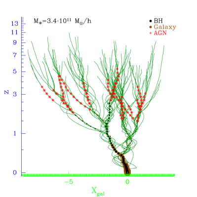
Figure 1: A typical galaxy merger tree in our model. The sizes of brown and black dots are proportional to the stellar mass of the galaxies and to the mass of the central BHs, respectively. The red stars indicate the presence of an AGN and their sizes are proportional to the AGN bolometric luminosities. In the example shown, the merging history of a parent galaxy with stellar mass $M_{\star}=3.4\cdot 10^{11}\,h^{-1}$ ${\rm M}_{\odot}$ is traced back in time from $z=0$, at the bottom of the plot, out to $z\sim 10$. The variable on the horizontal axis represents the displacement between the parent galaxy and its progenitor, defined as $X_{\rm gal}=\sum^{3}_{i=1}(x^{i}_{\rm gal}-x^{i}_{\rm par})$, where $x^{i}_{\rm gal}$ and $x^{i}_{\rm par}$ represent the three Cartesian, comoving components of the progenitor and the parent galaxy, respectively, in unit of $h^{-1}\,\mbox{Mpc}$ .

In order to populate our model galaxies with BHs and AGN, we adopt the following assumptions. The BH mass accretion is triggered by two different phenomena: i) the merger between gas-rich galaxies and ii) the cooling flow at the centres of X-ray emitting atmospheres in galaxy groups and clusters.

The first kind of accretion, dubbed quasar mode, is closely associated with starbursts. Many recent works seem to indicate that major mergers do not constitute the only trigger to BH accretion (see e.g. Marulli et al., 2007; Kauffmann & Heckman, 2008; Hopkins & Hernquist, 2008; Silverman et al., 2008, and reference therein). For this reason, we assume here that any galaxy merger can trigger perturbations to the gas disk and drives gas onto the galaxy centre. BHs can accrete mass both through coalescence with another BH and by accreting cold gas, the latter being the dominant accretion mechanism. The gas mass accreted during a merger is assumed to be proportional to the total cold gas mass of the galaxy (Kauffmann & Haehnelt, 2000), but with an efficiency which is lower for smaller mass systems and for unequal mergers:

$$\Delta M_{\rm BH}=f_{\rm BH}\frac{m_{\rm sat}}{m_{\rm central}}\frac{m_{\rm cold}}{1+V_{\rm vir,280}^{-2}}\,,$$ (1)

where $m_{\rm sat}/m_{\rm central}$ is the total mass ratio of merging galaxies, $m_{\rm cold}$ and $V_{\rm vir,280}$ are the cold gas mass and the virial velocity (in units of $280\,{\rm km\,s^{-1}}$) of the central galaxy, respectively. The parameter $f_{\rm BH}\approx 0.03$ is chosen to reproduce the observed local $M_{\rm BH}-M_{\rm bulge}$ relation (Croton et al., 2006). The accretion driven by major mergers is the dominant mode of BH growth in this scenario. Its energy feedback, which has not been included in the model so far, is approximated by an enhanced effective feedback efficiency for the supernovae associated with the starburst.

Once a static hot halo is formed around a galaxy, we assume that the radio mode sets in, in which a fraction of the hot gas quiescently accretes onto the central BH. During this phase, the accretion rate is typically orders-of-magnitude below the Eddington limit, so that the growth of the BH mass is negligible compared to during the quasar mode phase. However, the energy feedback associated with it injects enough energy into the surrounding medium to reduce or even stop the cooling flow in the halo centres. In this scenario, the effectiveness of radio AGN in suppressing cooling flows is greatest at late times and for large values of the BH mass.

The mass accretion onto the BHs and the associated bolometric luminosity emitted can be described as follows:

$$L_{\rm bol}(t)=f_{\rm Edd}(t)L_{\rm Edd}(t)$$ (2)

$$\frac{d\ln M_{\rm BH}(t)}{dt}={t_{\rm ef}^{-1}(t)}$$ (3)

where $L_{\rm Edd}$ is the Eddington luminosity, $t_{\rm ef}(t)=\frac{\epsilon}{1-\epsilon}\frac{t_{\rm Edd}}{f_{\rm Edd}(t)}$ is the e-folding time ($t_{\rm ef}\equiv t_{\rm Salpeter}$ if $f_{\rm Edd}=1$), $\epsilon$ is the radiative efficiency, $f_{\rm Edd}(t)$ is the Eddington factor and $t_{\rm Edd}=\sigma_{T}c/(4\pi m_{p}G)\sim 0.45\,{\rm Gyr}$. As in M08, we do not follow the evolution of the BH spins and we take a constant mean value for the radiative efficiency of $\epsilon=0.1$ at all redshifts.

We consider three different prescriptions to model $f_{\rm Edd}$, which determines the lightcurves associated with individual quasar events:

• I: $f_{\rm Edd}=1$, the simplest possible assumption.

• II: $f_{\rm Edd}$ is assumed to decrease at low $z$ as suggested by Cattaneo & Bernardi (2003) and Shankar et al. (2004) to match the BH mass function derived from a deconvolution of the AGN luminosity function and the local BH mass function. Here, we adopt the fit derived by Shankar et al. (2004):

  $$f_{\rm Edd}(z)=\left\{\begin{array}[]{ll}0.3&z\geqslant 3\\ 0.3\cdot[(1+z)/4]^{1.4}&z<3\end{array}\right.$$ (4)

• III: the evolution of an active BH is described as a two-stage process of a rapid, Eddington-limited growth up to a peak BH mass, preceded and followed by a much longer quiescent phase with lower Eddington ratios. In this latter phase, the average time spent by AGN per logarithmic luminosity interval can be approximated as (Hopkins et al., 2005)

  $$\frac{{\rm d}t}{{\rm d}\ln L_{\rm bol}}=|\alpha|\,t_{9}\left(\frac{L_{\rm bol}(t)}{10^{9}L_{\odot}}\right)^{\alpha},$$ (5)

  where $t_{9}$ is the total AGN lifetime above $10^{9}L_{\odot}$; $t_{9}\sim 10^{9}\,{\rm yr}$ over the range $10^{9}L_{\odot}<L_{\rm bol}<L_{\rm peak}$, where $L_{\rm peak}$ is the AGN luminosity at the peak of its activity. In the range $10^{10}L_{\odot}\lesssim L_{\rm peak}\lesssim 10^{14}L_{\odot}$, Hopkins et al. (2005) found that $\alpha$ is a function of only $L_{\rm peak}$, given by $\alpha=-0.95+0.32\log(L_{\rm peak}/10^{12}L_{\odot})$, with $\alpha=-0.2$ (the approximate slope of the Eddington-limited case) as an upper limit. Here we interpret the Hopkins model as describing primarily the decline phase of the AGN activity, after the BH has grown at the Eddington rate to a peak mass $M_{\rm BH,peak}=M_{\rm BH}(t_{\rm in})+\mathcal{F}\cdot\Delta M_{\rm BH,Q}\cdot(1-\epsilon)$, where $M_{\rm BH}(t_{\rm in})$ is the initial BH mass and $\Delta M_{\rm BH,Q}$ is the fraction of cold gas mass accreted. We found that $\mathcal{F}=0.7$ is the value that best matches the AGN luminosity function (M08).

  From equation (5) we can derive:

  $$M_{\rm BH}(t)=M_{\rm BH,peak}+\frac{A}{BC}\left[\left(1+Ct\right)^{B}-1\right],$$ (6)

  where $A=\frac{1-\epsilon}{\epsilon}\frac{M_{\rm BH,peak}}{t_{\rm Edd}}$, $B=\frac{1}{\alpha}+1$, $C=\left(\frac{L_{\rm peak}}{10^{9}L_{\odot}}\right)^{-\alpha}\frac{1}{t_{9}}$.

As shown in M08, the semi-analytic models described above underestimate the number density of luminous AGN at high redshifts, independently of the lightcurve model adopted. A significant improvement can be obtained by simply assuming an accretion efficiency that increases with redshift (Croton et al., 2006). In a parallel work, Bonoli et al. (2008), we discuss a model in which the accretion efficiency is linearly dependent on redshift. In the present work however, since our aim is to construct mock catalogues that best reproduce the observed AGN population, we will use the model for the accretion efficiency introduced in M08 to obtain a good match to the AGN luminosity function:

$$\left\{\begin{array}[]{ll}f_{\rm BH}=0.01\cdot\log\left(\frac{M_{\rm BH}}{10^{3}M_{\odot}}+1\right)\cdot z&z>1.5\,{\rm and}\,M_{\rm BH}>10^{6}M_{\odot}\\ {\Delta}M_{\rm BH}=0.01\cdot m_{\rm cold}&z>6\end{array}\right.$$ (7)

Here we keep the prescription III for the quasar lightcurves and, for simplicity, we assume $M_{\rm BH,seed}=10^{3}M_{\odot}$ for all seed BHs, irrespective of their halo host properties and their origin. As in M08, we will refer to this scenario as our best model. Note, however, that future improvements in the underlying physical assumptions may well lead to a yet better model in explaining the observations.

3 Simulating the Chandra deep fields

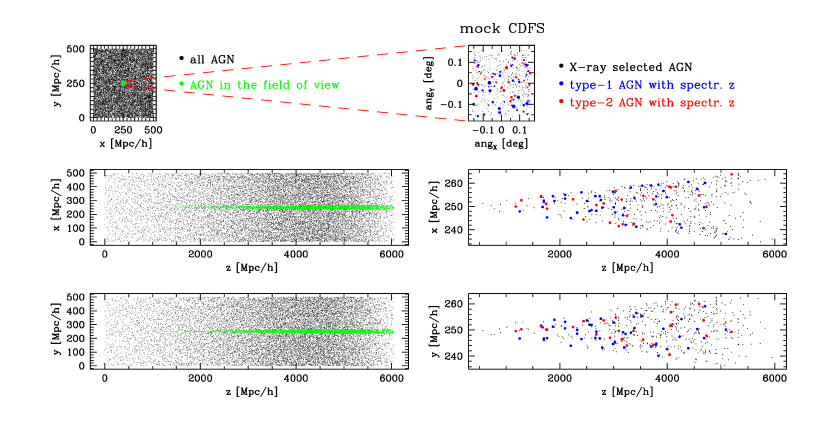
Figure 2: Space-like projections of a past light cone and of a mock field of view with the same selection effects as the CDFS. Left-hand panel: all the AGN predicted by the lightcurve model I (black dots) inside a virtual past light cone and the subpopulation of AGN in a mock CDFS (green dots). Right-hand panel: zoom of the mock field of view represented by the green points in the left panel. The black dots show the AGN that meet the flux-selection criteria. Their number counts and redshift distributions are displayed in Figs. 3 and 4, respectively. The blue and red dots show the type-1 and type-2 AGN in the mock spectroscopic subsample specified in Section 4.2 used to compute the two-point correlation. The size of the red and blue dots in the upper right panel scales as the logarithm of the AGN observed flux.

In order to directly compare our model predictions to the observed number counts and spatial clustering of the X-ray selected AGN in the CDFN and CDFS, we construct a suite of realistic mock AGN catalogues that mimic the selection effects of the real data. The aim is to account for all uncertainties stemming from the conversions between observed and intrinsic AGN properties and to estimate statistical errors. Systematic errors are accounted for by modeling the AGN samples selection effects. Random errors contributed by sparse sampling in the flux limit catalogues and cosmic variance are also taken into account by considering several independent mock samples of AGN with number density comparable to that of the real Chandra fields. Our realistic mock catalogs are obtained by constructing backward light cones from the outputs of the Millennium Simulation . To do this, we have to take into account that redshift varies continuously, whereas the outputs of a simulation have been stored at a finite set of redshifts. To interpolate between discrete redshifts, we have used a technique similar to the standard approach described in the literature (see e.g. Croft et al., 2001; Blaizot et al., 2005; Roncarelli et al., 2006; Kitzbichler & White, 2007), in which the stacking of several computational boxes corresponding to different redshift outputs is performed in comoving coordinates.

To construct mock Chandra fields, we have considered the spatial position and bolometric luminosity of the model AGN in the Millennium Simulation, specified at the available output redshifts, spaced in expansion factor according to $\log(1+z_{n})=n(n+35)/4200$ (Springel et al., 2005). As a first step, we randomly locate a virtual observer in the box at $z=0$ and transform the coordinates to have it at the centre. Then we construct its backward light cone, which extends to $z=5.72$, corresponding to a comoving distance of $\sim 6000$ $h^{-1}\,\mbox{Mpc}$ in our cosmological model, so one would need to stack the simulation volume roughly 12 times. However, we can take advantage of the much denser redshift sampling of the output times (there are $\sim 45$ different outputs between $z=0$ and $z=5.72$) by adopting the following procedure. We divide the light cone into slices along the line of sight based on the output times, so that each slice corresponds to one output and covers the redshift range closest to this output time. To avoid having replicas of the same cosmic structures along the line of sight, we exploit the periodic boundary conditions and adopt the same scrambling technique used by Roncarelli et al. (2006). All CDFs were extracted from different light cones. The procedure is repeated $100$ times, for each of the 4 lightcurve models considered and for the CDFS and CDFN separately (totaling to 400+400 mock CDFs samples). To perform the analysis described in Section 4.2, it is important to estimate how many of theses samples are statistically independent. This can be done by comparing the volume of each sample to that of the Millennium Simulation box, taking into account that the very rare AGN with $z>2$ do not affect the clustering property of the sample and can be safely excluded from the spatial correlation analysis, as we did check. It turns out that, for each lightcurve model, all the 100+100 CDFs extracted from the Millennium box are independent and will be treated as such in the rest of this work. Mock Chandra fields are obtained by mimicking the selection effects of the real samples. To do this, we identify all AGN with the BHs in the quasar phase and discard those too faint to meet the flux-selection criteria. The latter are based on the flux measured in the soft and hard X-ray bands, while our models predict bolometric luminosity. To convert intrinsic bolometric luminosities into soft and hard X-ray bands, we use the bolometric correction proposed by Hopkins et al. (2006), which assumes that the average AGN X-ray spectrum beyond $0.5$ keV can be approximated by a power-law with an intrinsic photon index $\Gamma=1.8$. To transform the intrinsic flux into the observed one, we need to account for photon absorption along the line of sight. To do that, we impose that the intrinsic hydrogen column densities, $N_{\rm H}$, of our AGN are distributed according to La Franca et al. (2005), and that the Galactic $N_{\rm H}$ towards the CDFN and CDFS is $(1.3\pm 0.4)\times 10^{20}\mbox{cm}^{-2}$ and $(8.8\pm 0.4)\times 10^{19}\,\mbox{cm}^{-2}$, respectively. We have checked that using the $N_{\rm H}$ distribution as proposed by Gilli et al. (2007) has a negligible effect on the final results. Only AGN with observed fluxes above the limit $F_{\rm limit}$ of the CDFN and CDFS are included in our mock catalogues. The value of $F_{\rm limit}$ in the CDFN and CDFS varies across the field of view. We account for this effect by adopting the dependency of $F_{\rm limit}$ from the angular distance from the fields’ centre given by Giacconi et al. (2002) and Bauer et al. (2004).

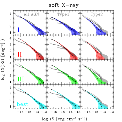
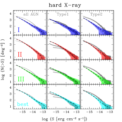
Figure 3: The predicted AGN number counts in the mock CDFs compared to the one determinated by Bauer et al. (2004). The left-hand and right-hand panels display the number counts of the AGN selected in the soft and hard X-ray bands, respectively. The dark and light grey shaded areas show the observed AGN counts obtained with two different classification schemes used to separate AGN from star-forming galaxies. Model predictions: the dashed black curves represents the median of all 100 CDF mocks and the bands indicate the 5th and 95th percentiles. Different colours characterize the different lightcurve models described in Section 2.2, as indicated by the labels.

We have subdivided all mock AGN into type-1 and type-2, according to their $N_{\rm H}$ absorption. AGN with $N_{\rm H}<10^{22}\,\mbox{cm}^{-2}$ are classified as type-1, the more absorbed are classified as type-2. This classification corresponds fairly well to the optical separation into broad-line and narrow-line AGN. All mock CDFN and CDFS pairs are extracted at large angular separation to guarantee independent spatial correlation properties.

The left panels in Fig. 2 show the three space-like projections of a simulated past light cone and of a mock field of view with the same selection effects as the CDFS. The small, black dots represent all model AGN within the cone predicted by the lightcurve model I. The larger, green dots indicate all AGN within a mock CDFS, placed at the centre of the box. The panels on the right zoom in the mock CDFS. In this case, however, the black dots show the AGN that meet the flux-selection criteria specified above. The larger blue and red dots show the type-1 and type-2 AGN in the mock spectroscopic subsample defined in Section 4.2, that will be used to compute the two-point correlation function. The size of the red and blue dots in the upper right panel scales as the logarithm of the AGN observed flux.

4 Model vs. Observations

In this Section, we compare the AGN number counts and spatial clustering predicted by our model with the ones measured in the CDFs. We quantify the dependence of our predictions on the AGN obscuration and on the X-ray selection band. We estimate the effect of the cosmic variance in these deep fields and investigate how robust our conclusions are with respect to the prescription adopted for the AGN lightcurves of individual accretion events. In order to directly compare our predictions to observations, we use the mock AGN catalogues constructed with the technique described in the previous Section.

4.1 AGN number counts

Fig. 3 shows the comparison between the AGN number counts, $N(>S)$, predicted by our model and the ones measured in the CDFs by Bauer et al. (2004), where $N$ is the number of AGN per unit sky area and $S$ is their observed flux. The left-hand and right-hand panels display the number counts of the AGN selected in the soft and hard X-ray band, respectively. The dark and light grey shaded areas show the observed AGN counts obtained with two different classification schemes used to separate AGN from star-forming galaxies, one which conservatively estimates the number of AGN and the other which conservatively estimates the number of star-forming X-ray sources (see Bauer et al., 2004, for details). The dashed black curves represent the median number counts computed over all 100 mock Chandra fields. The surrounding bands indicate the 5th and 95th percentile. Different colours are used to characterize the predictions of the different lightcurve models considered in Section 2.2. As indicated by the labels, the model predictions are separately compared both with the whole AGN population and with the type-1 and type-2 ones. The width of the coloured areas is a measure of the predicted cosmic variance. As shown in Fig. 3, in the flux range covered by the available observed AGN luminosity functions we recover the same results discussed in M08. In particular, if we assume that AGN always shine at the Eddington luminosity (model I, blue), the predicted AGN number density is on average too low in the flux range $\sim 10^{-15}-10^{-14}$ $\mbox{erg}\,\mbox{cm}^{-2}\,\mbox{s}^{-1}$, especially that of the type-2 population. Assuming a lower Eddington ratio at low redshifts, as in our model II (red), or a decline phase of the AGN activity after an Eddington accretion phase up to a peak mass, as in our models III (green) and best (cyan), partly alleviates the problem. However, at $S\lesssim 10^{-15}$ $\mbox{erg}\,\mbox{cm}^{-2}\,\mbox{s}^{-1}$in the soft band, i.e. in a flux range accessible only in the X-ray selected deep fields, our model systematically overestimates the AGN number density, irrespective of the AGN lightcurve model, a mismatch that increases as AGN fluxes and Eddington factor decrease.

To further investigate this point, in Fig. 4 we show the redshift distribution of the AGN in our mock catalogues as a function of the lightcurve model, as indicated by the labels. Each model histogram has been obtained by averaging over 100 mock catalogues. Uncertainties in the model predictions are computed by assuming Poisson statistics. The grey shaded histograms show the redshift distribution measured in the CDFS by Zheng et al. (2004), who used the photometric redshifts of 342 X-ray sources, which constitute $99\%$ of all the detected X-ray sources in the field. The solid black lines show the AGN redshift distributions derived by integrating the bolometric luminosity function of Hopkins et al. (2007). They can be considered as upper limits, since this computation does not account for the sky coverage of the fields, assuming instead a constant flux limit for all the AGN. As can be seen in the Figure, the faint AGN population, overestimated by the model as shown in Fig. 3, is distributed at all redshifts larger than unity. The mismatch is particularly evident in the soft X-ray selected samples.

As we did check, the number density of AGN with fluxes $\gtrsim 10^{-15}$ $\mbox{erg}\,\mbox{cm}^{-2}\,\mbox{s}^{-1}$predicted by all models (apart from model I) is similar to, or slighly smaller than the observed one. On the contrary, all models over-predict the number density of fainter AGN that, however, are typically excluded in the mock CDFs. This discrepancy can be due to one or more of the following reasons: at $S\lesssim 10^{-15}$ $\mbox{erg}\,\mbox{cm}^{-2}\,\mbox{s}^{-1}$, i) the mechanism triggering the BH mass accretion is less efficient than we have assumed, ii) the accretion time is overestimated, iii) the model fraction of obscured AGN is underestimated. Clearly, the model needs to be further developed along these lines to match observations. However, for the purpose of studying the AGN clustering in the CDFs, the over-abundance of faint AGN in our model does not necessairly represent a problem since almost of all of them are excluded from the spectroscopic AGN samples of the CDFs (see below).

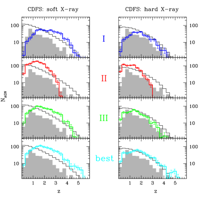
Figure 4: The redshift distribution of the AGN in our mock catalogues (coloured histograms). Uncertainties in the model predictions are computed by assuming Poisson statistics. Grey shaded histograms show the AGN distribution computed in the CDFS by Zheng et al. (2004). The solid black lines display the AGN number counts derived by integrating the bolometric luminosity function of Hopkins et al. (2007).

4.2 AGN spatial clustering

We compare the spatial clustering of AGN in our mock CDFs with those measured in the real catalogues by Gilli et al. (2005) and investigate the dependence on the AGN luminosity. We quantify the AGN clustering properties by means of the two-point auto–correlation function in the real space, $\xi(r)$, using the Landy & Szalay (1993) estimator

$$\xi(r)=\frac{AA(r)-2RA(r)+RR(r)}{RR(r)},$$ (8)

where $AA(r)$, $RA(r)$ and $RR(r)$ are the fraction of mock AGN–AGN, AGN–random and random–random pairs, with spatial separation, $r$, in the range $[r-\delta r/2,r+\delta r/2]$. The random sample is obtained by randomly positioning objects within the same light cones and according to the selection criteria of the AGN sample. The rationale behind computing $\xi(r)$ using spatial positions rather than redshifts is that we wish to compare model predictions with the estimates of Gilli et al. (2005) and Plionis et al. (2008), in which redshift distortions have been corrected for either by projecting the redshift space correlation function or by inverting the measured angular correlation function via Limber’s equation.

To test whether our model is able to match the two-point correlation functions in the CDFs measured by Gilli et al. (2005), we have extracted mock AGN catalogues that closely mimic the spectroscopic AGN samples, in which only objects with good optical spectra, i.e. with spectral quality flag $Q\geq 2$, are considered. For the majority of the AGN in the CDFs, the latter condition is verified when ${\rm M_{R}}<25$, where ${\rm M_{R}}$ is the total apparent magnitude in the R band, i.e. including the contribution of both the AGN and its host galaxy.

To extract a mock spectroscopic subsample, we have computed the R band magnitude of all AGN in the mock Chandra Deep Fields and rejected all objects with ${\rm M_{R}}>25$. In addition, since only about half of the AGN redshifts in the Chandra Deep Fields have been measured, we randomly diluted our sample, keeping only $50\%$ of the mock sources. In Appendix A, we describe the procedure adopted to convert the intrinsic bolometric luminosities of model AGN into apparent R magnitudes, given the redshift of the object and its column density $N_{H}$. The observer frame R magnitudes of the host galaxies have been obtained assuming the parametrization for dust attenuation proposed by De Lucia & Blaizot (2007). We note that the redshift distribution of the mock samples obtained with this procedure is remarkably similar to those observed for the spectroscopic samples of CDFs (e.g. Szokoly et al. 2004, Barger et al. 2003).

The grey shaded areas in the four panels of Fig. 5 represent the power-law model two-point correlation functions that, according to Gilli et al. (2005), best fit the correlation properties of the AGN in the CDFs. We show the case in which the authors fixed the slope to $\gamma=1.4$ in order to focus on the difference in the $r_{0}$ value between the two AGN populations, given the large errors introduced by low number statistics. The latter are modeled as simple Poisson errors. We have repeated the same best fitting procedure to the two-point correlation function measured in each of the mock CDFs. The result is represented by the bands of different colours. Their width represents the field to field variance and accounts for both sparse sampling and cosmic variance. Therefore, these errors quantify the discrepancy between the $r_{0}$ in the data and the models, under the rather strong assumption that $\gamma=1.4$.

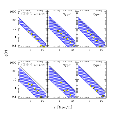
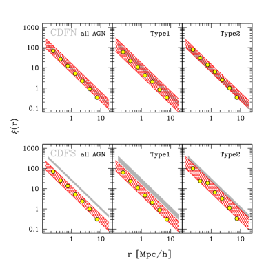
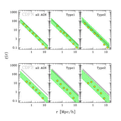
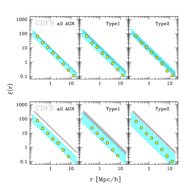
Figure 5: The four panels show the spatial two-point correlation function measured in 100 mock Chandra fields, as a function of the different lightcurve models adopted. The grey shaded areas have been computed using the best-fit power-law model with fixed slope $\gamma=1.4$ adopted by Gilli et al. (2005) to the CDF AGN real space correlation function. As indicated by the labels, the model predictions are compared both with the whole AGN population and with the type-1 and type-2 ones, separately. The yellow dots represent the correlation function of all AGN in the 100 mock Chandra fields. The coloured areas bracket the 5th and 95th percentile of the best-fit power-law to the correlation function in each mock sample (see Table 1). The bandwidth accounts for the different sources of uncertainties, including cosmic variance. The fact that yellow dots are found within the shaded region indicates the adequacy of the best fit model.

		$r_{0}$: CDFN
	all AGN	type 1	type 2
real catalogue	$5.1\,(_{-0.5}^{+0.4})$	$5.6\,(_{-1.0}^{+0.8})$	$4.7\,(_{-1.0}^{+0.8})$
mock I	$3.5\pm 1.7\,(0.8)$	$4.7\pm 4.0\,(1.6)$	$3.7\pm 3.0\,(1.5)$
mock II	$5.4\pm 2.0\,(0.08)$	$5.2\pm 2.6\,(0.2)$	$5.3\pm 1.7\,(0.1)$
mock III	$3.9\pm 1.3\,(0.2)$	$4.3\pm 1.7\,(0.5)$	$5.1\pm 2.1\,(0.4)$
mock best	$4.1\pm 1.3\,(0.2)$	$4.7\pm 1.9\,(0.4)$	$4.8\pm 1.7\,(0.4)$
		$r_{0}$: CDFS
	all AGN	type 1	type 2
real catalogue	$10.4\,(0.8)$	$10.1\,(_{-2.2}^{+1.8})$	$10.7\,(_{-1.6}^{+1.3})$
mock I	$3.7\pm 3.2\,(1.8)$	$5.8\pm 5.0\,(2.7)$	$6.2\pm 4.3\,(2.7)$
mock II	$4.7\pm 1.6\,(0.2)$	$4.9\pm 2.0\,(0.4)$	$6.5\pm 2.9\,(0.4)$
mock III	$4.1\pm 2.0\,(0.6)$	$5.2\pm 3.6\,(1.2)$	$4.8\pm 3.1\,(1.5)$
mock best	$4.2\pm 1.7\,(0.5)$	$5.1\pm 2.6\,(1.0)$	$4.7\pm 3.1\,(1.5)$

Table 1: The best fit parameters: $r_{0}\pm\sigma_{r_{0}}(\langle\rm err(r_{0})\rangle)$, where $\xi(r)=(r/r_{0})^{-1.4}$; $\sigma_{r_{0}}$ are the field-to-field variances of $r_{0}$; $\langle\rm err(r_{0})\rangle$ are the parameters uncertainties averaged over the mock fields.

The yellow dots represent the two-point correlation functions computed using all the AGN pairs in all mock fields. The fact that they are located within the coloured areas indicates the adequacy of the power-law model adopted for the best fit. As in Fig. 3, we show our predictions for the whole AGN population and separately for the type-1 and type-2 AGN.

The parameters of the best fits are listed in Table 1 together with the errors in the form $r_{0}\pm\sigma_{r_{0}}(\langle\rm err(r_{0})\rangle)$, where $r_{0}$ is the best fit value, $\sigma_{r_{0}}$ represents the field-to-field rms and $\langle\rm err(r_{0})\rangle$ is the Poisson uncertainty on $r_{0}$ averaged over all mock fields. When comparing the errors in the mocks, that account for both sparse sampling and cosmic variance, with the Poisson errors of Gilli et al. (2005), we see that the error budget is dominated by cosmic variance. In the CDFN, the correlation length of the mock AGN is consistent with the data. In all models the mean $r_{0}$ value is smaller than the observed one. However, the difference is below 1-$\sigma$. Interestingly, our model predictions for the $r_{0}$ values are in good agreement with the one estimated by considering all extragalactic objects with measured redshifts in the CDFN, including galaxies ($r_{0}=4.2\pm 0.4\,h^{-1}$ Mpc; see Table 2 of Gilli et al., 2005). Since galaxies make up $\sim 30$ % of the spectroscopic sample, this fact could be explained by assuming that most of these galaxies actually contain a weak AGN outshone by their host.

We did also perform a two-parameter fit as in Gilli et al. (2005). In this case, however, the fitting procedure is not robust. Different fitting methods provide different results and the scatter among the best fitting values of $r_{0}$ and $\gamma$ is comparable, and sometimes larger, than their formal error. The effect is larger for model I that predicts significantly less AGN in the CDFs than the other models. Yet, in all models explored a power-law model provides a good fit to the measured $\xi(r)$ which, for the CDFN, is fully consistent with the data. For example, for the model dubbed “best” we have obtained $r_{0}=3.8\pm 0.8$ and $\gamma=1.5\pm 0.3$ in the CDFN and $r_{0}=3.6\pm 0.7$ and $\gamma=1.5\pm 0.4$ in the CDFS, where the quoted errors represent the scatter among the mocks. These values can be compared with the measured values $r_{0}=5.5\pm 0.6$ and $\gamma=1.50\pm 0.12$ in the CDFN and $r_{0}=10.3\pm 1.7$ and $\gamma=1.33\pm 0.14$ in the CDFS. A two parameter fit reduces the differences between the AGN clustering in the CDFN and CDFS. However, the lack of robustness in the two-parameter fitting procedure and the covariance between $r_{0}$ and $\gamma$ hamper a quantitative estimate. We can only conclude that the discrepancy between the model and the observed two-point correlation functions measured in the CDFS is smaller than the 2-2.5 $\sigma$ difference in the correlation lengths $r_{0}$.

Many possible effects may help to further alleviate the tension between model and data. For example, we have seen that the error budget is dominated by cosmic variance that we have estimated using mock catalogs extracted from the Millennium Simulation. Although very large, the computational box is still small for sufficiently rare events. For example, it is not sufficient to contain one $z=6$ Sloan quasar on average. And clustering statistics is more sensitive to simulation volume than most other quantitites one typically considers. Yet, the Millennium Simulation box can accomodate about 100 independent Chandra fields and thus the true variance should not be significantly larger than the estimated one. Alternatively, the analysis of the real data might be affected by errors that have not been accounted for in the analysis of the mock samples. For example, the spatial two-point correlation function of Gilli et al. (2005) has been obtained from the projected one assuming a power-law model. Possible deviations from the power-law shape would also contribute to errors. However, according to our models, these errors should be negligible, since the mock AGN correlation function is well approximated by a power law. Several examples can be worked out. However, in order to significantly affect our results, these hidden errors must be comparable to cosmic variance which, as we have seen, is larger than sparse sampling error.

Uncertainties in model predictions provide an additional way to reduce the discrepancy between model and data. For example, the clustering of our mock AGN could be enhanced by forcing models to preferentially populate highly biased, massive haloes. This would increase the AGN correlation length in both CDFN and CDFS and reduce the mismatch between model and data. More physically motivated AGN models may predict very different properties for AGN that populate haloes of a given mass. This would increase the so-called stochasticity of the AGN bias and increase the size of the coloured regions in Fig. 5 (Dekel & Lahav, 1999; Sigad et al., 2000). However, it is not at all obvious how to achieve this task.

The other possibility, of course, is that the discrepancy between CDFN and CDFS is significant and that the observed clustering of the AGN in the CDFS is unusually large. An indication that this may indeed be the case is provided by the AGN two-point correlation function recently measured in the XMM-COSMOS fields by Gilli et al. (2009) which is consistent with that of CDFN and, as we have verified, with our model predictions, but not with that of CDFS.

Finally, as can be seen in Fig. 5, we stress that our conclusions are robust with respect to the lightcurve model assumed. Moreover, as we have verified, our results are almost unchanged when using different assumptions in converting AGN bolometric luminosities into optical apparent magnitudes.

4.2.1 Luminosity dependent AGN clustering

Plionis et al. (2008) have recently investigated the clustering of the AGN in the CDFs as a function of their luminosity. The authors have measured the two-point angular correlation function of the objects in different flux-limited subsamples and then used Limber’s equation to derive the spatial clustering length $r_{0}$. They found a strong dependence of $r_{0}$ on the median X-ray luminosity of each flux-limited subsample in both the CDFN and CDFS and in the soft and hard X-ray band.

To investigate whether we find a similar trend in our model, we have extracted different flux-limited subsamples from the mock Chandra fields, characterized by different values of $F_{\rm limit}$ and, therefore, by a median X-ray luminosity $\langle L_{\rm AGN,X}\rangle$. The clustering length of the mock AGN in each subsample has been estimated by fitting their spatial two-point correlation functions with a power-law. The results are shown in Figure 6, in which we plot the values of $r_{0}$ as a function of $\langle L_{\rm AGN,X}\rangle$ for the AGN in the mock CDFN (upper panels) and CDFS (bottom panels). The results of our four lightcurve models are represented by different symbols (model I: blue triangles, II: red squares, III: green pentagons, best: cyan hexagons) and compared with the results of Plionis et al. (2008) (black dots). Model predictions have been obtained by averaging over $100$ different mock catalogues for each lightcurve model. Errors show the scatter among the mock fields.

In all models the correlation length is almost constant with luminosity, showing just a slight increase at high luminosities, in disagreement with the strong luminosity dependence $r_{0}$ found by Plionis et al. (2008). Although small, the precise trend in the mock catalogues depends on the lightcurve model adopted. For instance, in model best the dependence is quite mild, while in model II $r_{0}$ significantly increases already above $\langle L_{\rm AGN,X}\rangle\sim 10^{42.5}\mbox{erg}\,\mbox{s}^{-1}$. The spread in the model predictions makes the clustering luminosity dependence a possible observational test to discriminate among different theoretical models if they can be compared with larger samples in order to reduce the size of the error bars. The sample of AGN with measured redshift in the 2 deg² XMM-COSMOS field represents an important step in this direction. Interestingly enough, the correlation length of $\sim 500$ AGN with typical X-ray luminosity of $10^{43.8}\mbox{erg}\,\mbox{s}^{-1}$ in the 0.5-10 keV band is in the range 6-8 $h^{-1}\,\mbox{Mpc}$ (depending on whether a prominent structure at $z=0.36$ is included or not in the sample), significantly smaller than the value estimated by Plionis et al. (2008) and in good agreement with the one predicted by our models (Gilli et al. 2008).

We note that a global study of the clustering properties of simulated AGN not restricted to the Chandra fields will be presented in Bonoli et al. (2008). We anticipate here a similar result for the luminosity dependence of AGN clustering: $r_{0}$ is found to be only weakly dependent on luminosity, in particular in the redshift range $z\sim 2-3$, that corresponds to the peak of the AGN number density.

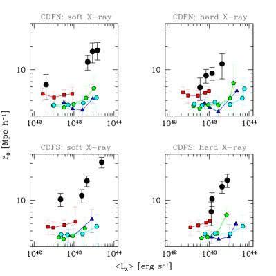
Figure 6: The values of $r_{0}$ as a function of the median X-ray luminosity $\langle L_{\rm AGN,X}\rangle$ for the AGN in the mock CDFN (upper panels) and CDFS (bottom panels). The results of our four lightcurve models are represented by different symbols (I: blue triangles, II: red squares, III: green pentagons, best: cyan hexagons) and compared with the results of Plionis et al. (2008) (black dots). Model predictions have been obtained by averaging over $100$ different mock catalogues for each lightcurve model. Errors show the scatter among the mock fields.

5 Conclusions

In this paper, we modelled the AGN spatial distribution measured in the Chandra deep fields within the framework of hierarchical co-evolution of BHs and their host galaxies. For this purpose, we have applied the semi-analytic techniques developed by Croton et al. (2006), De Lucia & Blaizot (2007) and M08 to follow the cosmological evolution of AGN inside the Millennium Simulation (Springel et al., 2005), and extracted a number of independent mock catalogues of AGN that closely resemble the CDFS and CDFN. Each mock CDF catalogue has been obtained by including all AGN within a past light cone of a generic observer that meet the same selection criteria (field of view, flux limit, edge effects) as the real sample. The large volume of the Millennium Run allowed us to extract hundreds of independent mock CDFs in which we have measured the spatial two-point correlation function of the mock AGN in real-space. We have ignored redshift space distortions since these are already corrected for in the observational estimates of Gilli et al. (2005) and Plionis et al. (2008), which we wish to compare with.

The main results of this study can be summarized as follows:

(i) The number counts of bright model AGN agree with observations both in the soft and in the hard X-ray bands. The abundance of model AGN at fluxes below $\lesssim 10^{-15}$ $\mbox{erg}\,\mbox{cm}^{-2}\,\mbox{s}^{-1}$, however, is larger than observed. The amplitude of the mismatch depends on the lightcurve model explored and on the AGN intrinsic absorption. In fact, our models seem to underpredict the abundance of type-2 objects.

(ii) The number of mock AGN in the simulated CDFs in the redshift range $1.5\lesssim z\lesssim 4$ is higher than observed in the soft X-ray band. The mismatch is less evident in the hard X-ray band. This discrepancy in the redshift distributions is not unexpected since, as discussed by M08, the same hybrid model considered in this work over-predicts the abundance of faint objects with redshift in the range $z\lesssim 4$ (see their Fig.7).

(iii) The spatial two-point correlation function predicted by all lightcurve models is well described by a power-law out to 20 $h^{-1}\,\mbox{Mpc}$ . If one set the slope $\gamma=1.4$, as in Gilli et al. (2005), then the correlation length $r_{0}$ agrees, to within 1 $\sigma$, with that measured by Gilli et al. (2005) in the CDFN once cosmic variance is accounted for. On the contrary, the mock AGN in the CDFS are much less correlated than the real one. In this case, the discrepancy in the correlation lenght is of the order of 2-2.5 $\sigma$, depending on the lightcurve model adopted.

(iv) The mismatch is alleviated by performing a two-parameter fit to the two-point correlation function. However, a quantitative estimate is hampered by the lack of robustness in the two-parameter fitting procedure which results from low number statistics. The tension between model and data is further alleviated by possible observational errors that are not properly accounted for and by model uncertainties. Overall, one expects that the discrepancy between the observed and modeled $\xi(r)$ is smaller than the 2-2.5 $\sigma$ mismatch in the correlation lengths quoted previously.

(v) The agreement between correlation functions in the XMM-COSMOS field (Gilli et al., 2009) and in the CDFN which, as we have shown, is well reproduced by our AGN models suggests that the AGN clustering in the CDFS is indeed unusually high.

(vi) The models predict that the clustering amplitude depends little on the luminosity of AGN, in disagreement with the strong dependence found by Plionis et al. (2008) but in agreement with the measurements of the clustering of luminous AGN in the recently complied XMM-COSMOS catalogue (Gilli et al., 2009).

Precise predictions for the luminosity dependence of the AGN clustering depend on the adopted theoretical models, and their present mutual agreement merely reflects the still large field-to-field variance. Therefore, one can hope that measuring the AGN clustering properties as a function of their luminosity in larger datasets could help discriminating among the models. Furthermore, going beyond the spatial AGN autocorrelation function, the analysis of the cross-correlation between AGN and galaxies in the next generation all-sky surveys at $z\geq 1$, like EUCLID or ADEPT, will place strong constraints on modern semi-analytic models, thereby shedding light on the complicated mechanisms that regulate the co-evolution of AGN and galaxies.

Appendix A From AGN intrinsic luminosities to observed magnitudes

To convert the intrinsic bolometric luminosities of the model AGN, $L_{\rm bol}$, into absorbed apparent R-band magnitudes, given the AGN redshift and $N_{\rm H}$, we make the following steps. First, we use the bolometric correction given by Hopkins et al. (2006) to get the AGN intrinsic B-band luminosity, $L_{\rm B}$. Then, we get the monochromatic unabsorbed R-band luminosity, assuming:

$$L^{\rm UNABS}_{\nu}=L_{B,\nu}\left(\frac{\nu}{\nu_{B}}\right)^{-0.44}\,,$$ (9)

where

$$L_{B,\nu}=\frac{\lambda^{2}}{c}L_{B,\lambda}\sim\frac{\lambda^{2}}{c}\frac{L_{B}}{\Delta\lambda_{B}}\,,$$

$\nu_{B}=c/(445\rm nm)$, $\nu=(1+z)\nu_{R}=(1+z)c/(658\rm nm)$, $\Delta\lambda_{B}\sim 100\rm nm$ and $c$ is the speed of light. The absorbed monochromatic luminosity can be obtained with the following equation:

$$L^{\rm ABS}_{\nu}=L^{\rm UNABS}_{\nu}\times 10^{-0.4\,A}\,,$$ (10)

where

$$A=A_{V}\left(1+\frac{1}{3.1}(0.000843x^{5}-0.02496x^{4}+\right.\\ \left.0.2919x^{3}-1.815x^{2}+6.83x-7.92)\right)\,,$$ (11)

$x=\lambda^{-1}$ in $\mu m^{-1}$ and $A_{V}=5\times 10^{-22}N_{\rm H}$ (Gaskell & Benker, 2007).

Finally, to get the apparent R magnitude in the observer frame, we use:

$$R_{\rm AB}=8.9-2.5\log(f_{\nu}/Jy)\,,$$ (12)

where $f_{\nu}$, the monochromatic flux expressed in units of Jansky, is:

$$f_{\nu}=(1+z)\frac{L^{\rm ABS}_{\nu}}{4\pi d_{L}(z)^{2}}\,,$$ (13)

and $d_{L}(z)$ is the luminosity distance.

To get the total R-band magnitudes of mock objects, the AGN magnitude computed as described above is finally combined with that of the host galaxies obtained by De Lucia & Blaizot (2007).

References

- Alexander et al. (2003) Alexander D. M., et al., 2003, AJ, 126, 539
- Barger et al. (2003) Barger A. J., et al., 2003, AJ, 126, 632
- Bauer et al. (2004) Bauer F. E., Alexander D. M., Brandt W. N., Schneider D. P., Treister E., Hornschemeier A. E., Garmire G. P., 2004, AJ, 128, 2048
- Binney & Tremaine (1987) Binney J., Tremaine S., 1987, Galactic dynamics. Princeton, NJ, Princeton University Press, 1987, 747 p.
- Blaizot et al. (2005) Blaizot J., Wadadekar Y., Guiderdoni B., Colombi S. T., Bertin E., Bouchet F. R., Devriendt J. E. G., Hatton S., 2005, MNRAS, 360, 159
- Bonoli et al. (2008) Bonoli S., Marulli F., Springel V., White S. D. M., Branchini E., Moscardini L., 2008, ArXiv e-prints
- Cattaneo & Bernardi (2003) Cattaneo A., Bernardi M., 2003, MNRAS, 344, 45
- Cattaneo et al. (2005) Cattaneo A., Blaizot J., Devriendt J., Guiderdoni B., 2005, MNRAS, 364, 407
- Colless et al. (2001) Colless M., et al., 2001, MNRAS, 328, 1039
- Croft et al. (2001) Croft R. A. C., Di Matteo T., Davé R., Hernquist L., Katz N., Fardal M. A., Weinberg D. H., 2001, ApJ, 557, 67
- Croom et al. (2005) Croom S. M., et al., 2005, MNRAS, 356, 415
- Croton et al. (2006) Croton D. J., et al., 2006, MNRAS, 365, 11
- Croton & Farrar (2008) Croton D. J., Farrar G. R., 2008, ArXiv e-prints, 801
- De Lucia & Blaizot (2007) De Lucia G., Blaizot J., 2007, MNRAS, 375, 2
- De Lucia & Helmi (2008) De Lucia G., Helmi A., 2008, ArXiv e-prints, 804
- De Lucia et al. (2004) De Lucia G., Kauffmann G., Springel V., White S. D. M., Lanzoni B., Stoehr F., Tormen G., Yoshida N., 2004, MNRAS, 348, 333
- De Lucia et al. (2004) De Lucia G., Kauffmann G., White S. D. M., 2004, MNRAS, 349, 1101
- De Lucia et al. (2006) De Lucia G., Springel V., White S. D. M., Croton D., Kauffmann G., 2006, MNRAS, 366, 499
- Dekel & Lahav (1999) Dekel A., Lahav O., 1999, ApJ, 520, 24
- Di Matteo et al. (2008) Di Matteo T., Colberg J., Springel V., Hernquist L., Sijacki D., 2008, ApJ, 676, 33
- Efstathiou (1992) Efstathiou G., 1992, MNRAS, 256, 43P
- Elbaz et al. (2007) Elbaz D., et al., 2007, A&A, 468, 33
- Ferrarese & Ford (2005) Ferrarese L., Ford H., 2005, Space Science Reviews, 116, 523
- Fontanot et al. (2006) Fontanot F., Monaco P., Cristiani S., Tozzi P., 2006, MNRAS, 373, 1173
- Gaskell & Benker (2007) Gaskell C. M., Benker A. J., 2007, ArXiv e-prints, 711
- Giacconi et al. (2002) Giacconi R., et al., 2002, ApJS, 139, 369
- Gilli et al. (2007) Gilli R., Comastri A., Hasinger G., 2007, A&A, 463, 79
- Gilli et al. (2005) Gilli R., et al., 2005, A&A, 430, 811
- Gilli et al. (2007) Gilli R., et al., 2007, A&A, 475, 83
- Gilli et al. (2009) Gilli R., et al., 2009, A&A, 494, 33
- Graham (2008) Graham A. W., 2008, ApJ, 680, 143
- Grazian et al. (2004) Grazian A., Negrello M., Moscardini L., Cristiani S., Haehnelt M. G., Matarrese S., Omizzolo A., Vanzella E., 2004, AJ, 127, 592
- Hopkins & Hernquist (2008) Hopkins P. F., Hernquist L., 2008, ArXiv e-prints
- Hopkins et al. (2008) Hopkins P. F., Hernquist L., Cox T. J., Kereš D., 2008, ApJS, 175, 356
- Hopkins et al. (2006) Hopkins P. F., Hernquist L., Cox T. J., Robertson B., Di Matteo T., Springel V., 2006, ApJ, 639, 700
- Hopkins et al. (2005) Hopkins P. F., Hernquist L., Martini P., Cox T. J., Robertson B., Di Matteo T., Springel V., 2005, ApJ, 625, L71
- Hopkins et al. (2007) Hopkins P. F., Richards G. T., Hernquist L., 2007, ApJ, 654, 731
- Kauffmann & Haehnelt (2000) Kauffmann G., Haehnelt M., 2000, MNRAS, 311, 576
- Kauffmann & Heckman (2008) Kauffmann G., Heckman T. M., 2008, ArXiv e-prints
- Kitzbichler & White (2007) Kitzbichler M. G., White S. D. M., 2007, MNRAS, 376, 2
- La Franca et al. (2005) La Franca F., et al., 2005, ApJ, 635, 864
- Landy & Szalay (1993) Landy S. D., Szalay A. S., 1993, ApJ, 412, 64
- Lemson & Virgo Consortium (2006) Lemson G., Virgo Consortium t., 2006, preprint, astro-ph/060801
- Li et al. (2007) Li Y., Hernquist L., Robertson B., Cox T. J., Hopkins P. F., Springel V., Gao L., Di Matteo T., Zentner A. R., Jenkins A., Yoshida N., 2007, ApJ, 665, 187
- Luo et al. (2008) Luo B., et al., 2008, ArXiv e-prints, 806
- Magorrian et al. (1998) Magorrian J., et al., 1998, AJ, 115, 2285
- Malbon et al. (2007) Malbon R. K., Baugh C. M., Frenk C. S., Lacey C. G., 2007, MNRAS, 382, 1394
- Marconi & Hunt (2003) Marconi A., Hunt L. K., 2003, ApJ, 589, L21
- Marulli et al. (2008) Marulli F., Bonoli S., Branchini E., Moscardini L., Springel V., 2008, MNRAS, 385, 1846
- Marulli et al. (2007) Marulli F., Branchini E., Moscardini L., Volonteri M., 2007, MNRAS, 375, 649
- Marulli et al. (2006) Marulli F., Crociani D., Volonteri M., Branchini E., Moscardini L., 2006, MNRAS, 368, 1269
- Mateus (2008) Mateus A., 2008, ArXiv e-prints, 802
- McCracken et al. (2007) McCracken H. J., et al., 2007, ApJS, 172, 314
- Mo et al. (1998) Mo H. J., Mao S., White S. D. M., 1998, MNRAS, 295, 319
- Pelupessy et al. (2007) Pelupessy F. I., Di Matteo T., Ciardi B., 2007, ApJ, 665, 107
- Plionis et al. (2008) Plionis M., Rovilos M., Basilakos S., Georgantopoulos I., Bauer F., 2008, ApJ, 674, L5
- Porciani et al. (2004) Porciani C., Magliocchetti M., Norberg P., 2004, MNRAS, 355, 1010
- Porciani & Norberg (2006) Porciani C., Norberg P., 2006, MNRAS, 371, 1824, [PN06]
- Roncarelli et al. (2006) Roncarelli M., Moscardini L., Tozzi P., Borgani S., Cheng L. M., Diaferio A., Dolag K., Murante G., 2006, MNRAS, 368, 74
- Rosati et al. (2002) Rosati P., et al., 2002, ApJ, 566, 667
- Sánchez et al. (2006) Sánchez A. G., Baugh C. M., Percival W. J., Peacock J. A., Padilla N. D., Cole S., Frenk C. S., Norberg P., 2006, MNRAS, 366, 189
- Shankar et al. (2004) Shankar F., Salucci P., Granato G. L., De Zotti G., Danese L., 2004, MNRAS, 354, 1020
- Sigad et al. (2000) Sigad Y., Branchini E., Dekel A., 2000, ApJ, 540, 62
- Sijacki et al. (2007) Sijacki D., Springel V., di Matteo T., Hernquist L., 2007, MNRAS, 380, 877
- Silverman et al. (2008) Silverman J. D., et al., 2008, ArXiv e-prints
- Somerville et al. (2001) Somerville R. S., Primack J. R., Faber S. M., 2001, MNRAS, 320, 504
- Spergel et al. (2003) Spergel D. N., et al., 2003, ApJS, 148, 175
- Springel et al. (2005) Springel V., et al., 2005, Nat, 435, 629
- Springel et al. (2001) Springel V., White S. D. M., Tormen G., Kauffmann G., 2001, MNRAS, 328, 726
- Tremaine et al. (2002) Tremaine S., et al., 2002, ApJ, 574, 740
- Volonteri et al. (2003) Volonteri M., Haardt F., Madau P., 2003, ApJ, 582, 559
- Wang et al. (2007) Wang J., De Lucia G., Kitzbichler M. G., White S. D. M., 2007, preprint, astro-ph/0706.2551, 706
- Weinmann et al. (2006) Weinmann S. M., van den Bosch F. C., Yang X., Mo H. J., Croton D. J., Moore B., 2006, MNRAS, 372, 1161
- White & Frenk (1991) White S. D. M., Frenk C. S., 1991, ApJ, 379, 52
- Zheng et al. (2004) Zheng W., et al., 2004, ApJS, 155, 73